Reproducibility of the Quantification of Reversible Wall Interactions in VOC Sampling Lines

Abstract

Volatile Organic Compounds (VOCs) are widely measured at ppb and ppt level in many contexts, from therapeutic drug control in respiratory diseases to monitoring of climate change and indoor air quality. The need for accuracy is a common denominator in all these fields. The interactions between gas mixtures and solid surfaces in sampling lines and instruments play an important role in calculating the total uncertainty of the amount of VOC. The amount of substances in the gas mixture is affected by its reversible and irreversible interactions with the sampling line. The main aim of this paper is to propose and discuss a method to quantify the amount of substance segregated by reversible interactions on sampling lines. To validate the proposed method, the areic amount of a VOC (Acetone) is measured for a commercial test pipe (Sulfinert^®) as the amount of substance per unit area of the internal surface of the test pipe segregated from the flowing gas mixture. Stainless steel coated by Sulfinert^® was chosen as a test material because of its wide use and its limited irreversible and permeation effects. A certified gas mixture of Acetone in air with a nominal mole fraction of 10 µmol mol⁻¹ was used for validation. Broad temperature control was used and the sensibility of the method to the temperature and the pressure has been evaluated to correct the bias due to physical condition. The sensitivity to the residence time and the Reynolds number of the gas flow has been evaluated to verify the reaching of equilibrium and the limits of the applicability of the method. The areic amount of Acetone at equilibrium on Sulfinert^® coated pipe was measured as 40 nmol m⁻², and an equilibrium constant value of around 0.2 m was calculated as the ratio between the superficial amount segregated on the wall and the amount concentration of Acetone in the mixture, both at the equilibrium. The observed reproducibility was better than 2.5%. This method is aimed to investigate VOC losses due to interactions for many VOC/material systems at a lower amount of substance levels.

1. Introduction

The measurements of volatile organic compounds (VOCs) at trace level have a major role in atmospheric chemistry, health, ultra-clean industrial processes, indoor air quality, and metrology [1,2]. In all these applications, measurements of VOCs amount of substance require a challenging target accuracy at the level of pmol mol⁻¹ (ppt) and nmol mol⁻¹ (ppb) [1]. VOCs’ monitoring within 1–1000 ppb range is required for the atmosphere and indoor air quality at an uncertainty of 5% for different VOCs and 3% for different fluorinate volatile compounds [3,4,5]. VOCs are ozone precursors that affect ozone production in the presence of NOx and light; these are harmful pollutants at a lower altitude [6]. VOCs having C=C double bonds are more reactive, which upon oxidation produces a large variety of particle-phase compounds that are more hazardous than the original one [7]. Indoor VOC concentrations are higher than outdoor ones [8,9], and human exposure to these VOCs can have short- and long-term adverse effects on their health. Many VOCs are also considered to be Airborne Molecular Contaminants (AMCs), which can be a threat to the yield of ultra-sensitive manufacturing processes such as semiconductor, nanotechnology, and photovoltaics that raises the need for accuracy in measurements at ppb level [10,11,12]. A good estimation of uncertainty in measurements of emitted VOCs from different parts of the human body is essential due to its role as a biomarker that is used to detect different diseases including lung cancer [13,14,15,16,17].

VOCs monitoring, regardless of the application, requires the use of pipes, fittings, liners, cylinders, joints, pressure regulators, environmental chambers, generation devices, and measurement instruments, all built using solid materials of different nature. In all these applications, the gas–wall interactions affect the mole fraction of VOCs [18,19,20,21,22,23,24,25,26]. Sampling pipes that convey the air from the atmosphere to the detectors can potentially disturb the measurement of the amount of the analyte segregating on or releasing from the wall surfaces, i.e., these interactions challenge the accuracy of the measurement [26]. The gas mixtures interact by adsorption, desorption, and reactions with the available surfaces, both at the wall or, by permeation, inside of it [27].

The adsorption and desorption of gases over the surfaces are the sum of collective phenomena that occur in series and/or parallel [28]. The gas–wall interactions cause reversible and irreversible losses that depend on the different parameters such as contact time, contact area, and thermodynamic conditions [29]. The characteristics of the analyte, e.g., polarities and molecular mass, are crucial in determining the nature and intensity of interactions [30]. Losses due to interactions are significant for oxygenated VOCs (Oxy-VOCs) and Terpenes because of their high affinity with the wall that leads to adsorption and reactions [5,30,31]. The lower the Oxy-VOC mole fraction is the more important it is to use suitable materials to minimize losses on wall surfaces.

Interactions with polymeric materials like PFA (Perfluoroalkoxy alkanes) and FEP (fluorinated ethylene propylene) are very small; polymeric materials are recommended for sampling lines [26,32,33,34]. However, polymers can cause undesirable effects because of their permeability for gases while glass and metals because of their affinity for surface adsorption and reactions [30,35].

Where reaction products are formed by gas to wall interactions, identification of substances can be difficult [36]. Interactions can affect the stability and accuracy of the standard gas mixture at trace level for both static and dynamic preparations [5,18,19,31,37,38,39]. The losses due to interactions in cylinders had been widely investigated in References [40,41,42,43,44,45,46]. A method for the estimation of losses in cylinders has recently been proposed [37].

The impact of the gas–wall interactions on VOCs’ measurements in sampling lines has been recently under study [1,5,20,22,31,47,48,49,50], but results are still limited. Teflon, polymeric material, coated and uncoated steel, glass, and aluminum have been considered. A comparison of interactions of gas mixtures and different materials was based on the absorptive partitioning effects on delays; Teflon and PFA proved to be the best at a level of 100 μg m⁻³ [20,48]. Quantification of gas–wall partitioning was proposed on Teflon chambers [22]. Chambers has a reduced control of local fluid dynamic conditions and subjected to buoyancy effects [22].

Quantification of losses aimed to correct a bias in VOC measurement has not yet been proposed, to this aim, a correction has to be quantified with a proper target accuracy. Simplified conservative quantification of the losses due to gas–wall interactions in the sampling lines has been proposed, it is based on the value of an equilibrium amount of VOC adsorbed on the pipe wall [1]. A quantification of equilibrium amount segregated on the material surface is available from theoretical insight and models for few types of wall materials [30]. Equilibrium between gas mixtures and pipe walls is expected to be at a constant ratio between potentials on the two phases expressed as an amount per unit volume of mixture and amount per unit active surface of pipe wall [30]. Experimental methods have been proposed in research projects [5,31], the preliminary results showed a very large uncertainty in theoretical previsions and a low reproducibility in experimental data [31]. The purpose is to investigate interaction at a very low level using a PTR-MS as detectors [5], but the risk of working at a low level is to have instability of sources that do not allow to have reliable data on the material properties. This paper is aimed to fix a starting point of a quantitative method for the measure of reversible interactions before applying the method to a low amount of substance.

The novelty of the paper is the proposal of a quantitative method for reproducible measurement of interactions in sampling lines to offer reliable data to calculate the biases affecting VOC measurements. This paper describes the method in detail and discusses the reproducibility of an application to measure the reversible interactions between a VOC (Acetone) gas mixture and a commercial pipe, which is typically used for sampling when interactions can be critical (Sulfinert^®). An experimental set-up has been designed, in which a mixture containing a single VOC was flushed inside a clean test pipe. A fast response detector was used to retrieve the signal of VOC concentration. The amount of VOC segregated from the mixture was calculated from the depletion of the signal. The amount of VOC segregated per unit area (C_A,e) was considered to calculate an equilibrium constant (K_e) of VOC adsorption on the internal surface of the test pipe. The acetone (CH₃-CO-CH₃) mixture in air at the ppm level with certified uncertainty is used for the experiments due to the stability of acetone, its high response on the detector, and its importance in applications [3,5,31,51]. The chosen test material was Sulfinert^® because the stainless steel pipe wall limits the permeation rate and the silicon inert coating limits gas–wall interactions, the irreversible ones in particular. Materials and operating conditions were selected to limit the risk of instability and low reproducibility due to the source of mixtures, to the detection system, and to the mutual effects of other interaction ways (irreversible interactions and permeation).

The correction of biases in measurements was discussed. The paper reports sensitivities of the areic adsorbed amount to the contact time between gas mixture and pipe, and to the fluid dynamic conditions. The sensitivity tests were performed on a wide range of gas flow rates and with different lengths of test pipe in order to verify if transport phenomena are affecting the measurement.

2. Materials and Methods

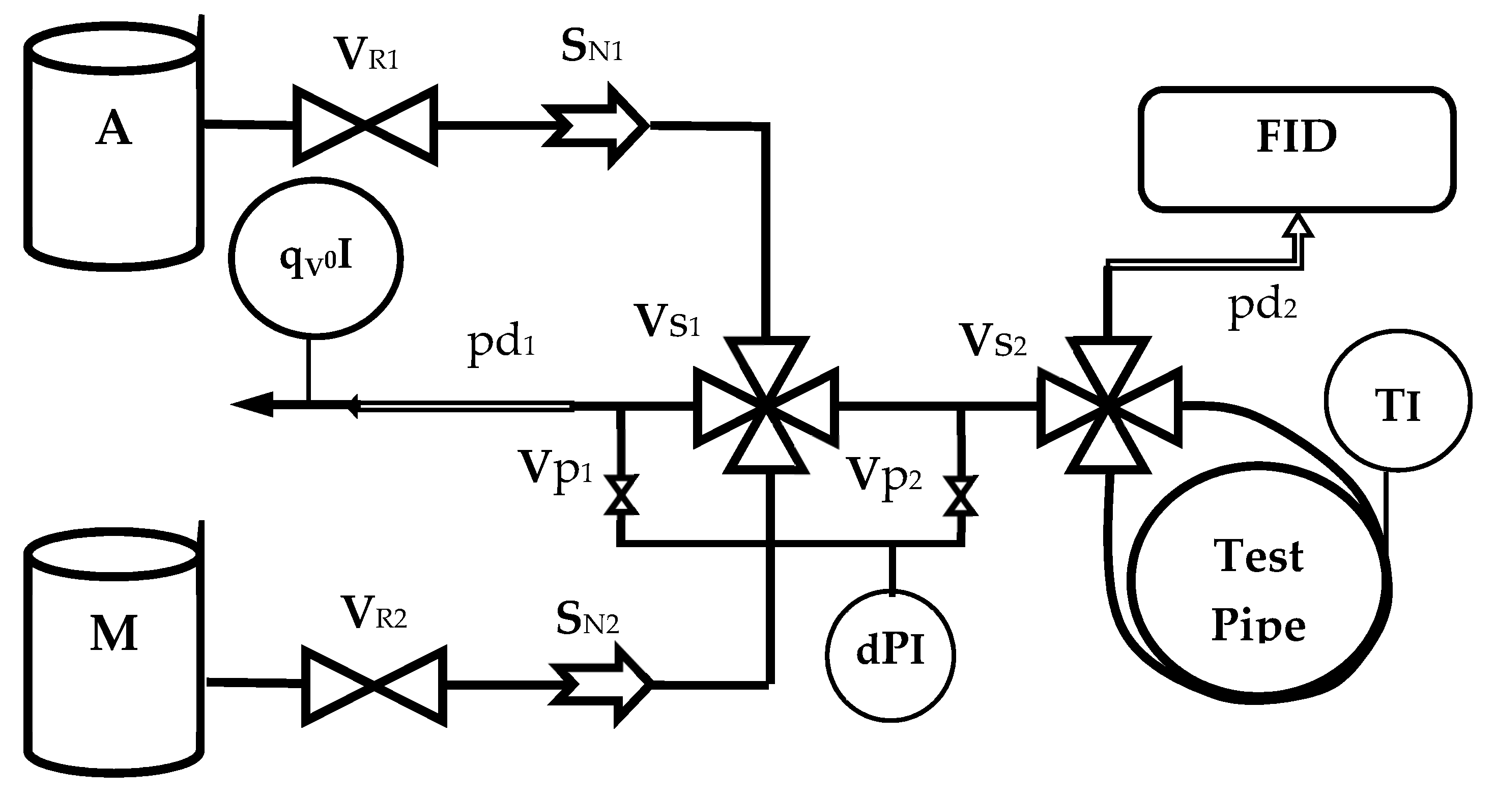
2.1. Experimental Set-Up

An experimental set-up for the quantification of the gas–wall interaction has been developed. The set-up allows to switch the feed to a detector between two different sources of gas, i.e., Zero gas (VOC free) or VOC Mixture, directly or through a test pipe. The schematic drawing is shown in Figure 1. The Zero gas obtained from a commercial dry air cylinder (A) is considered with a negligible amount of hydrocarbons. The VOC Mixture source is a cylinder containing a certified reference mixture of Acetone in air (M). Each feed has a controlled flowrate, sources A and M are connected to sonic nozzles (S_N1 and S_N2) and regulated by the pressure-reducing valves (V_R1 and V_R2) to deliver a stable flowrate for each experiment. Two identical 4-way crossover valves with a limited contact surface and dead volume have been chosen to select between feeds A and M (V_s1) and between bypass and test pipe (V_s2). The valve V_s1 switches the feed A or M stream between a vent line to measure the mass flow rate (q_V0I) and a detector line (flame ionization detector (FID)). The valve V_s2 has 2 identical internal ducts, one of them acts as a bypass, the second one is accounted as a part of the test pipe. The Flame ionization detector (FID) of a gas chromatograph (Bruker GC-450) is used for the detection of VOC in the feed after the test pipe/bypass. The mass flow rate is measured by two 100 SmL/min Bronkhorst mass flow meters (q_V0I) operating in parallel to reach a total full scale of 200 SmL/min. The test pipes have been insulated by polystyrene sheets to improve temperature stability. Test runs with different setpoints for the room temperature have been performed, in the range from 17 °C to 30 °C.

Time variability of ±2 °C and spatial variability of ±2 °C have been observed in the test pipe external wall. The temperature of the test pipe is measured with calibrated temperature sensors Pt-100 (TI) on the external surface of the test pipe during the experiments in different positions along the test pipe.

Pressure spikes occur when V_s1 is switched, they are limited by keeping the same pressure drop on the vent and the FID line by additional pressure drops in capillary pipes pd₁ and pd₂. The pressure drop was measured by a Yokogawa MT-110 (dPI) as the differential pressure from the room atmospheric pressure. Valves V_p1 and V_p2 allow measuring the pressure drop on the vent line and the FID line, respectively.

The system is checked periodically for leaks using the procedure described in Reference [1]. Leak tests are performed after FID signal stabilization at the initial switch-on (at least two hours). The residence time of the gas stream in the test pipe (τ_r, min) is estimated as the ratio between the internal test pipe volume (V_t, mL) and the gas volumetric flow rate (q_V,g, mL min⁻¹):

$${\tau }_r=\frac{V_t}{q_{V,g}}=\frac{\frac{\pi D^{2}L}{4}}{q_{V^0,g}\frac{P^0}{P} \frac{T}{T^0}}$$

(1)

where D (cm) and L (cm) are the internal diameter and length of the test pipe, respectively; T (K) and P (kPa) are average temperature and pressure in the test pipe, respectively; dP (kPa) is the pressure drop on FID line; superscript 0 accounts for standard condition (0 °C, 1 bar); q_V0,g (SmL min⁻¹) is the mass flow rate expressed as volumetric flow rate at standard condition measured by the mass flow meter. The average pressure in the pipe is calculated as the sum of pressure drop and atmospheric pressure. Pressure drop was calculated as the mean of pressure drops with and without test pipe, and atmospheric pressure was calculated as average atmospheric pressure over the experiment (data retrieved from Reference [52]). Four different configurations have been selected for the experimental quantification of the gas–wall interaction, two of them are reported in Figure 2.

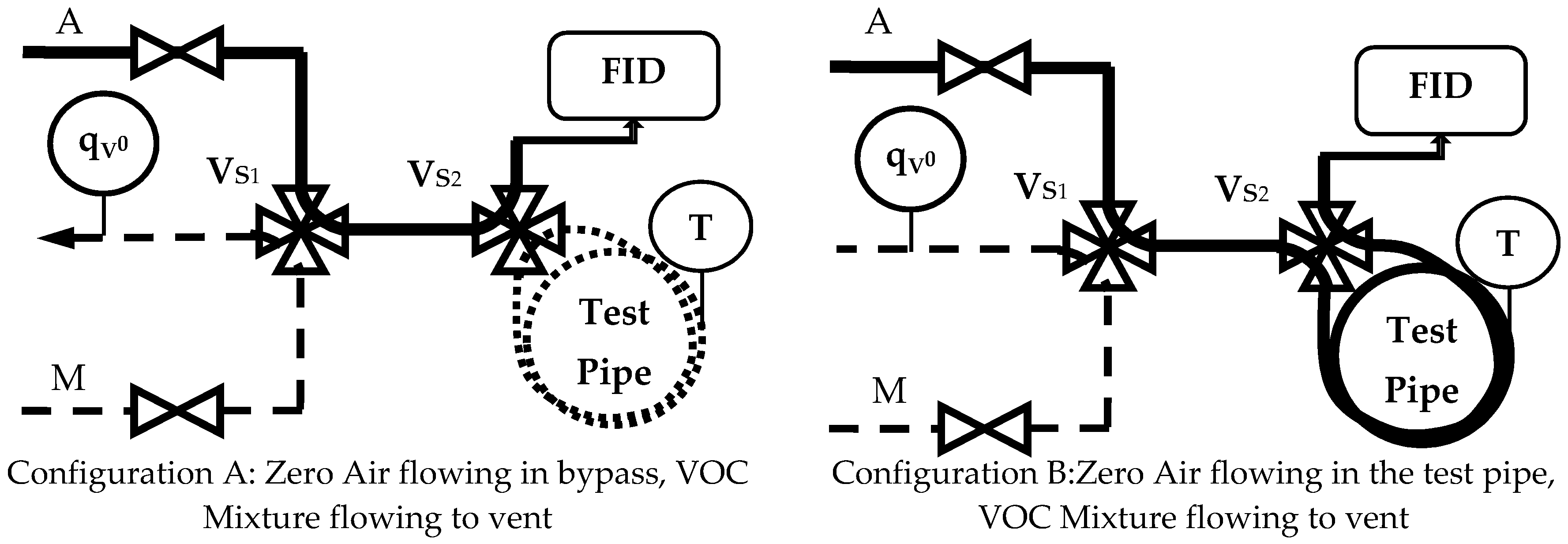
• Configuration A: the detector receives the Zero Air flowing through the bypass while the VOC Mixture is sent to the vent (Ref. Figure 2); gas is entrapped in the test pipe.
• Configuration B: the detector receives the Zero Air flowing through the test pipe while the VOC Mixture is sent to the vent (Ref. Figure 2).
• Configuration C: the detector receives the VOC Mixture flowing through the bypass, while Zero Air is sent to the vent; Zero Air is entrapped in the test pipe.
• Configuration D: the detector receives the VOC Mixtures flowing through the test pipe while Zero Air is sent to the vent.

To switch from Configuration A to C and from B to D and vice versa, valve V_s1 is turned by 90°; to switch from Configuration A to B and from C to D and vice versa, valve V_s2 is turned by 90°.

2.2. Materials

Tests were performed on commercial pipes with 1/8” nominal diameter, internal diameter was measured by weighing pipes empty and filled by water on 1 m pipe length with 0.1% uncertainty. Sulfinert^® coated stainless steel with pipe lengths of 26 ± 0.13 m and 8.5 ± 0.045 m has been tested. Two samples, 8.5 m long, were cut from a Sulfinert^® 26 m pipe. Acetone was chosen as VOC because of its high response on FID and its chemical stability [51], of its very low toxicity, and of its importance in applications [3,5,31]. Acetone at a nominal 10 μmol mol⁻¹ was supplied as a VOC mixture in air from a gas cylinder. Experiments were performed from two cylinders of the same nominal mole fraction (χ = 10 ± 0.3 μmol mol⁻¹, SIAD certified mixture χ = 9.78 ± 0.38 μmol mol⁻¹ and χ = 9.86 ± 0.35 μmol mol⁻¹ Acetone in air.) and the results were compared on tests; the effect on repeatability was negligible. μmol mol⁻¹ level was selected to assure higher stability of the acetone source supplied to the device for cylinder, pressure reducer, and line.

3. Methodology

3.1. Measurand Equation: Amount of VOC Adsorbed Per Unit Area of Wall at Equilibrium

The definition of the measurand is “the amount of VOC adsorbed per unit area of wall at equilibrium”, i.e., the areic amount of VOC (C_A,e) in mol m⁻². It can be calculated by the information about the mixture entering (subscript in) and leaving (subscript out) the test pipe through a simple mass balance for the conservation of VOC, i.e., VOC changes state from free molecule to molecule adsorbed on the wall (VOC (gas) → VOC (wall)), in a cylinder, i.e., the test pipe. The mass balance (in moles) can be written as: “the amount of VOC entering the test pipe per unit time (q_nVOC,in, mol min⁻¹) leaves the test pipe as the amount of VOC exiting the test pipe per unit time (q_nVOC,out, mol min⁻¹) or remains inside the test pipe as the amount of VOC adsorbed on the wall (dn_VOC,wall, mol) in the unit time” or, in a mathematical way:

$$q_{n_{\mathit{VOC}},\mathit{in}}=q_{n_{\mathit{VOC}},\mathit{out}}\left(t\right)+\frac{{\mathit{dn}}_{\mathit{VOC},\mathit{wall}}\left(t\right)}{\mathit{dt}}$$

(2)

The measurand (C_A,e, mol m⁻²) can be calculated from the integral by parts of equation (2) as the integral on time of the difference between the amount entering (q_nVOC,in, mol min⁻¹) and leaving (q_nVOC,out, mol min⁻¹) the test pipe per unit time. The time interval is from clean pipe (t₀) to saturated pipe (t_∞). The amount is referred to the unit area A of the wall to calculate the areic amount of substance at equilibrium:

$$\begin{gathered} C_{A,e}=\frac{n_{\infty }}{A}={{\displaystyle \int }}_0^{n_{\infty }}\frac{{\mathit{dn}}_{\mathit{VOC},\mathit{wall}}\left(t\right)}{A}={{\displaystyle \int }}_{t_0}^{t_{\infty }}\frac{q_{n_{\mathit{VOC}},\mathit{in}}-q_{\mathit{VOC},\mathit{out}}\left(t\right)}{A}\mathit{dt} \\ {C}_{A,e}=\frac{q_{n_{\mathit{VOC}},\mathit{in}}}{A}{{\displaystyle \int }}_{t_0}^{t_{\infty }}\left(1-\frac{q_{n_{\mathit{VOC}},\mathit{out}}\left(t\right)}{q_{n_{\mathit{VOC}},\mathit{in}}}\right)\mathit{dt} \end{gathered}$$

(3)

The areic amount of VOC at the equilibrium is thus the sum (n_∞) of all the aliquots of VOC adsorbed on the wall (n_VOC,wall) moment by moment from the beginning of the exposure till the equilibrium, theoretically till infinitive time (t_∞).

The amount of VOC entering the test pipe (q_nVOC,in, mol min⁻¹) is independent of time and it can be calculated as:

$$q_{n_{VOC},in}= q_{V_g,in} C_{V,in}=q_{V_g^0 }{\chi }_{Mix}\frac{P^0}{R{T}^0}$$

(4)

where C_V,in (mol mL⁻¹) is the mole concentration, i.e., amount concentration, of VOC and q_Vg,in (mL min⁻¹) is the total volumetric gas flow rate feeding the test pipe; χ_Mix (mol mol⁻¹) is the mole fraction, i.e., the amount fraction, of VOC in the mixture and q_V⁰g (SmL min⁻¹) is the total standard volumetric gas flow rate (0 °C, 1 bar), its value is practically uniform along the test pipe, i.e., the amount of VOC segregated at the wall is negligible with respect to the total amount flow rate; T⁰ (K) and P⁰ (kPa) are the temperature and pressure at standard conditions (0 °C, 1 bar) and R (kJ K⁻¹ mol⁻¹) is the gas constant.

While the ratio between the amount flow rate of VOC entering and leaving the test pipe can be expressed as the dimensionless mole fraction of VOC (ζ) as long as the total mole flow rate accounted as standard volumetric flow rate (q_V⁰g) is uniform along the test pipe (in other words as long as the amount of VOC adsorbed is negligible with respect to the total amount of gas). A baseline signal of FID is related to several effects, and to account for all the possible effects, clean air has been flushed in the system [51]. FID signal shift from the baseline is proportional to the total amount of carbon burned in the flame in the unit time, and the response factor is proper of each substance mainly based on the molecular formula [51]. This quantity can be calculated from the signal as:

$$\frac{q_{n_{VOC},\mathit{out}}\left(t\right)}{q_{n_{VOC},\mathit{in}}}=\frac{{\chi }_{out}}{{\chi }_{Mix}}=\zeta \left(t\right)=\frac{S\left(t\right)-S_{Air}}{S_{Mix}-S_{Air}}$$

(5)

where S (mV, in the case of FID) is the signal from the detector when flowing the Zero Air (S_Air), the VOC Mixture from bypass (S_Mix), the gas coming from the test pipe at time t (S(t)). Equation (6) is the final shape of the measurand equation, where ζ is calculated from Equation (5).

$$C_{A,e}=\frac{P^0{q}_{V^0,g}{\chi }_{Mix}}{AR{T}^0}{{\displaystyle \int }}_{t_0}^{t_{\infty }}\left(1-\zeta \left(t\right)\right)dt$$

(6)

During the adsorption (from t₀ to t_∞), the ideal plug flow (ζ = 1) is shifted to the actual dimensionless mole fraction (ζ(t)) because of adsorption, the integral of the difference (1 − ζ(t)) between the ideal dimensionless mole fraction, and the actual one is the amount of adsorption effect in the test pipe.

3.2. Measurement Procedure

The procedure is aimed to get the measurand realization. The test pipe must be cleaned by flushing zero gas (Air) and then exposed to the VOC Mixture over a time interval to measure the VOC uptake. After saturation, the pipe is exposed to the Air over a time interval to measure the VOC release. For cleaning the pipe, configuration B is set till the signal is stabilized at S_Air. After cleaning by Air, the test pipe is isolated from the device and the device is exposed to the VOC Mixture (Switch to configuration A first, and then configuration C) till the signal is stabilized at S_Mix and the device is saturated. Once the stability is reached, the test pipe is exposed to VOC Mixture (Switch to configuration D) till the signal is stabilized again at S_Mix. The procedure results in signal shape, a typical shape is reported in the central part of Figure 3 for 6 repeated measurements.

The procedure is reported in

Table 1. Sequence of configurations on measurement.

Switch	Valve	S∞	Test Pipe		Gas	Operation and Effects
B		SAir	In	Clean	Zero	Cleaning device and test pipe till Flat signal
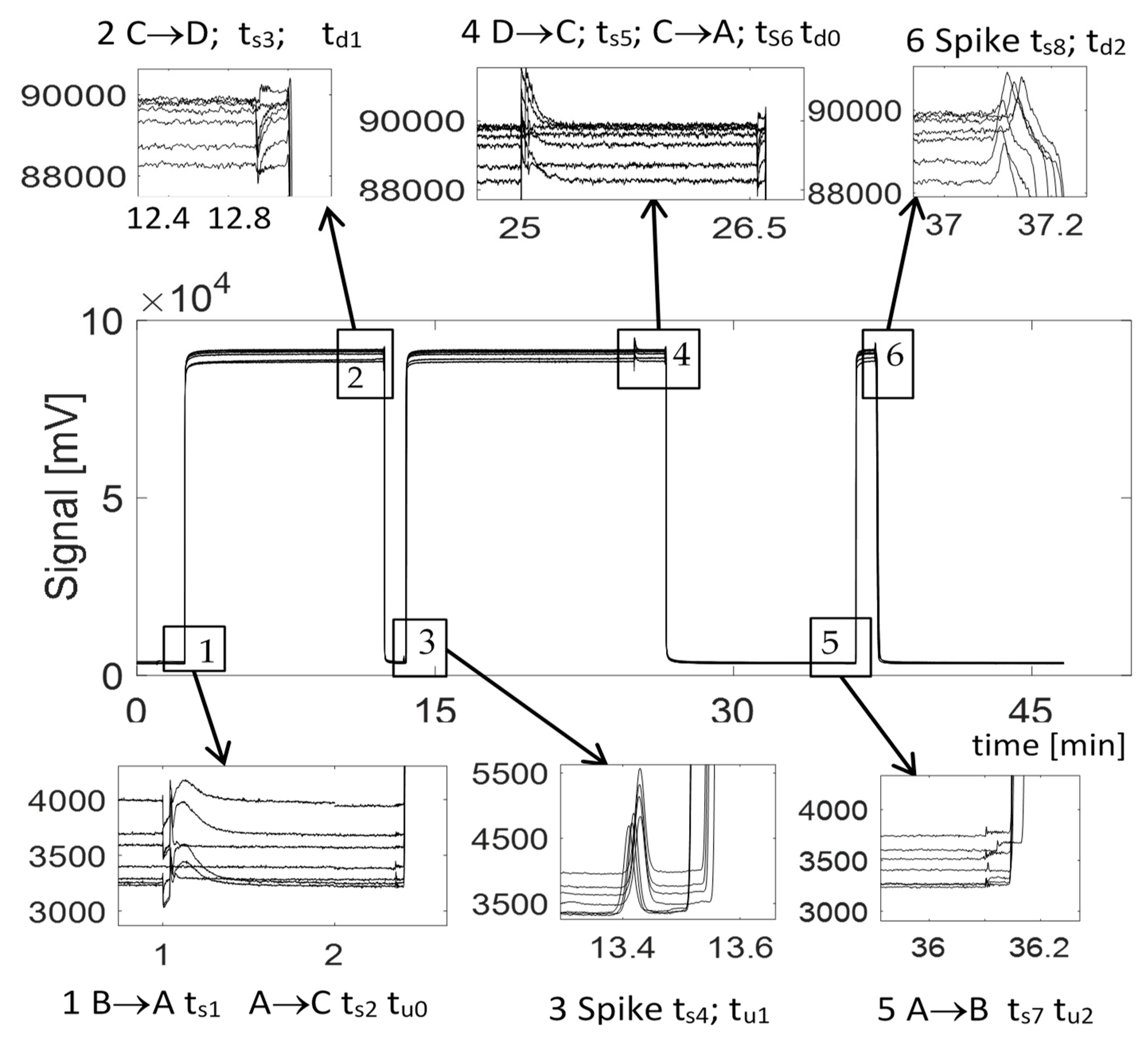
B→A	Vs2	SAir	Off	Clean	Zero	Spike (ts1) at switch
A→C	Vs1	SMix	Off	Clean	VOC	Spike (ts2) at switch, tu0, Saturating device
C→D	Vs2	SMix	In	Sat.	VOC	Spike (ts3) at switch Signal depletion (td1) after device residence time Spike (ts4) after test pipe residence times tu1
D→C	Vs2	SMix	Off	Sat.	VOC	Spike (ts5) at switch, Cleaning device
C→A	Vs1	SAir	Off	Sat.	Zero	Spike (ts6) at switch td0
A→B	Vs2	SAir	In	Clean	Zero	Spike (ts7) at switch Signal increase (tu2) after device residence time Spike (ts8) after test pipe residence times, td1

as the sequence of configurations and switches performed during a single measurement. The procedure is completed with the desorption reaching again the initial conditions after cleaning. The effects reported in Table 1 are deviations from the theoretical signal behavior. Spikes in the signal were observed in correspondence to switches and other occurrences. Delays were observed for the appearance and disappearance of VOC in FID. Figure 3 reports a typical pattern of the signal along a run, the different curves give an idea or repeatability of the experiment. Boxes enlarge the scales of the signal to put in evidence deviations. Spikes identify the time of events from a physical direct measurement.

Table 2. Correspondence of signal times with residence/contact times, box refers to Figure 3.

Time	Box	Event	Characteristic Time
Spike ts1	1	B→A Switch
Spike ts2	1	A→C Switch
tu0	1	VOC Mixture reaches FID	tu0 − ts2 Residence time from Vs1 to detector no test pipe
Spike ts3	2	C→D Switch
td1	2	Air entrapped reaches FID	td1 − ts3 Residence time from Vs2 to detector
Spike ts4	3	VOC Mixture reaches FID without VOC (all adsorbed on wall)	τr = ts4 − td1 Residence time in test pipe
tu1	3	VOC starts to overpass pipe	Delay of VOC appearance
Spike ts5	4	D→C Switch
Spike ts6	4	C→A Switch
td0	4	Zero Air reaches the FID	td0 − ts6 Residence time in the device without test pipe
Spike ts7	5	A→B Switch
tu2	5	VOC Mixture entrapped reaches FID	tu2 − ts7 Residence time from Vs2 to detector
Spike ts8	6	Zero Air reaches FID	τR = ts8 − tu2 Residence time in test pipe
td1	6	VOC starts to overpass pipe	Delay of VOC disappearance

reports the time correspondence and reference to box numbers in Figure 3.

3.3. Bias Correction

The main source of bias comes from the presence of a volume of Zero Air entrapped in the pipe at switch C→D. The first effect of Zero Air entrapped is to create a depletion in the signal which modifies the integral (I) of dimensionless mole fraction (ζ) by a quantity that is theoretically equal to the residence time (I = (ζ_Mix − ζ_Air)τ_R = (1 − 0)τ_{R =} τ_R)). The effect starts when the air entrapped reaches the FID (t_d1) and has a duration equal to the residence time (τ_R = t_s4 − t_d1). The second effect is the desorption from the part of the device that connects the test pipe to the detector. This part is saturated by VOC at the V_s2 switch time. The effect acts while the air entrapped in the pipe at the V_s2 switch time (t_s1) is crossing that part of the system. The second effect starts to act when the air entrapped reaches the FID (t_d1), i.e., the V_s2 switch time plus the residence time in the part, and has a duration equal to the residence time in the test pipe (τ_R = t_s4 − t_d1). A third effect is the adsorption of the same part of the system that is saturated again while the signal raises up. The third effect starts to act when the gas mixture reaches the FID detector after the V_s2 switch (t_s4) and is persisting till saturation of the part. This results in a bias on the integral, the second and the third effects are equal and opposite.

Thus, the bias can be corrected by subtracting the residence time in the test pipe (first line of Equation (7)) or splitting the integral (I) in desorption (I_des) in the interval (from t_d1 to t_s4) and adsorption (I_ads) in the interval (from t_s4 to t_∞) (second line of Equation (7)). In both intervals, the difference is between the ideal plug flow and the effective signal. During the desorption interval (from t_d1 to t_s4), the gas entrapped in the pipe at t_s1 desorbs the VOC from the connection between the test pipe and the detector and modifies the dimensionless mole fraction from the ideal Zero Air (ζ = 0) entrapped to the actual dimensionless mole fraction (ζ), the integral of the difference (0 − ζ) between the ideal dimensionless mole fraction, and the actual one is the amount of desorption effect in the connection between the test pipe and the detector. While in the adsorption interval (from t_s4 to t_∞), the ideal VOC Mixture plug flow (ζ = 1) is shifted to the actual dimensionless mole fraction (ζ) because of the adsorption, the integral of the difference (1 − ζ) between the ideal dimensionless mole fraction, and the actual one is the amount of adsorption effect in the test pipe and in the connection between the test pipe and the detector. The sum of the two integrals is the adsorption effect in the test pipe only.

$$\begin{gathered} I={{\displaystyle \int }}_{t_0}^{t_{\infty }}\left[1-\zeta \left(t\right)\right]dt-{\tau }_r \\ I={{\displaystyle \int }}_{t_{d1}}^{t_{s4}}\left[0-\mathsf{\zeta }\left(t\right)\right]\mathit{dt}+{{\displaystyle \int }}_{t_{s4}}^{t_{\infty }}\left[1-\mathsf{\zeta }\left(t\right)\right]\mathit{dt}=I_{\mathit{des}}+I_{\mathrm{ads}} \end{gathered}$$

(7)

The second approach resulted in much more reproducible and was used in this paper. The measurand equation (Equation (6)) with bias correction becomes:

$$C_{A,e}=\frac{P^0}{R{T}^0}\frac{q_{V_g^0}{\chi }_{Mix}}{A}\left(I_{des}+I_{ads}\right)$$

(8)

To make the signals explicit, Equation (8) is transformed in:

$$C_{A,e}=\frac{P^0}{{\mathit{RT}}^0}\frac{q_{V_g^0}{\chi }_{\mathit{Mix}}}{A}\left[{{\displaystyle \int }}_{t_{d1}}^{t_{s4}}\frac{S_{\mathit{Air}}-S\left(t\right)}{S_{\mathit{Mix}}-S_{\mathit{Air}}}\mathit{dt}+{{\displaystyle \int }}_{t_{s4}}^{t_{\infty }}\frac{S_{\mathit{Mix}}-S\left(t\right)}{S_{\mathit{Mix}}-S_{\mathit{Air}}}\mathit{dt}\right]$$

(9)

The same reasoning can be applied to the desorption section of the experiment to calculate the areic desorbed amount corrected for the bias that comes from the VOC Mixture entrapped in the pipe at switch A→B to calculate the measurand. During the adsorption interval (from t_u2 to t_s8), the gas entrapped in the pipe at t_s5 adsorbs the VOC to the connection between the test pipe and the detector and modifies the dimensionless mole fraction from the ideal VOC Mixture (ζ = 1) entrapped to the actual dimensionless mole fraction (ζ), the integral of the difference (1 − ζ) between the ideal dimensionless mole fraction, and the actual one is the amount of adsorption effect in the connection between the test pipe and the detector. While in the desorption interval (from t_s8 to t_∞), the ideal Zero Air plug flow (ζ = 0) is shifted to the actual dimensionless mole fraction (ζ) because of the desorption, the integral of the difference (0 − ζ) between the ideal dimensionless mole fraction, and the actual one is the amount of desorption effect in the test pipe and in the connection between the test pipe and the detector. The sum of the two integrals is the desorption effect in the test pipe only.

$$\begin{gathered} I={{\displaystyle \int }}_{t_{u2}}^{t_{s8}}\left[1-\mathsf{\zeta }\left(t\right)\right]\mathit{dt}+{{\displaystyle \int }}_{t_{s8}}^{t_{\infty }}\left[0-\mathsf{\zeta }\left(t\right)\right]\mathit{dt}+=I_{ads}+I_{\mathit{des}} \\ {C}_{A,e}=\frac{P^0}{{\mathit{RT}}^0}\frac{q_{V_g^0}{\chi }_{\mathit{Mix}}}{A}\left[{{\displaystyle \int }}_{t_{u2}}^{t_{s8}}\frac{S_{\mathit{Mix}}-S\left(t\right)}{S_{\mathit{Mix}}-S_{\mathit{Air}}}\mathit{dt}+{{\displaystyle \int }}_{t_{s8}}^{t_{\infty }}\frac{S_{\mathit{Air}}-S\left(t\right)}{S_{\mathit{Mix}}-S_{\mathit{Air}}}\mathit{dt}\right] \end{gathered}$$

(10)

Other possible sources of bias are the interactions with different parts of the system. Valves and pressure reducers are the main sources of uncertainty. Valves have internal surfaces uncoated that can react with Acetone, reducing the accuracy of the method. Pressure reducers have membranes that can release substances that interfere with the detector signal. This paper is aimed to verify the reproducibility of the method. The method is based on the difference between detector response with and without test pipe. It means that the reproducible effects are not interfering with the purpose of the paper because they are canceled by the difference. To assure a higher reproducibility, a single amount fraction has been used to improve the reproducibility of irreversible first-order interactions in the valves. The high amount of substance fraction has been selected to reduce the weight of the release from pressure reducers, improving reproducibility. Pressure reducers play an important role when the method is applied at low amount fraction investigation.

4. Results

Tests were performed with a sample of Sulfinert^® pipe as a whole and cut in 2 subsamples of the same lengths to verify the effects of operating conditions and to verify the reproducibility on samples. Tests were performed at different residence times, flow rates, Reynolds numbers, and temperatures, at atmospheric pressure (plus pressure drop). The ranges of test conditions are reported in

Table 3. Sulfinert^® Number of experiments, pipe lengths, and test condition ranges (residence time, temperature, pressure, and Reynolds number.

Sample	N	L	qV0g	τr	T	P	Re
		(m)	(SmL min−1)	(min)	(°C)	(kPa)	(-)
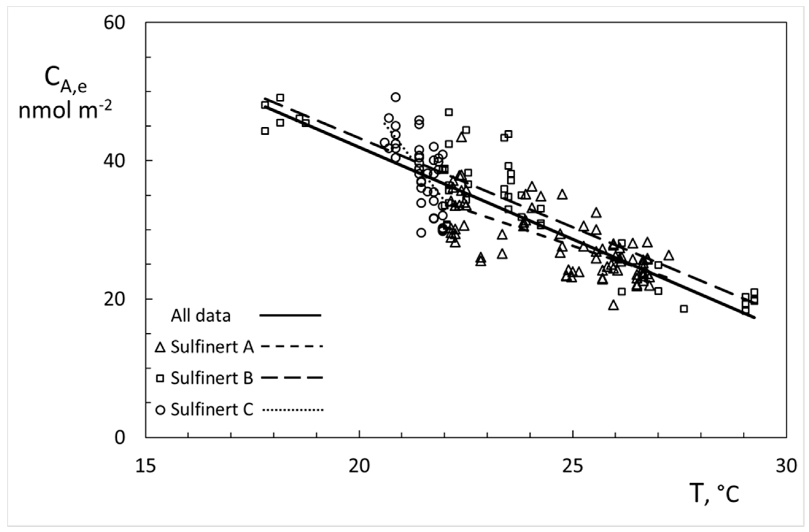
Sulfinert A	53	26	9–195	0.5–9.5	22–27	100–130	5–150
Sulfinert B	29	8.5	9–55	0.6–3.2	17–30	100–120	5–40
Sulfinert C	18	8.5	9–55	0.6–3.2	20–22	100–120	5–40

. Tests were repeated on each sample. Data from samples A, B, and C as mean values and mean square deviation of raw data are reported in

Table 4. Sulfinert^® Areic amount adsorbed (C_A,e). Raw data and data corrected at 20 °C 1 bar with experimental standard deviations for a single sample and all data aggregated.

Sample	CA,e	σ	σ%	CA,e, 20 °C, 1 bar	σ, 20 °C, 1 bar	σ%. 20 °C, 1 bar
	(nmol m−2)	(nmol m−2)	σ/CA,e	(nmol m−2)	(nmol m−2)	σ/CA.e
Sulfinert A	28.2	4.8	17%	38.2	2.8	7.3%
Sulfinert B	34.0	9.1	27%	41.7	3.3	8.0%
Sulfinert C	38.5	4.9	13%	39.6	3.4	8.5%
All data	32.3	7.6	24%	39.5	3.4	8.6%
Mean ABC	33.5	5.2	15%	39.8	1.7	4.4%

.

Data were tested in a range of temperature and pressure due to the room conditions and pressure drop in the device. The three samples are considered as a unique population with respect to temperature and pressure dependency of interaction phenomena as well as the adsorption and the desorption datasets. Welch statistical t-tests cannot reject the hypothesis that all data belong to a unique population with a confidence of 95%.

The temperature was calculated as the mean of temperature measured on the external surface of the test pipe along the run time in a different position along the test pipe. A sensitivity coefficient of 2.66 ± 0.12 nmol m⁻² K⁻¹ was calculated for the temperature (Figure 4) as the slope of the linear regression curve on the whole dataset from the three samples. A different slope was observed for each sample, this is mainly due to the different range of temperature and it is particularly evident in the sample C dataset with a range of temperature of 2 K against 5 K for sample A and 13 K for sample B. Data were corrected for the temperature bias at 20 °C.

The pressure was calculated as the mean of maximum and minimum ambient pressure observed during the run added the mean of pressure drop with and without the test pipe, i.e., an estimation of the average pressure along the test pipe. A sensitivity coefficient of 237 ± 31 nmol m⁻² MPa⁻¹ for the pressure (Figure 5) as the slope of the linear regression curve on the whole dataset from the three samples, for data corrected for temperature bias. A different slope was observed for each sample. Data were corrected also for the pressure bias at 1 bar as reported in Table 4.

Table 4 reports the standard deviation (σ) over the datasets including adsorption and desorption values. Lines account for different datasets: single datasets, all the data in one set, and considering samples A, B, and C separately as single data. The variability of data is reduced by the correction of biases depending on the wideness of the temperature and pressure ranges in the specific datasets.

Figure 6 shows the plot of average values of the three samples grouped at 6 different Reynolds Number (Re) in order to check a dependency of the adsorbed amount on the fluid dynamic effects inside the pipe. Re was always lower than 200 so a laminar regime always occurred in the test pipes. A slope of −0.013 ± 0.006 nmol m⁻² was calculated by linear regression on all the data and −0.018 ± 0.010 nmol m⁻² by linear regression on the mean values, the resulted curves are not plotted in Figure 6 because they are not evidently different from the line of the mean value. The deviation from the mean value was lower than variability on the whole range of Re, and the effect of the slope on the whole range was observed to be lower than the variability of each data subset. Upper and lower lines in Figure 6 and Figure 7 are the envelopes of all data, max and minimum values have an opposite trend against Re. In conclusion, Re does not affect the amount of Acetone adsorbed per unit area of the pipe wall.

Figure 7 show the plot of average values of the three samples grouped at 5 different residence time in order to check a dependency of the adsorbed amount on the contact time. Contact time ranged between 0.5 and 9 min for all the samples. A slope of −0.46 ± 0.12 nmol m⁻² min⁻¹ was calculated by linear regression on all the data and −0.57 ± 0.13 nmol m⁻² min⁻¹ by linear regression on the mean values. The variability of the mean values seems lower for residence time lower than 4 min. The upper and lower lines in Figure 7 are the envelope of all data, minimum values have a flat trend against the residence time. The effect of residence time on the adsorbed amount per unit area is not completely clear but, in any case, very limited.

The longer sample, sample A, was the only one working at a high Reynolds number (more than 50) and at a high residence time (more than 4 min). Both in Figure 6 and Figure 7 a lower value is observed, much more evident in Figure 7. Since the average value of sample A is lower (Table 4), the effect of the sample could be the only relevant on differences.

The comparison of adsorption and desorption runs allows analyzing the reversibility of the interactions. The difference between the amounts of Acetone that disappeared in the first part of the run and appeared in the second part of the run was calculated to be 1.5 ± 0.33 nmol m⁻² as the difference of the mean values corrected for the temperature and pressure biases and 2.3 ± 0.53 nmol m⁻² as the mean of the differences measured in each run. Reproducibility was calculated as the standard deviation of the mean.

5. Discussion

The measurand was defined and realized by the mass balance of VOC across the test pipe. An experimental device was specially designed to improve the reproducibility of experiments in data production even without a narrow control of temperature and pressure. The flow rate was kept under control by sonic nozzles and inlet pressure regulation as mass flow rate, volumetric flow rates, and pressures were kept reproducible regulating pressure drops by capillary pipes in both vent and detector lines. Four-way switch crossover valves were used to reduce the area of bypass and to make switches by a unique movement to change from zero gas to the VOC mixtures (Acetone) and to insert and from bypass to the test pipe. Biases were corrected accounting for desorption in the line that connects the test pipe to the detector.

The extent of the range of temperature, mainly due to the seasonal variations, was around 10 K and a correction was necessary to compare data, a sensitivity factor on temperature was calculated. The extent of the range of pressure, mainly due to the pressure drop under different operational conditions, was around 30 kPa and a correction was necessary to compare data, a sensitivity factor on pressure was calculated.

Table 5. Sulfinert^® specific amount adsorbed (C_A,e) and equilibrium constant (K_e). Data were corrected at 20 °C 1 bar. Reproducibility as the experimental standard deviation of the mean of corrected data. Single Sulfinert^® samples A, B, C, all data sets in one and calculated from the samples.

Sample	CA,e,20 °C,1 bar	σ20 °C,1 bar	σ%,20 °C,1 bar	Ke,20 °C,1 bar	σ,20 °C,1 bar	σ%,20 °C,1 bar
	(nmol m−2)	(nmol m−2)	σ/CA,e	(m)	(m)	σ/Ke
Sulfinert A	38.2	0.3	0.8%	0.173	0.002	1.0%
Sulfinert B	41.7	0.5	1.2%	0.185	0.003	1.5%
Sulfinert C	39.6	0.5	1.3%	0.171	0.002	1.4%
All data	39.5	0.3	0.7%	0.176	0.001	0.8%
Mean ABC	39.8	1.0	2.5%	0.176	0.005	2.6%

reports mean values and standard deviation of the mean for single datasets, for all the data in one set and considering samples A B and C separately as single data in order to compare the reproducibility of the method and to focus on the difference between samples. The standard deviation of the mean of the dataset with data corrected for temperature and pressure is considered as the total uncertainty of the measurement [53]. The value is very small around 1%, this could mainly due to the characteristic of Sulfinert^® coating on stainless steel that assures very low irreversible interferences and no permeation into the pipe wall limiting the instability of measurand. A poorer reproducibility is expected with polymeric materials or uncoated metals. This result candidate the method for quality control of the coating by a reference procedure.

The same reproducibility among samples 1.00 nmol m⁻² was calculated as uniform distribution of probability between the maximum and minimum observed values, and as the normal distribution of probability, i.e., the standard deviation of the mean of the three values. Reproducibility between samples is around 2.5% of the value calculated as Type A uncertainty [53].

If a linear equation is used to describe the equilibrium condition between a VOC mixture and the pipe internal surface, the equilibrium constant can be calculated as the ratio between the areic mole of VOC (C_A,e) on the wall surface and the mole concentration in the gas mixture at the equilibrium (C_V,e) [30]:

$$K_e=\frac{C_{A,e}}{C_{V,e}}$$

(11)

The measured values are reported in the last columns of Table 5. As expected, the constant does not depend on the fluid dynamic conditions (Re) and on the contact time between the VOC Mixture and the pipe, the constant value depends on temperature and pressure.

6. Conclusions

Uncertainty of VOC measurements at ppb level is affected by the interactions of gas mixtures with the sampling lines especially when concentration is at trace levels. A key topic is the quantification of the loss amount that can be considered as a bias for the measurement of the amount of VOC. The method here proposed is an experimental quantification of interactions that reaches an equilibrium between a gas mixture and a pipe wall. Even if the actual quantification is at ppm level, due to the available VOC mixture source and the available detector, the method is applicable in principle to lower concentration levels depending on the availability of a mixture source and a detector. The ppm level assures a good reproducibility and has insights to lower levels if the interaction mechanisms remain the same as expected.

The device allowed to have good control of the experiment. The 4-way valves are really effective in switches giving a limited disturbance on pressure and signal and minimize the surface area in the bypass. Sonic nozzles allowed good stability to the flow rates being independent of the discharge pressure. The control of temperature and pressure was not critical, even if it was really very broad. The estimation of average temperature and pressure inside the test pipe was effective for the calculation of the biases. The method can be applied to compare different materials or scenarios, or to investigate competition between substances, e.g., with moisture. In the last case, the mutual effects of substances on detectors and mixture generators can be critical. The method is actually under investigation at a very low level of amount of substance (ppb) with a PTR-MS as a detector, with acetone, methanol, and ethanol as VOCs and at different levels of moisture.

References

- Sassi, G.; Demichelis, A.; Lecuna, M.; Sassi, M.P. Preparation of standard VOC mixtures for climate monitoring. Int. J. Environ. Anal. Chem. 2015, 95, 1195–1207. [Google Scholar] [CrossRef]
- Investigations for the Improvement of the Measurement of Volatile Organic Compounds from Floor Coverings within the Health-Related Evaluation of Construction Products. Available online: https://www.google.com.sg/url?sa=t&rct=j&q=&esrc=s&source=web&cd=&cad=rja&uact=8&ved=2ahUKEwj7wPb9wujuAhW5yYsBHSoFD_kQFjABegQIBBAC&url=https%3A%2F%2Fopus4.kobv.de%2Fopus4-bam%2Ffiles%2F19838%2FInvestigations%2Bfor%2Bthe%2Bimprovement%2Bof%2Bthe%2Bmeasurement%2Bof%2Bvolatile%2Borganic%2Bcompounds%2Bfrom%2Bfloor%2Bcoverings%2Bwithin%2Bthe%2Bhealth-related%2Bevaluation%2Bof%2Bconstruction%2Bproducts.pdf&usg=AOvVaw2zTZtBrY2SQkxJekU3Qu9r (accessed on 27 January 2021).
- Penkett, S. GAW Report No. 171: A WMO/GAW Expert Workshop on Global Long-Term Measurements of Volatile Organic Compounds (VOCs); World Meteorological Organization (WMO): Geneva, Switzerland, 2007. [Google Scholar]
- Rappengluck, B.; Apel, E.; Bauerfeind, M.; Bottenheim, J.; Brickell, P.; Cavolka, P.; Cech, J.; Gatti, L.; Hakola, H.; Honzak, J.; et al. The first VOC intercomparison exercise within the Global Atmosphere Watch (GAW). Atmos. Env. 2006, 20, 7508–7527. [Google Scholar] [CrossRef]
- Pascale, C. 19ENV06, MetClimVOC, Metrology for Climate Relevantvolatile Organic Compounds. European Metrology Programme for Innovation AndResearch (EMPIR). 2019. Available online: https://www.aramis-r.admin.ch/Kategorien/?ProjectID=47398&Sprache=en-US (accessed on 27 January 2021).
- Roberts, M.; Reiss, M.; Monger, G. Advanced Biology; Nelson Thornes: Cheltenham, UK, 2000. [Google Scholar]
- Rovelli, S.; Cattaneo, A.; Fazio, A.; Spinazzè, A.; Borghi, F.; Campagnolo, D.; Dossi, C.; Cavallo, D.M. VOCs Measurements in Residential Buildings: Quantification via Thermal Desorption and Assessment of Indoor Concentrations in a Case-Study. Atmosphere 2019, 10, 57. [Google Scholar] [CrossRef] [Green Version]
- De Gennaro, G.; Farella, G.; Marzocca, A.; Mazzone, A.; Tutino, M. Indoor and outdoor monitoring of volatile organic compounds in school buildings: Indicators based on health risk assessment to single out critical issues. Int. J. Environ. Res. Public Health 2013, 10, 6273–6291. [Google Scholar] [CrossRef] [PubMed]
- Adgate, J.; Church, T.; Ryan, A.; Ramachandran, G.; Fredrickson, A.; Stock, T.; Morandi, M.; Sexton, K. Outdoor, indoor, and personal exposure to VOCs in children. Environ. Health Perspect. 2004, 112, 1386–1392. [Google Scholar] [CrossRef] [PubMed] [Green Version]
- Demichelis, A.; Sassi, G.; Lecuna, M.; Sassi, M. Molar fraction stability in dynamic preparation of reference trace gas mixtures. IET Sci. Meas. Technol. 2016, 10, 414–419. [Google Scholar] [CrossRef]
- Vogt, S.R.; Landoni, C. Approaches to airborne molecular contamination assessment. In Metrology, Inspection, and Process Control for Microlithography XXV; SPIE: Washington, DC, USA, 2011. [Google Scholar]
- Hattori, T. Chemical Contamination Control in ULSI Wafer Processing. 2001. Available online: https://aip.scitation.org/doi/pdf/10.1063/1.1354411 (accessed on 27 January 2021).
- Gordon, S.M.; Szidon, J.P.; Krotoszynski, B.K.; Gibbons, R.D.; O’Neill, H.J. Volatile organic compounds in exhaled air from patients with lung cancer. Clin. Chem. 1985, 31, 1278–1282. [Google Scholar] [CrossRef] [PubMed]
- Peng, G.; Tisch, U.; Adams, O.; Hakim, M.; Shehada, N.; Broza, Y.Y.; Billan, S.; Abdah-Bortnyak, R.; Kuten, A.; Haick, H. Diagnosing lung cancer in exhaled breath using gold nanoparticles. Nat. Nanotechnol. 2009, 4, 669–673. [Google Scholar] [CrossRef] [PubMed]
- Wang, C.; Dong, R.; Wang, X.; Lian, A.; Chi, C.; Ke, C.; Guo, L.; Liu, S.; Zhao, W.; Xu, G. Exhaled volatile organic 16ompound sas lung cancer biomarkers during one-lung ventilation. Sci. Rep. 2014, 4, 1–8. [Google Scholar]
- Adiguzel, Y.; Kulah, H. Breath sensors for lung cancer diagnosis. Biosens. Bioelectron. 2015, 65, 121–138. [Google Scholar] [CrossRef] [PubMed]
- Daneshkhah, A.; Siegel, A.P.; Agarwal, M. Volatile organic compounds: Potential biomarkers for improved diagnosis and monitoring of diabetic wounds. In Wound Healing, Tissue Repair, and Regeneration in Diabetes; Elsevier: Amsterdam, The Netherlands, 2020; pp. 491–512. [Google Scholar]
- Rhoderick, G.C.; Cecelski, C.E.; Miller, W.R.; Worton, D.R.; Moreno, S.; Brewer, P.J.; Viallon, J.; Idrees, F.; Moussay, P.; Kim, Y.D.; et al. Stability of gaseous volatile organic compounds contained in gas cylinders with different internal wall treatments. Elementa 2019, 7, 28. [Google Scholar] [CrossRef] [Green Version]
- Brewer, P.; Brown, R.; Mussell, E.; van Aswegen, S.; Ward, M.; Hill-Pearce, R.; Worton, D. Breakthrough in Negating the Impact of Adsorption in Gas Reference Materials. Anal. Chem. 2019, 91, 5310–5315. [Google Scholar] [CrossRef]
- Pagonis, D.; Krechmer, J.E.; De Gouw, J.; Jimenez, J.L.; Ziemann, P.J. Effects of gas–wall partitioning in Teflon tubing and instrumentation on time-resolved measurements of gas-phase organic compounds. Atmos. Meas. Tech. 2017, 10, 4687–4696. [Google Scholar] [CrossRef] [Green Version]
- Yeh, G.K.; Ziemann, P.J. Gas-wall partitioning of oxygenated organic compounds: Measurements, structure–activity relationships, and correlation with gas chromatographic retention factor. Aerosol Sci. Tech. 2015, 49, 727–738. [Google Scholar] [CrossRef]
- Krechmer, J.E.; Pagonis, D.; Ziemann, P.J.; Jimenez, J.L. Quantification of gas-wall partitioning in Teflon environmental chambers using rapid bursts of low-volatility oxidized species generated in situ. Environ. Sci. Tech. 2016, 50, 5757–5765. [Google Scholar] [CrossRef] [PubMed]
- Ye, P.; Ding, X.; Hakala, J.; Hofbauer, V.; Robinson, E.S.; Donahue, N.M. Vapor wall loss of semi-volatile organic compounds in a Teflon chamber. Aerosol Sci. Tech. 2016, 50, 822–834. [Google Scholar] [CrossRef] [Green Version]
- Huang, Y.; Zhao, R.; Charan, S.M.; Kenseth, C.M.; Zhang, X.; Seinfeld, J.H. Unified Theory of Vapor–Wall Mass Transport in Teflon-Walled Environmental Chambers. Environ. Sci. Tech. 2018, 52, 2134–2142. [Google Scholar] [CrossRef] [Green Version]
- Arrhenius, K.; Fischer, A.; Büker, O. Methods for sampling biogas and biomethane on adsorbent pipes after collection in gas bags. Appl. Sci. 2019, 9, 1171. [Google Scholar] [CrossRef] [Green Version]
- Liu, X.; Deming, B.; Pagonis, D.; Day, D.A.; Palm, B.B.; Talukdar, R.; Roberts, J.M.; Veres, P.R.; Krechmer, J.E.; Thornton, J.A.; et al. Effects of gas–wall interactions on measurements of semivolatile compounds and small polar molecules. Atmos. Meas. Tech. 2019, 12, 3137–3149. [Google Scholar] [CrossRef] [Green Version]
- McMurry, P.H.; Grosjean, D. Gas and aerosol wall losses in Teflon film smog chambers. Environ. Sci. Tech. 1985, 19, 1176–1182. [Google Scholar] [CrossRef]
- McCabe, W.; Smith, J.; Harriott, P. Unit Operations of Chemical Engineering; McGraw Hill: New York, NY, USA, 1956. [Google Scholar]
- Zhang, J.; Zhang, J.; Chen, Q.; Yang, X. A critical review on studies of volatile organic compound (VOC) sorption by building materials (RP-1097). Trans. Am. Soc. Heat. Refriger. Air Cond. Eng. 2001, 108, 162–174. [Google Scholar]
- Goss, K.-U. The air/surface adsorption equilibrium of organic compounds under ambient conditions. Crit. Rev. Environ. Sci. Tech. 2004, 34, 339–389. [Google Scholar] [CrossRef]
- Metrology for VOC Indicators in Air Pollution and Climate Change. Euramet European Metrology Research Programme (EMRP). 2013. Available online: https://www.era-learn.eu/network-information/networks/emrp/emrp-call-2013-energy-and-environment/metrology-for-voc-indicators-in-air-pollution-and-climate-change (accessed on 27 January 2021).
- Nowak, J.; Neuman, J.; Kozai, K.; Huey, L.; Tanner, D.; Holloway, J.; Ryerson, T.; Frost, G.; McKeen, S.; Fehsenfeld, F. A chemical ionization mass spectrometry technique for airborne measurements of ammonia. J. Geophys. Res Atmos. 2007, 112, D10. [Google Scholar] [CrossRef]
- Neuman, J.A.; Huey, L.G.; Ryerson, T.B.; Fahey, D.W. Study of inlet materials for sampling atmospheric nitric acid. Environ. Sci. Tech. 1999, 33, 1133–1136. [Google Scholar] [CrossRef]
- World Meteorological Organization (WMO). Standard Operating Procedures (SOPs) for Air Sampling in Stainless Steel Canisters for Non-Methane. 2012. Available online: https://library.wmo.int/index.php?lvl=notice_display&id=13702#.YCjHezLiuUk (accessed on 27 January 2021).
- Ma, C.; Haider, A.M.; Shadman, F. Atmospheric pressure ionization mass spectroscopy for the study of permeation in polymeric tubing. IEEE Trans. Semicond. Manuf. 1993, 6, 361–366. [Google Scholar] [CrossRef]
- Matsunaga, A.; Ziemann, P.J. Gas-wall partitioning of organic compounds in a Teflon film chamber and potential effects on reaction product and aerosol yield measurements. Aerosol Sci. Tech. 2010, 44, 881–892. [Google Scholar] [CrossRef]
- Lee, S.; Kim, M.E.; Oh, S.H.; Kim, J.S. Determination of physical adsorption loss of primary standard gas mixtures in cylinders using cylinder-to-cylinder division. Metrologia 2017, 54, L26. [Google Scholar] [CrossRef] [Green Version]
- Langmuir, I. The adsorption of gases on plane surfaces of glass, mica and platinum. J. Am. Chem. Soc. 1918, 40, 1361–1403. [Google Scholar] [CrossRef] [Green Version]
- Sassi, G.; Demichelis, A.; Sassi, M.P. Uncertainty analysis of the diffusion rate in the dynamic generation of volatile organic compound mixtures. Meas. Sci. Tech. 2011, 22, 105104. [Google Scholar] [CrossRef]
- Takahashi, C.; Kato, K.; Maruyama, M.; Kim, J.S.; Kao, M.-J.; Botha, A.; Dimashki, M. Final report on key comparison APMP. QM-K4 of ethanol in air. Metrologia 2003, 40, 08008. [Google Scholar] [CrossRef]
- Kato, K.; Maruyama, M.; Kim, J.S.; Hyub, O.S.; Woo, J.-C.; Kim, Y.; Bae, H.; Han, Q.; Zhou, Z. Final report on key comparison APMP. QM-K4. 1: Ethanol in nitrogen. Metrologia 2007, 45, 08007. [Google Scholar] [CrossRef]
- Guenther, F.R.; Miller, W.R.; Duewer, D.L.; Heo, G.S.; Kim, Y.-D.; van der Veen, A.M.H.; Konopelko, L.; Kustikov, Y.; Shor, N.; Brookes, C.; et al. International Comparison CCQM-K41: Hydrogen sulfide in nitrogen. Metrologia 2007, 44, 08004. [Google Scholar] [CrossRef]
- Kim, Y.-D.; Heo, G.-S.; Lee, S.; Han, Q.; Wu, H.; Konopelko, L.A.; Kustikov, Y.A.; Malginov, A.V.; Gromova, E.V.; Pankratov, V.V.; et al. Final report on international key comparison APMP. QM-K41: 10 μmol/mol hydrogen sulfide in nitrogen. Metrologia 2014, 51, 08012. [Google Scholar] [CrossRef]
- Van der Veen, M.H.; Nieuwenkamp, G.; Wessel, R.M.; Maruyama, M.; Heo, G.S.; Kim, Y.-D.; Moon, D.M.; Niederhauser, B.; Quintilii, M.; Milton, M.J.T.; et al. International comparison CCQM K46—Ammonia in nitrogen. Metrologia 2010, 47, 08023. [Google Scholar] [CrossRef]
- Brown, A.S.; Milton, M.; Brookes, C.; Vargha, G.; Downey, M.; Uehara, S.; Augusto, C.; de Lima Fioravante, A.; Sobrinho, D.; Dias, F.; et al. Final report on CCQM-K93: Preparative comparison of ethanol in nitrogen. Metrologia 2013, 50, 08025. [Google Scholar] [CrossRef]
- Lee, S.; Heo, G.S.; Kim, Y.; Oh, S.; Han, Q.; Wu, H.; Konopelko, L.A.; Kustikov, Y.A.; Kolobova, A.V.; Efremova, O.V.; et al. International key comparison CCQM-K94: 10 μmol/mol dimethyl sulfide in nitrogen. Metrologia 2016, 53, 08002. [Google Scholar] [CrossRef]
- Harris, P.; Pelligrini, M. Mass Transport in Sample Transport lines Adsorption Desorption Effects and their Influence on Process Analytical Measurements. Available online: https://www.silcotek.com/hubfs/Literature%20Catalog/White%20Papers/Externally%20Written/Sulfur%20and%20H2S/%23WP-EXT-SULF-002%20ISA%202011%20Sample%20Lines.pdf (accessed on 27 January 2021).
- Deming, L.; Pagonis, D.; Liu, X.; Day, D.A.; Talukdar, R.; Krechmer, J.E.; de Gouw, J.A.; Jimenez, J.L.; Ziemann, P.J. Measurements of delays of gas-phase compounds in a wide variety of tubing materials due to gas–wall interactions. Atmos. Meas. Tech. 2019, 12, 3453–3461. [Google Scholar] [CrossRef] [Green Version]
- Metrology for Airborne Molecular Contamination in Manufacturing Environments. European Metrology Research Programme (EMRP). 2012. Available online: https://www.euramet.org/index.php?eID=tx_securedownloads&p=588&u=0&g=0&t=1641528179&hash=31fb1f3ab963204de5ce80ba65fc8605b53c7edf&file=Media/docs/EMRP/JRP/JRP_Summaries_2012/Industry_SRTs/SRT-i17.pdf (accessed on 27 January 2021).
- Barwood, G. 17IND09, MetAMCII, Metrology for Airborne Molecular Contaminants II European. Metrology Programme for Innovation and Research (EMPIR). 2017. Available online: https://www.era-learn.eu/network-information/networks/empir/empir-call-2017/metrology-for-airborne-molecular-contaminants-ii (accessed on 27 January 2021).
- Szulejko, J.; Kim, Y.H.; Kim, K.H. Method to predict gas chromatographic response factors for the trace-level analysis of volatile organic compounds based on the effective carbon number concepts. J. Sep. Sci. 2013, 36, 3356–3365. [Google Scholar] [CrossRef]
- University of Torino. Meteorological Station of the Department of Physics. 2020. Available online: http://www.meteo.dfg.unito.it/tutti (accessed on 27 January 2021).
- Evaluation of Measurement Data—Guide to the Expression of Uncertainty in Measurement (GUM) JCGM 100:2008. Available online: https://www.bipm.org/utils/common/documents/jcgm/JCGM_100_2008_E.pdf (accessed on 27 January 2021).