Review on Atmospheric Ozone Pollution in China: Formation, Spatiotemporal Distribution, Precursors and Affecting Factors

Abstract

In recent years, atmospheric ozone pollution has become more and more serious in many areas of China due to the rapid development of industrialization and urbanization. The increase in atmospheric ozone concentration will not only cause harm to the human respiratory tract, nervous system and immune system, but also cause obvious harm to crops, which will lead to reductions in crop production. Therefore, the study of atmospheric ozone pollution should not be ignored in research on the atmospheric environment. In this paper, we summarized the formation mechanisms of atmospheric ozone, the spatiotemporal distribution characteristics of atmospheric ozone in some areas of China, the relationship between atmospheric ozone and its precursors, and the main factors affecting the concentration of atmospheric ozone. Then, the control countermeasures against atmospheric ozone pollution were put forward in combination with the actual situation in China.

1. Introduction

Ozone (O₃) is one of the gas components in the atmosphere. More than 90% of all O₃ is concentrated in the stratosphere, and less than 10% is distributed in the troposphere [1]. As is known, the ozone layer in the stratosphere can protect life on Earth by absorbing most of ultraviolet radiation from the sun. However, O₃ in the troposphere is a secondary pollutant, which is the main driving force of atmospheric photochemical reactions and is one of the key factors in controlling atmospheric pollution [2]. As a characteristic product of photochemical smog, O₃ is a strong oxidant that can threaten human health and vegetation. Excessive inhalation of O₃ may cause respiratory infections, neurotoxic reactions or directly damage the human immune system [3]. High concentrations of O₃ can inhibit the growth of plants, resulting in a reduction in crop yields [4]. Furthermore, tropospheric O₃ is one of the most important greenhouse gases, and it may contribute to climate change. Therefore, tropospheric ozone pollution has attracted more and more attention, especially in recent years.

There are two main sources of tropospheric O₃. One is from stratosphere through the stratospheric–tropospheric exchange. In the stratosphere, oxygen molecules may absorb ultraviolet radiation with a wavelength of less than 240 nm and decompose into oxygen atoms, which can combine with oxygen molecules to form O₃, and this O₃ may be transmitted down to the troposphere and become the source of tropospheric O₃ [5]. The prospective O₃ transmission from stratosphere to troposphere was studied using the most advanced chemical–climate model, and the results showed that the global average annual mass fluxes of stratospheric O₃ into the troposphere were expected to increase by 53% from 2000 to 2100 [6]. It was reported that O₃ in the mid-latitude stratosphere would intrude into the lower troposphere due to the convective activities over the tropical Pacific [7]. Similar stratosphere–troposphere interactions have been observed over the eastern Mediterranean [8,9]. Recent model studies and some studies based on observational constraints indicate that more than 10% of the ozone in the troposphere is transmitted from the stratosphere, while the rest is photochemically formed in the troposphere [10]. Previous observations indicate that the spring maximum in the lower troposphere over East Asia is contributed by stratospheric-to-tropospheric transport and regional photochemical O₃ production [11]. That is, the tropospheric O₃ can be generated by the photochemical reactions of primary pollutants such as volatile organic compounds (VOCs) and nitrogen oxides (NOx, mainly including NO and NO₂). The main sources of NOx in the troposphere are the combustion of coal, vehicle exhausts and the burning of other fossil fuels. VOCs come from a wide range of sources, including natural sources such as plant emissions, and anthropogenic sources such as biomass combustion, coal combustion, solvent usage, and the chemical industry [12]. Under strong sunlight, NO₂ may photolyze to generate atomic oxygen, which can react with oxygen molecules to generate ozone. The existence of massive VOCs in the air will hinder the decomposition of O₃, resulting in tropospheric O₃ accumulation [13]. Primary pollutants such as NOx and VOCs, as the precursors of O₃, are closely related to the generation and change of tropospheric O₃. Therefore, studying the correlation between O₃ and its precursors is helpful to understand the changing pattern of tropospheric O₃ pollution and to provide a scientific basis for creating effective measures to control the composite atmospheric pollution.

With the development of urbanization, industrialization, and traffic, tropospheric O₃ pollution has become increasingly serious in many areas of China. According to ozone observation data from 74 Chinese cities, the mean daily maximum 8 h average mass concentration of O₃ (O₃-max-8 h) increased from 149 μg·m⁻³ in 2013 to 161 μg·m⁻³ in 2015 [14]. The atmospheric O₃ concentration has the characteristics of spatiotemporal distribution, and can be affected by factors such as the precursors and meteorological factors. In recent years, the frequency of photochemical smog and the concentration of atmospheric O₃ have been increasing year by year, which has increased the complexity of air pollution and the urgency of improving air quality. As a result, much attention has been paid to the formation mechanism of atmospheric O₃, the pollution status and the influencing factors of tropospheric O₃, and the sensitivity relationship between O₃ and its precursors, which has become one of the research topics of current atmospheric environmental science [15]. Therefore, the formation mechanism of tropospheric O₃, the spatiotemporal distribution characteristics of tropospheric O₃ in some regions of China, the relationship between O₃ and its precursors, and the factors affecting tropospheric O₃ levels, were reviewed in this paper. Furthermore, some countermeasures for controlling tropospheric O₃ pollution were put forward based on the actual situation in China.

2. Photochemical Formation Mechanism of Tropospheric O₃

Most of the tropospheric O₃ is generated due to the photochemical reactions of some primary pollutants, such as NOx and VOCs, under the strong sunlight in the troposphere. Some main reactions of the formation and loss mechanisms of tropospheric ozone are summarized in

Table 1. Main reactions of the formation and loss mechanisms of tropospheric ozone.

Reaction	Reaction Number
${\mathrm{NO}}_2+ \mathrm{h}\mathsf{\nu } (\mathsf{\lambda }<420 \mathrm{nm}) \to \mathrm{NO} + \mathrm{O}\left({}_{⬚}{}^3\mathrm{P}\right)$	(R1)
$\mathrm{O}\left({}_{⬚}{}^3\mathrm{P}\right)+{\mathrm{O}}_2+ \mathrm{M} \to {\mathrm{O}}_3+ \mathrm{M}$	(R2)
$\mathrm{NO} +{ \mathrm{O}}_3\to { \mathrm{NO}}_2+{ \mathrm{O}}_2$	(R3)
${\mathrm{RO}}_2+ \mathrm{NO} \to \mathrm{RO}+{ \mathrm{NO}}_2$	(R4)
${\mathrm{HO}}_2+ \mathrm{NO} \to { \mathrm{NO}}_2+\mathrm{OH}$	(R5)
$\mathrm{OH} + \mathrm{RH} \to \mathrm{R}+{ \mathrm{H}}_2\mathrm{O}$	(R6)
$\mathrm{R}+{ \mathrm{O}}_2+ \mathrm{M} \to { \mathrm{RO}}_2+ \mathrm{M}$	(R7)
$\mathrm{OH} + \mathrm{CO} \to \mathrm{H} +{ \mathrm{CO}}_2$	(R8)
$\mathrm{H} +{ \mathrm{O}}_2+ \mathrm{M} \to { \mathrm{HO}}_2+ \mathrm{M}$	(R9)
${\mathrm{O}}_3+ \mathrm{h}\mathsf{\nu } \to { \mathrm{O}}_2+ \mathrm{O}\left({}_{⬚}{}^1\mathrm{D}\right)$	(R10)
$\mathrm{O}\left({}_{⬚}{}^1\mathrm{D}\right)+{ \mathrm{H}}_2\mathrm{O} \to 2\mathrm{OH}$	(R11)
$\mathrm{HONO} + \mathrm{h}\mathsf{\nu } \to \mathrm{OH} +\mathrm{NO}$	(R12)
${\mathrm{O}}_3+Olefins \to \mathrm{products}$	(R13)
${\mathrm{O}}_3+\mathrm{OH} \to { \mathrm{HO}}_2+{ \mathrm{O}}_2$	(R14)
${\mathrm{O}}_3+{\mathrm{HO}}_2 \to \mathrm{OH} +2{\mathrm{O}}_2$	(R15)

.

In the reactions in Table 1, R and M stand for organic group and other matters in the atmosphere, respectively. Tropospheric O₃ is formed by the photolysis of NO₂, with the reactions R1 and R2 [16]. The three reactions from R1 to R3 constitute a rapid cyclic process, which can reach a dynamic equilibrium under certain conditions without causing an increase in the total amount of O₃ when no other chemical species are involved. However, in the atmosphere polluted by organic matter, peroxy radicals (such as RO₂· and HO₂·) can replace the O₃ in reaction R3, so the conversion of NO to NO₂ does not need to consume O₃, but the continuous reactions of R1 and R2 occur subsequently, thereby destroying the photochemical reaction cycle of NO₂-NO-O₃, resulting in the accumulation of O₃. The rate of photochemical O₃ production is primarily determined by the reaction of NO with peroxy radicals such as RO₂· and HO₂·, with the reactions of R4 and R5. Peroxy radicals RO₂ and HO₂· can be produced by the reactions of ·OH with hydrocarbon (abbreviated as RH) and CO, with the reactions from R6 to R9.

There is a series of chain reactions centered on various free radicals, resulting in the accumulation of O₃ [17]. In the clean troposphere, the ·OH radicals are mainly derived from the reaction of water vapor with O (¹D) atoms, which are usually produced by the photolysis of O₃, with the reactions R10–R11. In the polluted troposphere, the OH radicals are mainly formed from the photolysis of HONO, with reaction R12. At the same time, O₃ can be removed from the atmosphere by some reactions such as R3, R10 and R13–R15. Hence, the net generation rate of O₃ is equal to the total generation rate minus the removal rate. It was reported that the destruction of O₃ could occur in many ways, and the most important pathway is the surface deposition [18]. For example, O₃ consumption pathways can be achieved by oxidation of SO₂ in the liquid phase reaction. The rates of these reactions vary greatly depending on the meteorological and photolysis conditions, in addition to the rate of competitive transport and removal processes.

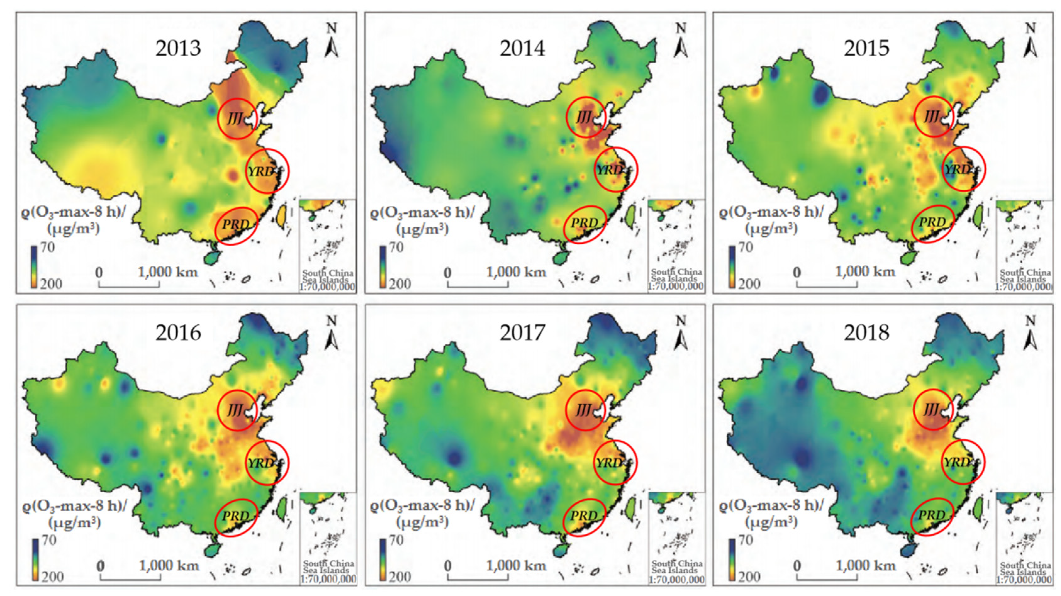
3. Spatiotemporal Distribution of Tropospheric Ozone in China

Tropospheric O₃ exhibits different characteristics in different regions. Understanding the spatiotemporal characteristics of O₃ concentration is essential for controlling atmospheric O₃ pollution. Since 2012, the Chinese government has included atmospheric O₃ as a regular pollutant monitoring indicator, and the national monitoring network has brought convenience to the study of the spatial and temporal characteristics of atmospheric O₃.

Most of Chinese population lives in the east of China, especially in the three most developed regions of Jing-Jin-Ji (JJJ, including Beijing, Tianjin, and Hebei province), Yangtze River Delta (YRD, including Shanghai, Zhejiang, Jiangsu, and Anhui provinces), and Pearl River Delta (PRD, including nine cities in south-central of Guangdong province). These regions are also the areas with the highest emissions of anthropogenic NOx and VOCs, thus leading to serious regional atmospheric ozone pollution. Therefore, these regions are the key areas for preventing and controlling air pollution. Figure 1 shows the spatial distribution of annual average O₃-max-8 h in China from 2013 to 2018 [19]. The overall O₃ concentration presented a spatial distribution pattern of higher in the east and lower in the west. The high-value areas of O₃-max-8 h were mainly concentrated in the North China Plain in the east, such as Hebei province and Shandong province, where O₃-max-8 h was higher than 180 μg·m⁻³; followed by the Yangtze River Delta and its nearby areas with an O₃-max-8 h ranging from 120 to 160 μg·m⁻³. The O₃-max-8 h in the southern Pearl River Delta region was also in the range of 120 to 160 μg·m⁻³, but the high-value area was smaller than the Yangtze River Delta area. The O₃-max-8 h was lower in the western region, ranging from 70 to 100 μg·m⁻³, and reaching as low as 62 μg·m⁻³ in the Hami area. The spatial distribution of O₃-max-8 h was consistent with the distribution pattern of its precursor emissions. The NOx emission intensity was higher in the east than that in the west, with the highest values distributing in the Beijing–Tianjin–Hebei region, Yangtze River Delta and Pearl River Delta. From 2013 to 2018, the 90th percentile of O₃-max-8 h concentration in China gradually increased with an annual growth rate of 2.6 μg·m⁻³ per year. The highest O₃-max-8 h (≥180 μg·m⁻³) zone mainly occurred in the North China and Yangtze River Plains, which gradually expanded in the North China Plain (NCP) while shrinking in the YRD and PRD.

Based on the data of ozone monitoring instruments (OMI) from 2005 to 2014, the tropospheric ozone trend in mid-eastern China (including 10 major cities) was studied [20]. The results showed that the mixing ratios of tropospheric ozone column were fairly stable, but those of ground-level clearly increased, by 12.38%. The concentration of ground-level ozone reached the maximum value from May to June, while the minimum value was from November to December. The concentrations of ground-level ozone increased with the cumulative increments of 6.3, 6.6, and 10.2 ppbv (parts per billion by volume) in Beijing, Shijiazhuang and Tianjin, respectively, from 2005 to 2014. Additionally, the concentration of ground-level ozone increased rapidly in Tianjin during 2012-2014, showing an increase of 13.25% compared with 2010–2011, which might be due to the more rubber and chemical companies around Tianjin. In contrast, the concentration of ground-surface O₃ in the Beijing area showed a slower rising trend from 2005 to 2014. According to previous studies, atmospheric O₃ pollution often appeared in the region of Beijing–Tianjin–Hebei, among which Beijing and Baoding were more polluted [21,22].

The temporal and spatial distribution characteristics of atmospheric O₃ in the Beijing–Tianjin–Hebei region during 2013–2015 indicated that O₃ concentration presented obvious seasonal variation, with the highest concentration in late spring and summer, and showed a single peak distribution during daytime, with the maximum value appearing around 15:00. In contrast, the concentration was lower and had little fluctuation throughout the day in autumn and winter. The higher values of O₃-max-8 h were mainly distributed in north-central Beijing, Chengde and Hengshui [23]. The seasonal variations of tropospheric O₃ concentration distribution in Beijing, Shanghai, Guangzhou and Chengdu were similar, with the highest value generally occurring in summer and the lowest value generally appearing in winter [24].

Table 2. Summary of tropospheric ozone concentrations in some regions of China.

Region	Period	Maximum Value or Range (ppbv)	Precursors	Reference
Jing-Jin-Ji Urban Agglomeration	2013–2015	(O3-8 h) 77.5–81 *		[23]
Jing-Jin-Ji region	January–December 2017	(O3-1 h) 139.5		[22]
$\mathrm{Chang} \mathrm{Ping}, \mathrm{Beijing}$	21 June–31 July 2005	(O3-1 h) 286	VOCs (Alkenes, aromatics)	[25]
Beijing	2014–2017	(O3-8 h) 98–103 *		[24]
Nantong, Jiangsu	2013–2015	(O3-8 h) 83.5 *	CO, VOCs (propene, ethane, xylene, acetylene)	[26]
$\mathrm{Taicang}, \mathrm{Shanghai}$	4 May–1 June 2005	(O3-1 h) 127	VOCs (Alkenes, aromatics)	[25]
Shanghai	2014–2017	(O3-8 h) 76–94 *		[24]
Jiaxing, Zhejiang	27 June–31 August 2013	(O3-1 h) 84 *	CO, NO2	[27]
Shouxian, Anhui	January 2015–December 2018	(Monthly mean) 51.3		[28]
Wan Qing $\mathrm{Sha}, \mathrm{Guangzhou}$	20 April–26 May 2004	(O3-1 h) 178	VOCs (aromatics)	[25]
Guangzhou	2014–2017	(O3-8 h) 76–85 *		[24]
$\mathrm{Renshoushan} \mathrm{Park}, \mathrm{Lanzhou}$	19 June–16 July 2006	(O3-1 h) 143	VOCs (alkenes)	[25]
$\mathrm{Shenyang}, \mathrm{Liaoning}$	2013–2015	(O3-8 h) 77 *	NO2, CO	[29]
Jiangxi	January 2015–August 2017	(O3-1 h) 40.5–70 *		[30]
Chengdu, Sichuan	January 2014–December 2016	(O3-8 h) 2.5–146.5 *		[31]
Chengdu	2014–2017	(O3-8 h) 68–94 *		[24]
Sichuan	July 2017	(O3-8 h) 141.3 *	VOCs	[32]
NCP	June 2017	(O3-1 h) 91 *		[33]

1. O₃-1 h: Maximum 1 h average; O₃-8 h: Maximum 8 h average. 2. Note: * For rough estimates from the literature.

summarizes the tropospheric ozone concentrations in some regions of China.

The summer–winter differences are due to the general meteorological conditions including the variability of irradiation levels affecting free-tropospheric and boundary-layer photochemistry, which is also one of the main sources of the high background O₃ on the surface [9]. From 2013 to 2019, the weather in the North China Plain (NCP) drove an increase in surface O₃ [34]. The hot weather in the NCP in summer is usually driven by a wide range of anticyclone conditions, which is regarded as a typical climate pattern for the number of days of O₃ pollution [33]. The influence of the boundary layer on ozone in the summer afternoon cannot be ignored. Under the conditions of free convection, the stronger the ultraviolet radiation (UV), the higher the temperature, the lower the relative humidity (RH) and the higher the boundary-layer height (BLH), the more serious the ozone pollution was in Shijiazhuang in summer of 2018–2019 [35]. The increase in radiation during the day may cause the boundary layer to rise, and the accumulated O₃ may mix down to the boundary layer, affecting the near-surface ozone concentration. The history of the air mass is an important factor in determining the magnitude and potential signs of the impact of entrainment on surface O₃ through atmospheric boundary-layer growth [36]. As the height of the boundary layer increases, the O₃ in the residual layer (RL) is transported to the boundary layer. Some studies have found that the mixed ozone from the RL contributes 50–70% of the maximum concentration near the surface for the next day, and the rest comes from chemical production and possible advection [37,38].

Based on the tropospheric O₃ concentration data of 16 urban monitoring stations from June 2013 to May 2014, the spatiotemporal distribution characteristics of atmospheric O₃ in the Yangtze River Delta region were studied [27]. The results showed that the annual average O₃ concentration was higher in the cities near the sea and lower in the cities that are inland. The concentration of atmospheric O₃ showed a seasonal variation, with higher concentration in summer and lower concentration in winter. The higher O₃ pollution area was located in the north of Hangzhou Bay in summer, while the higher O₃ pollution area was located in the eastern coastal zone in winter. The diurnal variation of O₃ concentration in the Yangtze River Delta was unimodal throughout the four seasons. The daily minimum O₃ concentration appeared around 06:00 in summer, and was delayed by about one hour in the other seasons, and the daily maximum O₃ concentration appeared around 15:00 in all seasons. Based on the OMI data, the spatiotemporal distribution of the tropospheric O₃ in the Yangtze River Delta region showed a significant zonal difference, increasing with latitude [39]. According to the monitoring data of 72 state-controlled stations in Jiangsu province from 2013 to 2015, the spatiotemporal distribution characteristics of tropospheric O₃ were studied [26]. The results indicated that the annual mean value of atmospheric O₃ in Jiangsu province showed a significant spatial difference, with the concentration gradually decreasing from coast to inland. Tropospheric O₃ showed the highest concentration in Yancheng city, while it was lower in Changzhou, eastern Wuxi and Xuzhou cities. The 90th percentile concentrations of O₃-8 h were significantly different from north to south. The atmospheric O₃ concentration was relatively higher in the cities of Nanjing, Yangzhou and Zhenjiang, while the lower concentrations were found in the cities of Xuzhou and Suqian. It was reported that the atmospheric O₃ peak occurred in the afternoon in Shanghai from 2006 to 2016 [2]. The areas with O₃ concentration exceeding the limit of Chinese national ambient air quality standards were mainly in the southwest suburbs of Shanghai, and the atmospheric O₃ concentration decreased from the southwest suburb to the northeast urban areas. It was reported that the tropospheric O₃ pollution in the Yangtze River Delta region was more serious in Shanghai, Ningbo and other cities [28]. It should be noted that the concentrations of near-ground-surface O₃ in Shanghai, Hangzhou, Hefei and Nanjing in the Yangtze River Delta region have increased slightly during the past 10 years (from 2005 to 2014), but the increase degree was smaller than that in the Beijing–Tianjin–Hebei region. The distribution of atmospheric O₃ pollution in the Yangtze River Delta showed relatively obvious flaky distribution characteristics, and the higher emissions from motor vehicles in the Yangtze River Delta urban cities were the main sources of atmospheric O₃ in this region [20].

The average near-ground-surface O₃ concentration in the Pearl River Delta region was slightly lower than those in the Beijing–Tianjin–Hebei region and the Yangtze River Delta region during 2013–2018 [19]. The characteristics of atmospheric O₃ pollution in the Pearl River Delta region and Guangdong province were reported based on the large-scale and long-term continuous O₃ monitoring data of recent years [40]. The results showed that the atmospheric O₃ concentration in the Pearl River Delta region was higher than that in the northwest of Guangdong province. Outside of the Pearl River Delta region, the eastern area of Guangdong province has the highest atmospheric O₃ level. The O₃ concentration was higher in the central southern part of the Pearl River Delta and the eastern part of Guangdong, while it was lower in the west. The concentration of atmospheric O₃ was higher in summer and autumn, and lower in winter and spring. Due to the large differences of the climate between the Pearl River Delta region and the Beijing–Tianjin–Hebei region and the Yangtze River Delta region, the better atmospheric diffusion conditions made it difficult for atmospheric O₃ to accumulate in the Pearl River Delta region.

In addition to the regions of Beijing–Tianjin–Hebei, the Yangtze River Delta and the Pearl River Delta, other regions in China have also been conducted research on local atmospheric O₃ pollution. The spatial and temporal distribution of atmospheric O₃ pollution in the Bohai Rim region of Liaoning province was reported [41]. The results showed that the atmospheric O₃ pollution presented obvious seasonal variation characteristics, and the main months in which the O₃ concentration exceeded the limit of Chinese national ambient air quality standards were from May to August. The diurnal variation of atmospheric O₃ was unimodal, and the peak concentration appeared in the afternoon. The higher O₃ concentration areas were mainly located in Yingkou in the central Bohai Sea Economic Rim of Liaoning, while the O₃ level was relatively lower in Dalian and Huludao. The investigation of atmospheric O₃ pollution in Shenyang area from 2013 to 2015 showed that the concentration of O₃ in the periphery of the city was higher than that in the center of the city [29]. Compared with the periphery of the city, the concentration of NO emissions is higher in urban centers. The increase in NO emissions leads to an increase in the titration of O₃, which inhibits the accumulation of O₃. The variation of O₃ concentration showed obvious seasonal characteristics, with the highest being in summer and the lowest in winter. The diurnal variation showed a unimodal distribution, with the trough value at 06:00 and the peak value at 14:00. Over continental sites, important nocturnal ozone destruction is observed due to dry deposition and NO titration [42]. The tropospheric O₃ concentrations showed significant “weekend effects”, with higher O₃ concentrations in weekends than in weekdays during the daytime while little difference at night. The spatiotemporal distribution characteristics of surface O₃ concentrations in Fujian province in 2016 was studied [43]. The results showed that the O₃ concentration was higher in spring and autumn, whereas it was lower in winter. The O₃ concentrations in the coastal cities were higher than those in the inland cities. The monthly changes in O₃ concentration presented a bimodal pattern, with peaks generally appearing in May and September. The diurnal variation curve of O₃ concentration was a single peak, which usually appeared at about 14:00. The spatiotemporal distribution characteristics of the atmospheric O₃ concentrations in Jiangxi province during 2015–2017 showed that the higher values of atmospheric O₃ were mainly distributed in the northeast areas such as Nanchang city and Jiujiang city, while the lower values were mainly distributed in the western areas such as Xinyu city and Yichun city [30]. The monthly variation of atmospheric O₃ concentration showed a double-peak pattern with higher values in May and September, while the daily variation showed a single-peak pattern with higher values at 14:00–16:00. The temporal characteristics of atmospheric O₃ pollution and the meteorological factors in Chengdu during 2014–2016 were reported, and the results showed that the situation of atmospheric O₃ pollution in Chengdu became worse in recent years [31]. The concentrations of atmospheric O₃ showed obvious seasonal variation characteristics—higher in summer and spring, while lower in winter and autumn. The diurnal variation of O₃ concentration showed a unimodal distribution, with the peak appearing at around 15:00, which was consistent with the diurnal variation of air temperature and solar irradiance. The distribution of surface O₃ in Chongqing city in 2018 showed that the O₃ concentration in spring to autumn exceeded the limit of Chinese national ambient air quality standards [44]. It was pointed out that the concentration of atmospheric O₃ was the highest and the pollution lasted for a long time in summer. Severe O₃ pollution in the Sichuan basin in summer was also reported [32].

For most urban stations, the potential ozone (Ox = O₃ + NO₂) is a conservative amount over a short time scale. When the freshly emitted NO reacts with O₃, NO₂ is formed in a few minutes, so some local NO₂ in the troposphere is produced at the expense of O₃ [45,46]. Generally, the surface ozone production is controlled by NOx. The diurnal patterns of O₃ and nitrogen dioxide were opposite in Chengdu, indicating that the O₃ sensitivity was VOC-limited [32]. The relationship between atmospheric O₃ with non-methane hydrocarbons (NMHCs) and NOx in Guangzhou in 2011 was discussed, and the results showed that controlling highly reactive NMHCs and NOx could effectively reduce O₃ concentration [47]. It should be noted that the reduction in NOx may have positive or negative impact on local ozone production. Ozone sensitivity was different at different stages, and reducing NOx emissions had a negative impact on Shenzhen’s ozone pollution control from 2015 to 2018 [48].

4. Relationship between Tropospheric Ozone and Its Precursors

As mentioned before, tropospheric O₃ can be produced by photochemical reactions of VOCs, NOx and other primary pollutants under solar radiation. Theoretically, the content of O₃ in the troposphere can be controlled by controlling the emission of VOCs and NOx. However, the execution difficulty is that the relationship between the generation of O₃ with VOCs and NOx is nonlinear. An investigation into the relationship between the atmospheric O₃ with NOx and VOCs showed that the formation of O₃ depended on NOx in rural areas, while it depended on both NOx and VOCs in urban areas [49]. A study on the formation of tropospheric O₃ and the effect of VOCs in Shanghai found that alkanes and aromatic hydrocarbons were the dominant VOCs, and aromatic hydrocarbons contributed most to the chemical production of atmospheric O₃ [50]. Similar results were found in Guangzhou, where aromatics accounted for 70% of the atmospheric O₃ formation potential (OFP) [51].

A numerical simulation control of atmospheric O₃ pollution was carried out in Shenzhen city based on the two-dimensional air-quality model [52]. The results showed that the generation of atmospheric O₃ was the product of the interaction between NOx and VOCs, and the emission of VOCs was more important. The co-emission reduction in the precursors might effectively reduce the atmospheric O₃ pollution. As one of the major species of VOCs emitted from biogenic sources, isoprene is highly reactive and plays an important role in the generation of oxidants for a range of photochemical reactions. A study on the contribution of isoprene emissions to the ground-level O₃ formation in Beijing showed that isoprene emissions accounted for almost half (49.5%) of OFP at 13:00 in August of 2010, suggesting that isoprene played an important role in the ozone formation [53]. According to the results of field sampling, the most influential substances related to OFP in Zhengzhou urban area were ethanol, 2-hexanone, o-trimethylbenzene, and the industrial VOCs were a source of O₃ pollution in Zhengzhou [54]. It is reported that fire can affect NOx, CO and VOCs, which will significantly affect the background value of O₃ [55].

Therefore, the prevention and control of atmospheric O₃ pollution cannot be simply through a programmed control of primary pollutants. The influence of VOCs and NOx on atmospheric O₃ production can be characterized by a VOCs-sensitive zone and NOx-sensitive zone [56]. In general, the oxidation of VOCs with high concentrations of VOCs can produce higher concentrations of RO₂·, and the emission of NO can lead to reaction R4 enhancement. Therefore, the amount of O₃ production increases with the increase in NOx, and this type of O₃ generation mechanism is described as the NOx-sensitive (limiting) type. When the concentration of NOx is high and the concentration of VOCs is low, the reaction rate of NO + O₃ is faster than that of NO + RO₂·. In this case, the cumulative amount of O₃ may decrease with the increase in NOx, and may increase with the increase in VOCs, hence this mechanism is described as VOC-sensitive (limiting) or NOx saturation. When the generation of O₃ is restricted by VOCs, the O₃ generation can be controlled by reducing the emission of VOCs. Similarly, when the formation mechanism of O₃ is NOx-limiting type, the O₃ content can be controlled by reducing the emission of NOx. The sensitivity of summer O₃ in Beijing during 2010–2015 was studied [57]. The results showed that when VOCs/NOx was 2.0, the urban areas were more sensitive to VOCs and high concentrations of VOCs persisted in western and northern rural areas. When VOCs/NOx was 3.0~5.0, O₃ precursors aged, and lower VOCs concentrations appeared in the northern and southern suburbs. A comprehensive investigation into O₃ and its precursors and low tropospheric aerosols over a survey site located at the University of Chinese Academy of Sciences in Beijing showed that the photochemical generation of O₃ in the boundary layer was restricted by VOCs in hazy weather, while the photochemical reaction of O₃ became VOCs–NOx-limiting in the clean weather [58]. According to the sensitivity analysis, the atmospheric O₃ generation was largely determined by VOCs when air masses came from the polluted areas in the south. Therefore, reducing VOCs emissions from the industrial areas and urbanized areas could help to reduce the ozone pollution at this site.

Currently, there are a variety of methods that can be used to study the sensitivity of atmospheric ozone generation. Some commonly used methods are as follows.

(1)

Ozone production efficiency (OPE, defined as the number of ozone molecules produced for each NOx molecule oxidized). A lower OPE value (<4) indicates that the free radical cycling efficiency is lower, so VOCs are the limiting factor, and the formation of O₃ is controlled by VOCs. Conversely, a higher OPE value (>7) indicates that the free radical cycling is efficient and the formation of O₃ is limited by NOx. When the OPE value is medium (4–7), O₃ generation is controlled by both VOCs and NOx. The OPE values in rural and suburban areas of Beijing were measured during the 2008 Olympics [59]. The results showed that higher OPE values corresponded to NOx limiting under low NOx conditions, whereas OPE values were lower under high NOx conditions.

(2)

Relative incremental reactivity (RIR, defined as the ratio of the decrease in O3 production rate to a given reduction in the precursor concentration) is a measure of the sensitivity of a single precursor. Cardelino et al. [60] first used a scenario test calculated by a box model to simulate the response of ozone to changes in precursors. The calculation result can be expressed by the following formula.

$$\mathrm{RIR}\left(\mathrm{X}\right)=\frac{\Delta {\mathrm{O}}_3\left(\mathrm{X}\right)/{\mathrm{O}}_3}{\Delta \mathrm{C}\left(\mathrm{X}\right)/\mathrm{C}\left(\mathrm{X}\right)}$$

where X represents a group of major pollutants, and O₃ represents the modelled O₃ concentration. ΔC(X)/C(X) gives the relative change in the primary pollutants in one of the sensitivity tests, and the relative change in modelled ozone concentration is given by ΔO₃(X)/O ₃. In the study on atmospheric ozone pollution conducted in Chengdu in September 2016, the anthropogenic variation of the main pollutant in the sensitivity test was chosen as 20% in the RIR analysis, because when the variation value was greater than 20%, the RIR value deviated due to the significant change in the simulated free radical concentration [61]. The RIR results demonstrated that anthropogenic VOCs reduction is the most efficient way to mitigate ozone pollution, of which alkenes dominated more than 50% of the ozone production [61].

(3)

H₂O₂/HNO₃ ratio method. A ratio of 0.8–1.2 is used to separate NOx-sensitive and VOC-sensitive regions. If the ratio is small, it can be considered as a sensitive area of VOCs, otherwise it is a sensitive area of NOx. Based on this method, the urban areas were sensitive to VOCs while the rural areas were sensitive to NOx in Hong Kong [62].

(4)

Empirical kinetic modelling approach (EKMA). The EKMA model can give the isoline of O₃ maxima under different NOx and VOCs due to photochemical reactions. The initial design was to simulate the maximum O₃ concentrations under different precursor emission scenarios to develop O₃-polluting precursor emission mitigation strategies [48]. The EKMA diagram illustrates the sensitivity of O₃ to VOCs and NOx and how the ratio of VOCs/NOx affects the production of O₃. The ridge line of the EKMA curve is formed by connecting the convex points of each curve. EKMA is divided into two parts: when the VOCs/NOx ratio is located in the left of the ridge line, the O₃ formation is limited by VOCs, otherwise the O₃ formation is limited by NOx [63]. The advantages of the EKMA curve method are as follows: Firstly, it can provide both a qualitative and quantitative basis for O₃ prevention and control; Secondly, it is a link between secondary and primary pollutants, which can better express the relationship between the two types of pollutants; Thirdly, the shape of EKMA will change under different conditions, which can better reflect the specific local conditions. For example, a Chinese EKMA was developed by following the traditional approach of constructing EKMA curves to explore the cost-effective emission reduction strategies for both O₃ and PM_2.5, suggesting that a strategy of “focusing on VOCs first, then NOx” could be effective in controlling PM_2.5 and O₃ pollution mitigation in the long term [64].

According to current research on atmospheric ozone formation regimes, most of the urban areas in China are in VOCs-limited zones, with anthropogenic VOCs (especially reactive aromatics and alkenes) playing a dominant role. However, some variations were found in the chemistry regime of atmospheric ozone formation in different regions.

5. Factors Affecting Atmospheric Ozone Level

5.1. Precursors

Photochemical reactions are the main source of tropospheric O₃, whose concentration is closely related to the concentrations of NO_X and VOCs. Generally, the ozone concentration in urban and suburban areas is mainly affected by photochemistry. The transmission of the “aging” urban plume has resulted in extremely high O₃ levels (up to 286 ppbv) in rural sites downwind of Beijing, which are most affected by local photochemistry. In the suburbs of Shanghai, Guangzhou, and Lanzhou, strong in situ photochemical production is the main focus [25]. The characteristics of VOCs pollution and its contribution to atmospheric O₃ formation in Wuhan city was studied [65]. The results showed that the local pollution source was the main source of VOCs pollution, and olefins had the highest chemical activity and the biggest contribution to atmospheric O₃. Based on the observed data of atmospheric O₃ and its precursors in Beijing in autumn 2004, the O₃ generation efficiency in the region near the main traffic lines was calculated, and the results suggested that the reduction in VOCs emission was beneficial to the reduction in atmospheric O₃ concentration [66]. Carbonyl compounds are important members of the VOCs family and are important precursors of secondary organic aerosols (SOA); alkenes, aromatics, and isoprene are primarily secondary products of carbonyl compounds; carbonyl groups are usually dominant in the formation of atmospheric O₃ in rural areas [67]. Biovolatile organic compounds (BVOCs) played an important role in the formation of tropospheric O₃, especially in urban areas [68]. The effects of BVOCs emission on the formation of tropospheric O₃ and SOA were studied by using a WRF-CMAQ simulation system, and the results showed that the biogenic emission peaked in summer and decreased gradually from south China to north China [69]. High BVOCs emissions in eastern and southwestern China increased the ground-level ozone, particularly in the Beijing–Tianjin–Hebei region, Sichuan Basin, Yangtze River Delta and the central Pearl River Delta. The ozone isolines in the summer of 2013 showed that the O₃ concentrations were controlled by NOx in most areas of China, and the effect of VOCs reduction on O₃ concentration was less, except in the urban areas of Shanghai and Guangzhou [70]. An investigation into the O₃ exposure indices and the source contributions in the forests of China throughout the entire year of 2013 suggested that the O₃ production was much more due to NOx than due to VOCs [71].

5.2. Meteorological Factors

Tropospheric O₃ concentration was found to be positively correlated with ambient air temperature, and negatively correlated with wind speed and relative humidity. On the contrary, NOx was positively correlated with relative humidity, and negatively correlated with temperature [72]. Under normal conditions, temperature can affect the concentration of O₃ by influencing the reaction rate, while wind speed can affect the dilution and diffusion of pollutants. Relative humidity has some influence on photochemical reaction processes, and higher relative humidity can cause wet deposition and even lead to the erosion of pollutants by rainwater. It was reported that aerosol could change the photolysis rate of trace gases [73]. Absorption of aerosols can reduce UV flux throughout the troposphere, resulting in a reduction in near-surface O₃. Based on the analysis of the meteorological effect on atmospheric O₃ in Tianjin from 2009 to 2015, it was concluded that the tropospheric O₃ level was more dependent on temperature in the afternoon than in the morning since the daily maximum temperature usually occurred in the afternoon [74]. In spring and summer, the maximum daily O₃ was less dependent on the solar radiation than the ambient temperature. In autumn and winter, solar radiation played a more important role in determining O₃ level. The concentration of atmospheric O₃ had a weak negative correlation with the wind speed in spring, summer, and autumn, but a weak positive correlation with the wind speed in winter. Moisture in spring and autumn also had an effect on atmospheric O₃ concentration due to the compensation between water vapor and O₃. Air with high humidity raised ·OH radicals and produced higher O₃ concentration in the areas with high NOx. At the same time, a rise in water vapor also consumed excited oxygen atoms and increased the loss of O₃. The relationship between heat waves and the concentration of atmospheric O₃ in the Yangtze River Delta was discussed [75]. The results showed that under the action of heat waves, the water vapor content and the cloud cover of the Yangtze River Delta were reduced because of the anticyclone controlled by the downdraft, which increased the concentration of atmospheric O₃ in the presence of intense solar radiation. In the case of climate warming, the chemical reaction may cause the atmospheric O₃ content to increase significantly, and the high temperature can also promote vertical turbulence and horizontal advection to some extent, which is beneficial to the removal of O₃, but the extent is much less than that of the chemical action. Relevant studies have shown that the heat-island effect was directly or indirectly related to the increase in the emission of atmospheric O₃ and its precursors. The pollution of atmospheric O₃ in the Yangtze River Delta is becoming more and more serious, and the heat-island effect is the key factor affecting the atmospheric O₃ level. There was a positive correlation between heat-island effect and the atmospheric O₃ concentration in the Yangtze River Delta. The factors influencing the urban heat-island effect and atmospheric O₃ include landscape, topography and population, but land surface temperature and vegetation index are the most important [76]. It was reported that the structure and evolution of weather was of great significance to the atmospheric photochemical pollution [77]. The level of ozone concentration affected by the surface and the boundary layer depends on the main weather conditions that are conducive to large-scale subsidence [78]. The eastern and central basins of the Mediterranean have obvious top-down ozone deposition, which is caused by adiabatic convection over the Persian Gulf during the Indian monsoon season [79]. The influence of Asian continental outflow on the regional background ozone level in the northern South China Sea was studied, and the results indicated that the Asian continental outflows brought about by the winter monsoon could be immense, and intense enough to affect regions from far south, at latitudes similar to Antarctica [80].

5.3. Atmospheric Particulates

Aerosols are small particles suspended in the atmosphere and play an important role in the earth’s radiation balance, air quality and cloud microphysics. They directly affect the regional and global climate by absorbing and scattering solar and terrestrial radiation, and indirectly affect the global climate by altering cloud formation characteristics. Ambient aerosol particles are mainly derived from anthropogenic activities and natural sources, such as residential heating, automobile exhausts, open-air combustion and volcanic activities [81]. The Asian monsoon brought in aerosols from biomass burning in southeast Asia, which were mixed with moist air particles in southern China, eventually reaching high aerosol concentrations in the spring, which reached the lowest concentration in winter [82]. There was a significant negative correlation between O₃ and particulate matter in the margin of Tarim Basin, indicating that the effect of dust on solar transmittance in the atmosphere lead to a decrease in net O₃ productivity [83]. The concentration of O₃ was influenced by the nonuniform chemical processes occurring on the surface of particles, so increasing the concentration of PM_2.5 could weaken the atmospheric radiation. This would allow the O₃ level to be suppressed by eliminating ultraviolet light, which was consistent with the conclusions of Wang et al. [22] and Qu et al. [84]. In 2017, 338 main cities in China were selected to sample ambient air for 365 days to compare the concentrations of O₃, NO₂, SO₂, particulate matter and CO in the atmosphere [85]. The results showed that O₃ concentrations were significantly correlated with PM₁₀ in 238 cities, among which, the coefficients in 142 cities were positive whereas those in 96 cities were negative. Most cities with positive correlations were mainly located in the south and northeast, while most cities with negative correlations were mainly located in the north of China. There was no significant correlation between O₃ concentration and PM₁₀ concentration in 100 cities. O₃ concentrations were significantly correlated with PM_2.5 in 250 cities, among which, the coefficients in 117 cities were positive and those in 133 cities were negative. Most cities with positive correlations were mainly located in the south, while most cities with negative correlations were mainly located in the north. There was no significant correlation between O₃ concentration and PM_2.5 concentration in 88 cities. The possible reason for the above results was that NOx and VOCs would simultaneously increase significantly on the particulate matter (PM) pollution days in many cities, and the increase in these precursors influences the atmospheric O₃ concentration more than the particulates. Atmospheric O₃ was usually used as a tracer for photochemical reactions. A large amount of O₃ was used as an oxidant to enrich the secondary components of PM_2.5 through a secondary photochemical process, so higher PM_2.5/PM₁₀ usually indicated the existence of more active photochemical reactions. To some extent, PM_2.5/PM₁₀ could be used as a reference index for the types of air pollution, that is, higher or lower PM_2.5/PM₁₀ indicated the complicated pollution types related to photochemical reaction [86].

The main fixed sources of PM_2.5 and PM₁₀ are smoke and dust produced by fuel combustion and gas oil during heating in industrial enterprises, such as power generation, oil and printing. The main moving source is exhaust gas emitted by road traffic vehicles into the atmosphere. The temporal characteristics of PM_2.5 in Anhui province showed that PM_2.5 decreased from January to July, and increased from July to December, that is, the concentrations of PM_2.5 were lower in summer and higher in winter [87]. Some studies showed that PM_2.5 and PM₁₀ were positively correlated with NO₂ and CO, and weakly correlated with O₃. The high concentration of O₃ in highly oxidized air in high-temperature seasons promoted the formation of secondary particulate matter, which made PM_2.5 positively correlated with O₃ [88]. Several studies have found that reducing PM_2.5 might lead to an increase in atmospheric O₃, and reducing emissions of NOx and VOCs is required to overcome this effect. A more important factor affecting O₃ trends in the North China Plain (NCP) from 2013 to 2017 was the reduction in PM_2.5, which slowed down the sink of hydroperoxy radicals, thus speeding up O₃ production [89]. In addition, atmospheric particles could directly affect the scattering and absorption of radiation, consequently changing the intensity of incident ultraviolet radiation, and affecting the production of O₃. The formation of O₃ decreased with the decrease in UV radiation or light scattering associated with PM_2.5 [90].

5.4. Weekend Effect

The weekend effect refers to the phenomenon of different atmospheric pollutants concentration between weekends and weekdays, mainly caused by human activities. On weekdays, the main anthropogenic precursor emissions are due to commuting driving, especially during the day. However, on the weekends, the main anthropogenic precursors might come from family-related recreational activities. The difference in vehicle emissions between weekdays and weekends is mainly related to fuel combustion products, fuel consumption, and the traffic patterns of gasoline and diesel vehicles. Heavy-duty diesel vehicles are the main source of NOx and black carbon (BC), while light-duty gasoline vehicles are the main source of CO₂. In general, the diesel-fueled vehicles showed a significant reduction during weekends, resulting in a significant reduction in NOx and BC emissions. If the atmospheric system was at nitrogen oxide saturation in urban areas, the reduction in NOx emission on weekends may lead to a reduction in O₃ titrations, which can reduce the inhibition of O₃ formation, resulting in an increased O₃ concentration on weekends. The “ozone quenching hypothesis” and “NOx reduction hypothesis” in the weekend effect prove that NOx plays a complex role in ozone production and termination [16]. The concentration of atmospheric O₃ increased from weekdays to weekends for a number of sites in the Northern Front Range metropolitan area (NFRMA) of Colorado, with weekend reductions in NO₂ at two sites in downtown Denver between 2000 and 2015, indicating that the region was in a NOx-saturated ozone production regime [91]. Similar results were found in Shenyang city from 2013 to 2015 [29]. Koo et al. [92] investigated the weekend effect in the Midwest (north-central and northeast) of the United States in the summer of 2005, and the results showed that the reduction in O₃ on weekends depends on the increase in NOx emissions leading to an increase in O₃ titration. The investigation of the weekend effect on O₃ in Beijing in 2014 showed that the O₃ concentration at weekends was overall higher than that on weekdays, especially in urban centers [93]. The atmospheric O₃ generation might be limited by VOCs during summer, autumn and winter. However, the weekend O₃ concentration was lower than on the working days in spring, suggesting that O₃ production might be limited by NOx in this season. On the urban scale, the weekend effect in the central area of the city was larger than that in the suburb, but on the local scale, the weekend effect showed a downward trend, with an increase in urbanization. Weekend O₃ changes depend on the intensity of the sunshine and the ratio of VOCs to NOx emissions [94].

6. Prevention and Control Measures for Tropospheric Ozone Pollution

In a particular region, the level of tropospheric O₃ depends on meteorology and the interaction between O₃ precursors. The distinction of these impacts is important for evaluating the effectiveness of past emission reduction measures and clarifying the direction of future control plans [95]. In order to effectively reduce the tropospheric O₃ pollution, it is necessary to strengthen the prevention and control of corresponding pollutants.

(1)

The technology and energy structures should be improved, and the emissions of NOx and highly reactive VOCs should be controlled. Pollution can be reduced by closing high-polluting factories, setting up coal-free zones, restricting vehicles, installing tailpipe cleaners and promoting the use of “three-way” catalytic converters. In addition, improving the fuel, changing the composition of gasoline, or using alternative fuels can reduce the pollution of tail gas.

(2)

The monitoring and management should be strengthened. Measures should be taken to avoid the occurrence of photochemical smog by using warnings issued from monitoring equipment. When oxidant concentrations reach dangerous levels, authorities should prohibit garbage incineration, reduce road vehicles or shut down some factories temporarily. Emissions from oil refineries, petrochemical plants and nitrogen fertilizer plants should be severely restricted by regulations. The VOCs from landfills have been reported to contribute to the formation of O3 and photochemical smog [96]. Therefore, there is a need for integrated waste management policies, including source reduction and waste recovery, to reduce VOCs emissions.

(3)

The prevention and control of VOCs and NOx pollution should be strengthened. The control measures should focus on the industries with relatively serious pollution, such as petrochemicals and printing. The comprehensive treatments for the waste gas produced by these processes should be strengthened. The waste-gas-containing pollutants should be centralized processing, and the treated tail gas should be recycled. The use of raw and auxiliary materials with low VOCs content and low reactivity should be promoted, and the production processes should be optimized as much as possible. The implementation of urban forest measures for O3 should be undertaken in noncompliant areas, that is, the gradual replacement of high-BVOC-emission species with low-emission species, which can effectively control the emission of VOCs to reduce O3 production [97]. Some regions have been effective in curbing O3 pollution through synergistic control of VOCs and NOx, but O3 remains a problem in most places, especially in areas with high ozone pollution such as Beijing–Tianjin–Hebei, the Yangtze River Delta and the Pearl River Delta. Xiang et al. [64] pointed out that equally reducing NOx and VOCs emissions in the initial stage may have the least benefit for air pollution improvement in Beijing–Tianjin–Hebei and the surrounding areas because the NOx-focused strategies may exacerbate O3 pollution. Emission reduction programs should be optimized in conjunction with short-term or long-term targets to control VOCs and NOx emissions more scientifically.

(4)

O3 pollution should be controlled in coordination with PM2.5/PM10. O3 and PM2.5 co-pollution conditions occur under meteorological conditions of high relative humidity, high surface air temperature and low wind speed [98]. When PM2.5 and O3 interact under different ambient meteorological conditions, it depends on the dominant party. Tropospheric O3 and particulate matter interact through aerosol formation, nonhomogeneous reactions on the surface of the particulate matter and changes in the aerosol-induced photolysis rate. The relationship between PM2.5/PM10 and the atmospheric ozone is therefore complex. High PM2.5/PM10 concentrations can affect the aerosol radiative effects and the surface inhomogeneous reactions, which are also influenced by different regions and meteorology, with long-range transport of air masses bringing about cross-regional pollution of PM2.5 and O3 [99]. Long-term mitigation of PM2.5 and O3 pollution control should be addressed by optimizing the zoning of prevention and control areas and implementing local and targeted measures. Predictive simulation models and representative regional monitoring networks should be developed, and synergistic mitigation strategies for PM2.5 and O3 pollution should be explored. The effective synergistic control measures remain a difficult area for future research.

7. Summary and Recommendations

High ozone concentrations are harmful to humans and the ecological environment, and atmospheric ozone pollution is becoming a major environmental problem that has been plaguing the economic development in China. There are significant regional differences in the distribution of O₃-max-8 h in China. The overall level of O₃-max-8 h in the NCP is higher than that of other regions. Due to economic development and dense population, the eastern region has a higher level of O₃-max-8 h, and the high-value areas are distributed in flakes and bands. The high O₃-max-8 h areas are mainly concentrated in the Beijing–Tianjin–Hebei region, the Yangtze River Delta and the Pearl River Delta. In general, the tropospheric ozone concentration is higher in summer while lower in winter, and higher in coastal areas and lower inland. The concentration of tropospheric O₃ is related to its precursors, air temperature, solar radiation, air humidity, wind speed and the boundary-layer height. There is a highly nonlinear relationship between O₃ and its precursors (NOx and VOCs), and the influencing mechanisms of NOx and VOCs in different regions are quite different. Generally speaking, the rural area is controlled by NOx and the urban area is controlled by VOCs. In addition, the influence of meteorological factors on tropospheric ozone concentration also has large regional differences. The control of atmospheric O₃ should, first of all, be at a specific location. Secondly, the control of atmospheric O₃ should be time-dependent, and largely depends on the meteorological conditions. Finally, in all cases, the optimal VOCs/NOx ratio for controlling emissions should be studied in detail. Through the coordinated control of O₃ and other air pollution, such as PM_2.5/PM₁₀, we can realize people’s high expectations of the air environment.

References

1. Wang, Y.; Jiang, H.; Xiao, Z.; Zhang, X.; Zhou, G.; Yu, S. Extracting temporal and spatial distribution information about total ozone amount in China based on OMI satellite data. Environ. Sci. Technol. 2009, 32, 177–181. (In Chinese) [Google Scholar]
2. Lin, Y.; Wang, Q.; Fu, Q.; Duan, Y.; Xu, J.; Liu, Q.; Li, F.; Huang, K. Temporal-spatial characteristics and impact factors of ozone pollution in Shanghai. Environ. Monit. China 2017, 33, 60–67. (In Chinese) [Google Scholar]
3. Ou, H. Prevention and control of ozone pollution in ambient air. Guangdong Chem. Ind. 2019, 46, 113–114. (In Chinese) [Google Scholar]
4. Cao, J.; Zhu, J.; Zeng, Q.; Li, C. Research advance in the effect of elevated O3 on characteristics of photosynthesis. J. Biol. 2012, 29, 66–70. (In Chinese) [Google Scholar]
5. Geng, F.; Liu, Q.; Chen, Y. Discussion on the research of Surface Ozone. Desert Oasis Meteor. 2012, 6, 8–14. (In Chinese) [Google Scholar]
6. Meul, S.; Langematz, U.; Kröger, P.; Oberländer-Hayn, S.; Jöckel, P. Future changes in the stratosphere-to-troposphere ozone mass flux and the contribution from climate change and ozone recovery. Atmos. Chem. Phys. 2018, 18, 721–7738. [Google Scholar] [CrossRef] [Green Version]
7. Lin, C.; Chang, C.; Chan, C.; Kuo, C.; Chen, W.; Chu, D.; Liu, S. Characteristics of springtime profiles and sources of ozone in the low troposphere over northern Taiwan. Atmos. Environ. 2010, 44, 182–193. [Google Scholar] [CrossRef]
8. Gaudel, A.; Cooper, O.R.; Ancellet, G.; Barret, B.; Boynard, A.; Burrows, J.P.; Clerbaux, C.; Coheur, P.-F.; Cuesta, J.; Cuevas, E.; et al. Tropospheric Ozone Assessment Report: Present-day distribution and trends of tropospheric ozone relevant to climate and global atmospheric chemistry model evaluation. Elem. Sci. Anth. 2018, 6, 2–58. [Google Scholar] [CrossRef]
9. Kalabokas, P.D.; Thouret, V.; Cammas, J.-P.; Volz-Thomas, A.; Boulanger, D.; Repapis, C.C. The geographical distribution of meteorological parameters associated with high and low summer ozone levels in the lower troposphere and the boundary layer over the eastern Mediterranean (Cairo case). Tellus B 2015, 67, 1–24. [Google Scholar] [CrossRef] [Green Version]
10. Monks, P.S.; Archibald, A.T.; Colette, A.; Cooper, O.; Coyle, M.; Derwent, R.; Fowler, D.; Granier, C.; Law, K.S.; Mills, G.E.; et al. Tropospheric ozone and its precursors from the urban to the global scale from air quality to short-lived climate forcer. Atmos. Chem. Phys. 2015, 15, 8889–8973. [Google Scholar] [CrossRef] [Green Version]
11. Dufour, G.; Eremenko, M.; Cuesta, J.; Doche, C.; Foret, G.; Beekmann, M.; Cheiney, A.; Wang, Y.; Cai, Z.; Liu, Y.; et al. Springtime daily variations in lower-tropospheric ozone over east Asia: The role of cyclonic activity and pollution as observed from space with IASI. Atmos. Chem. Phys. 2015, 15, 10839–10856. [Google Scholar] [CrossRef] [Green Version]
12. Zheng, L.; Xu, T.; Chen, Z.; Wang, H. Characteristics and influencing factors of ozone pollution in summer in Chengdu. J. Meteor. Environ. 2019, 35, 78–84. (In Chinese) [Google Scholar]
13. Liu, F.; Xu, Y. Review of surface ozone modeling system. Environ. Monit. China 2017, 33, 1–15. (In Chinese) [Google Scholar]
14. Wang, T.; Xue, L.; Brimblecombe, P.; Lam, Y.F.; Li, L.; Zhang, L. Ozone pollution in China: A review of concentrations, meteorological influences, chemical precursors, and effects. Sci. Total Environ. 2017, 575, 1582–1596. [Google Scholar] [CrossRef] [PubMed]
15. Duan, Y.; Zhang, Y.; Wang, D.; Xu, J.; Wei, H.; Cui, H. Spatial-temporal patterns analysis of ozone pollution in several cities of China. Admin. Tech. Environ. Monit. 2011, 23, 34–39. (In Chinese) [Google Scholar]
16. Sadanaga, Y.; Sengen, M.; Takenaka, N.; Bandow, H. Analyses of the ozone weekend effect in tokyo, Japan: Regime of oxidant (O3 + NO2) production. Aerosol Air Qual. Res. 2012, 12, 161–168. [Google Scholar] [CrossRef]
17. Bowman, F.M.; Seinfeld, J.H. Ozone productivity of atmospheric organics. J. Geophys. Res. 1994, 99, 5309–5324. [Google Scholar] [CrossRef]
18. Abdul-Wahab, S.A.; Bakheit, C.S.; Al-Alawi, S.M. Principal component and multiple regression analysis in modelling of ground-level ozone and factors affecting its concentrations. Environ. Model. Softw. 2005, 20, 1263–1271. [Google Scholar] [CrossRef]
19. Li, Z.; Yang, L.; Hua, D.; Fang, J.; Huang, W.; Sun, L.; Wang, C. Spatial pattern of surface ozone and its relation with meteorological variables in China during 2013–2018. Res. Environ. Sci. 2021, 34, 2094–2104. Available online: https://doi.org/10.13198/j.issn.1001-6929.2021.06.16 (accessed on 28 November 2021). (In Chinese).
20. Liu, X.; Lou, S.; Chen, Y.; Liu, Q.; Wang, J.; Shan, Y.; Huang, S.; Du, H. Spatiotemporal distribution of ground-level ozone in mid-east China based on OMI observations. Acta Sci. Circumstantiae 2016, 36, 2811–2818. (In Chinese) [Google Scholar]
21. Jiang, L.; Bai, L. Spatio-temporal characteristics of urban air pollutions and their causal relationships: Evidence from Beijing and its neighboring cities. Sci. Rep. 2018, 8, 1279. [Google Scholar] [CrossRef] [PubMed] [Green Version]
22. Wang, Z.; Li, J.; Liang, L. Spatio-temporal evolution of ozone pollution and its influencing factors in the Beijing-Tianjin-Hebei urban agglomeration. Environ. Pollut. 2020, 256, 113419. [Google Scholar] [CrossRef] [PubMed]
23. Cheng, L.; Wang, S.; Gong, Z.; Yang, Q.; Wang, Y. Pollution trends of ozone and its characteristics of temporal and spatial distribution in Beijing-Tianjin-Hebei region. Environ. Monit. China 2017, 33, 14–21. (In Chinese) [Google Scholar]
24. Zhang, Q.; Zhang, X. Ozone spatial-temporal distribution and trend over China since 2013: Insight from satellite and surface observation. Environ. Sci. 2019, 40, 1132–1142. (In Chinese) [Google Scholar]
25. Xue, L.; Wang, T.; Gao, J.; Ding, A.; Zhou, X.; Blake, D.R.; Wang, X.; Saunders, S.M.; Fan, S.; Zuo, H.; et al. Ground-level ozone in four Chinese cities: Precursors, regional transport and heterogeneous processes. Atmos. Chem. Phys. 2014, 14, 13175–13188. [Google Scholar] [CrossRef] [Green Version]
26. Xia, S.; Zhao, Q.; Liu, Q. Pollution characteristics of ozone and impacts of its precursors in Jiangsu Province. Environ. Sci. Technol. 2018, 41, 96–100. (In Chinese) [Google Scholar]
27. Liu, Z.; Xie, X.; Xie, M.; Wang, T.; Zhu, X.; Ouyang, Y.; Feng, W.; Zhun, K.; Shu, L. Spatial-temporal distribution of ozone pollution over Yangtze River Delta region. J. Ecol. Rural Environ. 2016, 32, 445–450. (In Chinese) [Google Scholar]
28. Duan, Z.; Yang, Y.; Wang, L.; Liu, C.; Fan, S.; Chen, C.; Tong, Y.; Lin, X.; Gao, Z. Temporal characteristics of carbon dioxide and ozone over a rural-cropland area in the Yangtze River Delta of eastern China. Sci. Total Environ. 2021, 757, 143750. [Google Scholar] [CrossRef] [PubMed]
29. Liu, M.; Wang, C.; Hou, L.; Yu, X.; Lin, H. Spatial-temporal patterns and variation trend of ozone pollution in Shenyang. Environ. Monit. China 2017, 33, 126–131. (In Chinese) [Google Scholar]
30. Chai, M.; Luo, Y.; Shang, J.; Wang, F.; Liu, M. Pollution status of ozone and its characteristics of temporal and spatial distribution in the cities of Jiangxi province. Jiangxi Sci. 2018, 36, 95–100. (In Chinese) [Google Scholar]
31. Wu, K.; Kang, P.; Wang, Z.; Gu, S.; Tie, X.; Zhang, Y.; Wen, X.; Wang, S.; Chen, Y.; Wang, Y.; et al. Ozone temporal variation and its meteorological factors over Chengdu City. Acta Sci. Circumstantiae 2017, 37, 4241–4252. (In Chinese) [Google Scholar]
32. Yang, X.; Wu, K.; Wang, H.; Liu, Y.; Gu, S.; Lu, Y.; Zhang, X.; Hu, Y.; Ou, Y.; Wang, S.; et al. Summertime ozone pollution in Sichuan Basin, China: Meteorological conditions, sources and process analysis. Atmos. Environ. 2020, 226, 117392. [Google Scholar] [CrossRef]
33. Gong, C.; Liao, H. A typical weather pattern for ozone pollution events in North China. Atmos. Chem. Phys. 2019, 19, 13725–13740. [Google Scholar] [CrossRef] [Green Version]
34. Li, K.; Jacob, D.J.; Shen, L.; Lu, X.; De Smedt, I.; Liao, H. Increases in surface ozone pollution in China from 2013 to 2019: Anthropogenic and meteorological influences. Atmos. Chem. Phys. 2020, 20, 11423–11433. [Google Scholar] [CrossRef]
35. Tang, G.; Liu, Y.; Huang, X.; Wang, Y.; Hu, B.; Zhang, Y.; Song, T.; Li, X.; Wu, S.; Li, Q.; et al. Aggravated ozone pollution in the strong free convection boundary layer. Sci. Total Environ. 2021, 788, 147740. [Google Scholar] [CrossRef]
36. Kaser, L.; Patton, E.G.; Pfister, G.G.; Weinheimer, A.J.; Montzka, D.D.; Flocke, F.; Thompson, A.M.; Stauffer, R.M.; Halliday, H.S. The effect of entrainment through atmospheric boundary layer growth on observed and modeled surface ozone in the Colorado Front Range. J. Geophys. Res. 2017, 122, 6075–6093. [Google Scholar] [CrossRef]
37. Neu, U.; Künzle, T.; Wanner, H. On the relation between ozone storage in the residual layer and daily variation in near-surface ozone concentration—A case study. Bound. Layer Meteorol. 1994, 69, 221–247. [Google Scholar] [CrossRef]
38. Zhao, W.; Tang, G.; Yu, H.; Yang, Y.; Wang, Y.; Wang, L.; An, J.; Gao, W.; Hu, B.; Cheng, M.; et al. Evolution of boundary layer ozone in Shijiazhuang, suburban site on the North China plain. J. Environ. Sci. 2019, 83, 152–160. [Google Scholar] [CrossRef]
39. Shan, Y.; Li, L.; Liu, Q.; Qin, Y.; Chen, Y.; Shi, Y.; Liu, X.; Wang, H.; Ling, Y. Spatial-temporal distribution of ozone and its precursors in typical cities in the Yangtze River Delta. Desert Oasis Meteor. 2016, 10, 72–78. (In Chinese) [Google Scholar]
40. Shen, J.; Huang, X.; Wang, Y.; Ye, S.; Pan, Y.; Chen, D.; Chen, H.; Ou, Y.; Lv, X.; Wang, Z. Study on ozone pollution characteristics and source apportionment in Guangdong Province. Acta Sci. Circumstantiae 2017, 37, 4449–4457. (In Chinese) [Google Scholar]
41. Liu, S.; Wang, D.; Chen, Z.; Bai, L.; Zhang, J.; Huang, Y. Analysis on the characteristics and trend of ozone pollution in Circum-Bohai-Sea zone. Environ. Sci. Technol. 2018, 41, 257–262. (In Chinese) [Google Scholar]
42. Ding, A.; Wang, T.; Thouret, V.; Cammas, J.-P.; Nédélec, P. Tropospheric ozone climatology over Beijing: Analysis of aircraft data from the MOZAIC program. Atmos. Chem. Phys. 2008, 8, 1–13. [Google Scholar] [CrossRef] [Green Version]
43. Wang, H.; Jiang, D.; Xie, Z.; Zheng, Q.; Yang, Y. The Spatial and temporal distribution and synoptic causes of surface layer ozone in Fujian province. Mid-Low Latit. Mt. Meteorol. 2018, 142, 1–6. (In Chinese) [Google Scholar]
44. He, T.; He, S.; Kuang, S.; Jia, J. Design of temporal-spatial distribution feature extraction system for ozone pollution in different seasons. Environ. Sci. Manag. 2019, 44, 110–115. (In Chinese) [Google Scholar]
45. Kley, D.; Geiss, H.; Mohnen, V.A. Tropospheric ozone at elevated sites and precursor emissions in the United States and Europe. Atmos. Environ. 1994, 28, 140–158. [Google Scholar] [CrossRef]
46. Kalabokas, P.D.; Viras, L.G.; Bartzis, J.G.; Repapis, C.C. Mediterranean rural ozone characteristics around the urban area of Athens. Atmos. Environ. 2000, 34, 5199–5208. [Google Scholar] [CrossRef]
47. Zou, Y.; Charlesworth, E.; Yin, C.; Yan, X.; Deng, X.; Li, F. The weekday/weekend ozone differences induced by the emissions change during summer and autumn in Guangzhou, China. Atmos. Environ. 2019, 199, 114–126. [Google Scholar] [CrossRef]
48. Yu, D.; Tan, Z.; Lu, K.; Ma, X.; Li, X.; Chen, S.; Zhu, B.; Lin, L.; Li, Y.; Qiu, P.; et al. An explicit study of local ozone budget and NOx-VOCs sensitivity in Shenzhen China. Atmos. Environ. 2020, 224, 117304. [Google Scholar] [CrossRef]
49. Sillman, S.; Logan, J.A.; Wofsy, S.C. The sensitivity of ozone to nitrogen oxides and hydrocarbons in regional ozone episodes. J. Geophys. Res. 1990, 95, 1837–1851. [Google Scholar] [CrossRef]
50. Geng, F.; Zhao, C.; Tang, X.; Lu, G.; Tie, X. Analysis of ozone and VOCs measured in Shanghai: A case study. Atmos. Environ. 2007, 41, 989–1001. [Google Scholar] [CrossRef]
51. Tan, Z.; Lu, K.; Jiang, M.; Su, R.; Wang, H.; Lou, S.; Fu, Q.; Zhai, C.; Tan, Q.; Yue, D.; et al. Daytime atmospheric oxidation capacity in four Chinese megacities during the photochemically polluted season: A case study based on box model simulation. Atmos. Chem. Phys. 2019, 19, 3493–3513. [Google Scholar] [CrossRef] [Green Version]
52. Yan, M.; Yin, K.; Liang, Y.; Zhuang, Y.; Liu, B.; Li, J.; Liu, Z. Ozone Pollution in Summer in Shenzhen City. Res. Environ. Sci. 2012, 25, 411–418. (In Chinese) [Google Scholar]
53. Mo, Z.; Shao, M.; Wang, W.; Liu, Y.; Wang, M.; Lu, S. Evaluation of biogenic isoprene emissions and their contribution to ozone formation by ground-based measurements in Beijing, China. Sci. Total Environ. 2018, 627, 1485–1494. [Google Scholar] [CrossRef]
54. Zhang, Y.; Li, C.; Yan, Q.; Han, S.; Zhao, Q.; Yang, L.; Liu, Y.; Zhang, R. Typical industrial sector-based volatile organic compounds source profiles and ozone formation potentials in Zhengzhou, China. Atmos. Pollut. Res. 2020, 11, 841–850. [Google Scholar] [CrossRef]
55. Lapina, K.; Honrath, R.E.; Owen, R.C.; Martín, M.V.; Pfister, G. Evidence of significant large-scale impacts of boreal fires on ozone levels in the midlatitude Northern Hemisphere free troposphere. Geophys. Res. Lett. 2006, 33, L10815. [Google Scholar] [CrossRef]
56. Walaszek, K.; Kryza, M.; Werner, M. The role of precursor emissions on ground level ozone concentration during summer season in Poland. J. Atmos. Chem. 2018, 75, 181–204. [Google Scholar] [CrossRef] [Green Version]
57. Wei, W.; Li, Y.; Ren, Y.; Cheng, S.; Han, L. Sensitivity of summer ozone to precursor emission change over Beijing during 2010–2015: A WRF-Chem modeling study. Atmos. Environ. 2019, 218, 116984. [Google Scholar] [CrossRef]
58. Chi, X.; Liu, C.; Xie, Z.; Fan, G.; Wang, Y.; He, P.; Fan, S.; Hong, Q.; Wang, Z.; Yu, X.; et al. Observations of ozone vertical profiles and corresponding precursors in the low troposphere in Beijing, China. Atmos. Res. 2018, 213, 224–235. [Google Scholar] [CrossRef]
59. Wang, T.; Nie, W.; Gao, J.; Xue, L.; Gao, X.; Wang, X.; Qiu, J.; Poon, C.; Meinardi, S.; Blake, D.; et al. Air quality during the 2008 Beijing Olympics: Secondary pollutants and regional impact. Atmos. Chem. Phys. 2010, 10, 7603–7615. [Google Scholar] [CrossRef] [Green Version]
60. Cardelino, C.A.; Chameides, W.L. An observation-based model for analyzing ozone precursor relationships in the urban atmosphere. J. Air Waste Manag. Assoc. 1995, 45, 161–180. [Google Scholar] [CrossRef]
61. Tan, Z.; Lu, K.; Jiang, M.; Su, R.; Dong, H.; Zeng, L.; Xie, S.; Tan, Q.; Zhang, Y. Exploring ozone pollution in Chengdu, southwestern China: A case study from radical chemistry to O3-VOC-NOx sensitivity. Sci. Total Environ. 2018, 636, 775–786. [Google Scholar] [CrossRef]
62. Lam, K.; Wang, T.; Wu, C.; Li, Y. Study on an ozone episode in hot season in Hong Kong and transboundary air pollution over Pearl River Delta region of China. Atmos. Environ. 2005, 39, 1967–1977. [Google Scholar] [CrossRef]
63. Jiang, M.; Lu, K.; Su, R.; Tan, Z.; Wang, H.; Li, L.; Fu, Q.; Zhai, C.; Tan, Q.; Yue, D.; et al. Ozone formation and key VOCs in typical Chinese city clusters. Chin. Sci. Bull. 2018, 63, 1130–1141. (In Chinese) [Google Scholar] [CrossRef]
64. Xiang, S.; Liu, J.; Tao, W.; Yi, K.; Xu, J.; Hu, X.; Liu, H.; Wang, Y.; Zhang, Y.; Yang, H.; et al. Control of both PM2.5 and O3 in Beijing-Tianjin-Hebei and the surrounding areas. Atmos. Environ. 2020, 224, 117259. [Google Scholar] [CrossRef]
65. Hui, L.; Liu, X.; Tan, Q.; Feng, M.; An, J.; Qu, Y.; Zhang, Y.; Jiang, M. Characteristics, source apportionment and contribution of VOCs to ozone formation in Wuhan, central China. Atmos. Environ. 2018, 192, 55–71. [Google Scholar] [CrossRef]
66. An, J. Ozone production efficiency in Beijing area with high NOx emissions. Acta Sci. Circumstantiae 2006, 26, 652–657. (In Chinese) [Google Scholar]
67. Zhang, Y.; Xue, L.; Dong, C.; Wang, T.; Mellouki, A.; Zhang, Q.; Wang, W. Gaseous carbonyls in China’s atmosphere: Tempo-spatial distributions, sources, photochemical formation, and impact on air quality. Atmos. Environ. 2019, 214, 116863. [Google Scholar] [CrossRef]
68. Liu, Y.; Li, L.; An, J.; Huang, L.; Yan, R.; Huang, C.; Wang, H.; Wang, Q.; Wang, M.; Zhang, W. Estimation of biogenic VOC emissions and its impact on ozone formation over the Yangtze River Delta region, China. Atmos. Environ. 2018, 186, 113–128. [Google Scholar] [CrossRef]
69. Wu, K.; Yang, X.; Chen, D.; Gu, S.; Lu, Y.; Jiang, Q.; Wang, K.; Ou, Y.; Qian, Y.; Shao, P.; et al. Estimation of biogenic VOC emissions and their corresponding impact on ozone and secondary organic aerosol formation in China. Atmos. Res. 2020, 231, 104656. [Google Scholar] [CrossRef]
70. Guo, H.; Chen, K.; Wang, P.; Hu, J.; Ying, Q.; Gao, A.; Zhang, H. Simulation of summer ozone and its sensitivity to emission changes in China. Atmos. Pollut. Res. 2019, 10, 1543–1552. [Google Scholar] [CrossRef]
71. Qiao, X.; Wang, P.; Zhang, J.; Zhang, H.; Tang, Y.; Hu, J.; Ying, Q. Spatial-temporal variations and source contributions to forest ozone exposure in China. Sci. Total Environ. 2019, 674, 189–199. [Google Scholar] [CrossRef]
72. Reddy, B.S.K.; Kumar, K.R.; Balakrishnaiah, G.; Gopal, K.R.; Reddy, R.R.; Sivakumar, V.; Lingaswamy, A.P.; Arafath, S.M.; Umadevi, K.; Kumari, S.P.; et al. Analysis of diurnal and seasonal behavior of surface ozone and its precursor (NOx) at a semi-arid rural site in Southern India. Aerosol Air Qual. Res. 2012, 12, 1081–1094. [Google Scholar] [CrossRef] [Green Version]
73. Nishanth, T.; Prassed, K.M.; Satheesh, K.M.K.; Valsaraj, K.T. Influence of ozone precursors and PM10 on the variation of surface O3 over Kannur, India. Atmos. Res. 2014, 138, 112–124. [Google Scholar] [CrossRef]
74. Yang, J.; Liu, J.; Han, S.; Yao, Q.; Cai, Z. Study of the meteorological influence on ozone in urban areas and their use in assessing ozone trends in all seasons from 2009 to 2015 in Tianjin, China. Meteorol. Atmos. Phys. 2019, 131, 1661–1675. [Google Scholar] [CrossRef]
75. Pu, X.; Wang, T.; Huang, X.; Melas, D.; Zanis, P.; Papanastasiou, D.K.; Poupkou, A. Enhanced surface ozone during the heat wave of 2013 in Yangtze River Delta region, China. Sci. Total Environ. 2017, 603–604, 807–816. [Google Scholar] [CrossRef]
76. Wang, Y.; Du, H.; Xu, Y.; Lu, D.; Wang, X.; Guo, Z. Temporal and spatial variation relationship and influence factors on surface urban heat island and ozone pollution in the Yangtze River Delta, China. Sci. Total Environ. 2018, 631–632, 921–933. [Google Scholar] [CrossRef] [PubMed]
77. Tang, G.; Li, X.; Wang, X.; Xin, J.; Hu, B.; Wang, L.; Ren, Y.; Wang, Y. Effect of synoptic type on surface ozone pollution in Beijing. Environ. Sci. 2010, 31, 73–578. (In Chinese) [Google Scholar]
78. Kalabokas, P.D.; Cammas, J.-P.; Thouret, V.; Volz-Thomas, A.; Boulanger, D.; Repapis, C.C. Examination of the atmospheric conditions associated with high and low summer ozone levels in the lower troposphere over the Eastern Mediterranean. Atmos. Chem. Phys. 2013, 13, 10339–10352. [Google Scholar] [CrossRef] [Green Version]
79. Doche, C.; Dufour, G.; Foret, G.; Eremenko, M.; Cuesta, J.; Beekmann, M.; Kalabokas, P. Summertime tropospheric-ozone variability over the Mediterranean basin observed with IASI. Atmos. Chem. Phys. 2014, 14, 10589–10600. [Google Scholar] [CrossRef] [Green Version]
80. Ou-Yang, C.; Hsieh, H.; Wang, S.; Lin, N.; Lee, C.; Sheu, G.; Wang, J. Influence of Asian continental outflow on the regional background ozone level in northern South China Sea. Atmos. Environ. 2013, 78, 144–153. [Google Scholar] [CrossRef]
81. Li, Y.; Xue, Y.; Guang, J.; Leeuw, G.; Self, R.; She, L.; Fan, C.; Xie, Y.; Chen, G. Spatial and temporal distribution characteristics of haze days and associated factors in China from 1973 to 2017. Atmos. Environ. 2019, 214, 116862. [Google Scholar] [CrossRef]
82. Zhang, M.; Wang, Y.; Ma, Y.; Wang, L.; Gong, W.; Liu, B. Spatial distribution and temporal variation of aerosol optical depth and radiative effect in South China and its adjacent area. Atmos. Environ. 2018, 188, 120–128. [Google Scholar] [CrossRef]
83. Yu, H.; Yang, W.; Wang, X.; Yin, B.; Zhang, X.; Wang, J.; Gu, C.; Ming, J.; Geng, C.; Bai, Z. A seriously sand storm mixed air-polluted area in the margin of Tarim Basin: Temporal-spatial distribution and potential sources. Sci. Total Environ. 2019, 676, 436–446. [Google Scholar] [CrossRef] [PubMed]
84. Qu, Y.; Wang, T.; Wu, H.; Shu, L.; Li, M.; Chen, P.; Zhao, M.; Li, S.; Xie, M.; Zhang, B.; et al. Vertical structure and interaction of ozone and fine particulate matter in spring at Nanjing, China: The role of aerosol’s radiation feedback. Atmos. Environ. 2020, 222, 117162. [Google Scholar] [CrossRef]
85. Wang, Z.; Lv, J.; Tan, Y.; Guo, M.; Gu, Y.; Xu, S.; Zhou, Y. Temporospatial variations and Spearman correlation analysis of ozone concentrations to nitrogen dioxide, sulfur dioxide, particulate matters and carbon monoxide in ambient air, China. Atmos. Pollut. Res. 2019, 10, 1203–1210. [Google Scholar] [CrossRef]
86. Fang, X.; Fan, Q.; Liao, Z.; Xie, J.; Xu, X.; Fan, S. Spatial-temporal characteristics of the air quality in the Guangdong-Hong Kong-Macau Greater Bay Area of China during 2015–2017. Atmos. Environ. 2019, 210, 14–34. [Google Scholar] [CrossRef]
87. Qiu, Y.; Wang, J.; Hu, S. Spatial and temporal distribution of PM2.5 and PM10-2.5 in Anhui province, 2015–2016. J. Hefei Univ. Technol. Nat. Sci. 2020, 43, 113–118. (In Chinese) [Google Scholar]
88. Jia, M.; Zhao, T.; Cheng, X.; Gong, S.; Zhang, X.; Tang, L.; Liu, D.; Wu, X.; Wang, L.; Chen, Y. Inverse relations of PM2.5 and O3 in air compound pollution between cold and hot seasons over an urban area of East China. Atmosphere 2017, 8, 59. [Google Scholar] [CrossRef] [Green Version]
89. Li, K.; Jacob, D.J.; Liao, H.; Shen, L.; Zhang, Q.; Bates, K.H. Anthropogenic drivers of 2013–2017 trends in summer surface ozone in China. Proc. Natl. Acad. Sci. USA 2019, 116, 422–427. [Google Scholar] [CrossRef] [Green Version]
90. Dickerson, R.R.; Kondragunta, S.; Stenchikov, G.; Civerolo, K.L.; Doddridge, B.G.; Holben, B.N. The impact of aerosols on solar ultraviolet radiation and photochemical smog. Science 1997, 278, 827–830. [Google Scholar] [CrossRef] [Green Version]
91. Andrew, J.A.; Farmer, D.K. Summer ozone in the northern Front Range metropolitan area: Weekend–weekday effects, temperature dependences, and the impact of drought. Atmos. Chem. Phys. 2017, 17, 6517–6529. [Google Scholar] [CrossRef] [Green Version]
92. Koo, B.; Jung, J.; Pollack, A.K.; Lindhjem, C.; Jimenez, M.; Yarwood, G. Impact of meteorology and anthropogenic emissions on the local and regional ozone weekend effect in Midwestern US. Atmos. Environ. 2012, 57, 13–21. [Google Scholar] [CrossRef]
93. Zhao, X.; Zhou, W.; Han, L. Human activities and urban air pollution in Chinese mega city: An insight of ozone weekend effect in Beijing. Phys. Chem. Earth 2019, 110, 109–116. [Google Scholar] [CrossRef]
94. Kannari, A.; Ohara, T. Theoretical implication of reversals of the ozone weekend effect systematically observed in Japan. Atmos. Chem. Phys. 2010, 10, 6765–6776. [Google Scholar] [CrossRef] [Green Version]
95. Fadnavis, S.; Chakraborrty, T.; Beig, G. Seasonal stratospheric intrusion of ozone in the upper troposphere over India. Ann. Geophys. 2010, 28, 2149–2159. [Google Scholar] [CrossRef] [Green Version]
96. Ding, Y.; Cai, C.; Hu, B.; Xu, Y.; Zheng, X.; Chen, Y.; Wu, W. Characterization and control of odorous gases at a landfill site: A case study in Hangzhou, China. Waste Manag. 2012, 32, 317–326. [Google Scholar] [CrossRef]
97. Taha, H.; Wilkinson, J.; Bornstein, R.; Xiao, Q.; McPherson, G.; Simpson, J.; Anderson, C.; Lau, S.; Lam, J.; Blain, C. An urban-forest control measure for ozone in the Sacramento, CA Federal Non-Attainment Area (SFNA). Sustain. Cities Soc. 2016, 21, 51–65. [Google Scholar] [CrossRef]
98. Dai, H.; Zhu, J.; Liao, H.; Li, J.; Liang, M.; Yang, Y.; Yue, X. Co-occurrence of ozone and PM2.5 pollution in the Yangtze River Delta over 2013–2019: Spatiotemporal distribution and meteorological conditions. Atmos. Res. 2021, 249, 105363. [Google Scholar] [CrossRef]
99. Li, H.; Peng, L.; Bi, F.; Li, L.; Bao, J.; Li, J.; Zhang, H.; Chai, F. Strategy of coordinated control of PM2.5 and ozone in China. Res. Environ. Sci. 2019, 32, 1763–1778. (In Chinese) [Google Scholar]
Figure 1. Spatial distribution of annual average O3-max-8 h in China from 2013 to 2018. Reprinted with a permission from ref. [19]. Copyright 2021 Li Ze Yuan.
Atmosphere 12 01675 g001