Improving the Near-Surface Wind Forecast around the Turpan Basin of the Northwest China by Using the WRF_TopoWind Model

Abstract

Wind energy is a type of renewable and clean energy which has attracted more and more attention all over the world. The Northwest China is a region with the most abundant wind energy not only in China, but also in the whole world. To achieve the goal of carbon neutralization, there is an urgent need to make full use of wind energy in Northwest China and to improve the efficiency of wind power generation systems in this region. As forecast accuracy of the near-surface wind is crucial to wind-generated electricity efficiency, improving the near-surface wind forecast is of great importance. This study conducted the first test to incorporate the subgrid surface drag into the near-surface wind forecast under the complex terrain conditions over Northwest China by using two TopoWind models added by newer versions of the Weather Research and Forecasting (WRF) model. Based on three groups (each group had 28 runs) of forecasts (i.e., Control run, Test 01 and Test 02) started at 12:00 UTC of each day (ran for 48 h) during the period of 1–28 October 2020, it was shown that, overall, both TopoWind models could improve the near-surface wind speed forecasts under the complex terrain conditions over Northwest China, particularly for reducing the errors associated with the forecast of the wind-speed’s magnitude. In addition to wind forecast, the forecasts of sea level pressure and 2-m temperature were also improved. Different geographical features (wind-farm stations located south of the mountain tended to have more accurate forecast) and weather systems were found to be crucial to forecast accuracy. Good forecasts tended to appear when the simulation domain was mainly controlled by the high-pressure systems with the upper-level jet far from it.

1. Introduction

Wind energy (WE) is the kinetic energy associated with the air flow [1,2]. This type of energy is renewable and clean, which has got more and more attention and development all over the world [3,4]. However, the disadvantages of WE are also obvious, as it features remarkable randomness, diversity and uncontrollability [5,6]. Therefore, effective utilization of the WE requires an accurate wind-field perception. There are roughly two ways to get the information of the wind field. One is to observe the wind field directly, and the other is to predict the wind field by using numerical models [7,8,9]. For the former, although it is of high accuracy, it cannot provide the information of wind field in the future; for the latter, although its errors are inevitable, it can provide future information [10,11].

Based on a series of equations that describe the atmosphere (e.g., thermodynamic and dynamic equations of the atmosphere), numerical models can gain the information of wind field without directly observing it [12]. Owing to its notable advantages, applications of various types of numerical models for the WE-resource evaluation and wind power prediction have become the developing trend in the future [13,14,15,16,17]. For example, scientists in Denmark had used the KAMM (Karlsruhe Atmospheric Mesoscale Mode) and WAsP (Wind Atlas Analysis and Application Program) models [18] to obtain a high-resolution distribution map of the WE-resources in Europe [19]. Bai et al. [20] and Yang et al. [21] utilized the mesoscale model MM5 [22] to forecast the regional wind power in Inner Mongolia and to simulate the WE-resources in Yunnan Province, respectively. Zhang et al. [23] applied the Weather Research and Forecasting (WRF) model [24] to simulate the wind speed of the wind farms in Guizhou Province. The results showed that the WRF model could capture the variational characteristics of near-ground wind field well, and the accuracy of wind-field simulation was greatly affected by terrain and surface roughness. Due to its relatively high forecasting skills, the WRF model had also been used in Kenya [7], Spain [11], Portugal [25], the Atlantic Iberian coast [26], and the regions offshore and over sea [27,28,29] for predicting the wind power. Comparisons between wind forecasts on land (where terrain and land use were complicated) and those over the sea and in offshore regions (where the underlying surface was nearly homogeneous) indicated that the latter usually showed higher forecasting skills.

Although the WRF model has been widely used in the WE prediction and is known for its relatively high forecasting skills for reproducing the variational trend of low-level wind field, its prediction errors of wind speed are notable, particularly for regions with complicated terrains [7,10,11,23,25]. One of the key reasons is that the previous WRF model versions lacked a parameterization of the subgrid surface drag, which resulted in notably larger wind speed in plains and valleys and lower wind speed in mountains and hills [10,30]. In new versions of WRF models, in order to improve the simulation accuracy of the low-level wind speed, two surface drag parameterization options (i.e., TopoWind model) [10,31,32] were developed. They are both associated with the Yonsei University (YSU) planetary boundary layer (PBL) scheme [33]. The TopoWind model has two options, both of which can be switched on in the namelist file of the WRF model: the first is topo_wind = 1 (from WRFv3.4 on), which included the standard deviation of subgrid-scale orography in the wind calculation; the second is topo_wind = 2 (from WRFv3.4.1 on), which included the subgrid terrain variance in calculating the friction velocity in addition to the procedures added by topo_wind = 1 [10,31,32]. Thus far, there are few reports that evaluate the performances of the TopoWind models in Northwest China, where the WE is abundant [34]. Therefore, the primary purpose of this study is to test whether the TopoWind models can improve the near-surface wind prediction under complex terrain conditions over Northwest China. The complicated physics processes of the atmosphere in this region were simulated by using the schemes documented in literatures [35,36,37,38]. To the best of our knowledge, this study is the first attempt to improve the near-surface wind forecasts in Northwest China by using the TopoWind models. The findings would be helpful to make full use of the WE in Northwest China and to improve the efficiency of wind power generation system there. In addition, for the regions with similar topography and climate, this study could be used as a reference to improve their near-surface wind forecasts.

The remainder of the paper is structured as follows: data and model configuration are shown in Section 2; comparisons among different tests are provided in Section 3; the effects related to the forecast accuracy of the near-surface winds are discussed in Section 4; and finally, a conclusion is provided in Section 5.

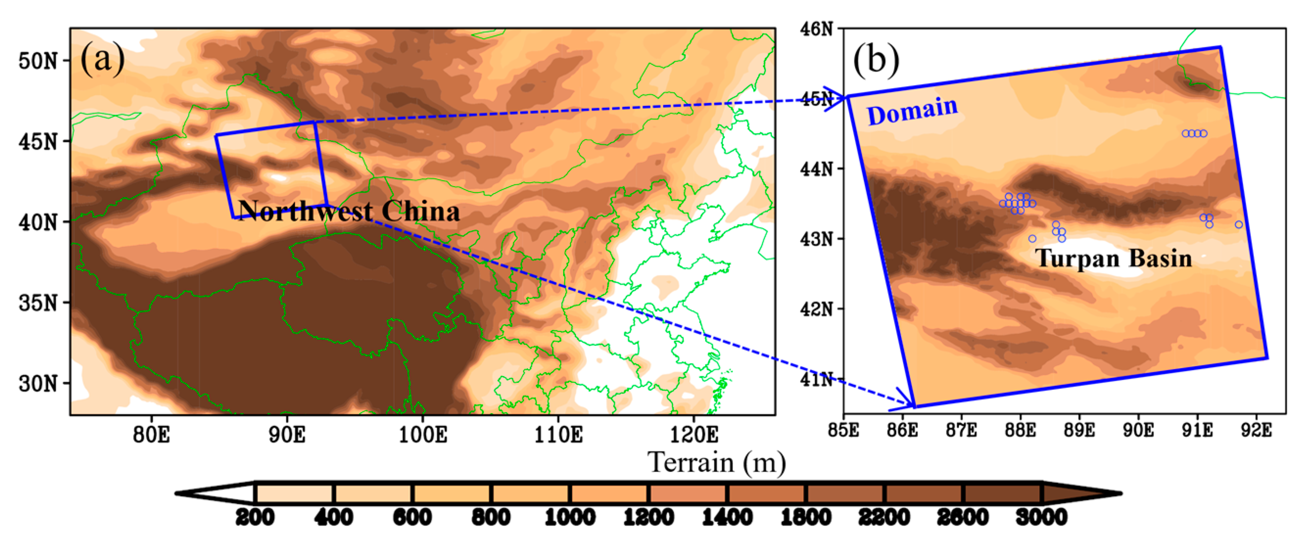
2. Data, Model Configuration and Methods

The hourly, 0.125° × 0.125° atmospheric model high resolution 10-day forecast from the European Centre for Medium-Range Weather Forecasts (ECMWF) [39] was used in this study for generating the initial and boundary conditions to drive the WRF model (

Table 1. Model configurations of the control run and two test runs. RRTMG = Rapid Radiative Transfer Model for General circulation models. NOAH = National Centers for Environmental Prediction, Oregon State University, Air Force, and Hydrology Lab.

	Control Run	Test 01	Test 02
Planetary boundary layer scheme	YSU [33]	YSU	YSU
Microphysics scheme	Ferrier [35]	Ferrier	Ferrier
Land surface model	NOAH [36]	NOAH	NOAH
Short wave radiation scheme	RRTMG [37]	RRTMG	RRTMG
Long wave radiation scheme	RRTMG [38]	RRTMG	RRTMG
TopoWind model	none	topo_wind = 1	topo_wind = 2

). The hourly 0.25° × 0.25° ECMWF ERA5 (ECMWF Reanalysis the 5th version; https://www.ecmwf.int/en/forecasts/datasets/reanalysis-datasets/era5 (accessed on 1 June 2021)) reanalysis data (Hersbach and Dee, 2016) and the wind-farm wind speed observation were used to evaluate the simulation results by different model configurations. In this study, the 7 variables shown in

Table 2. Performances of Test 01 and Test 02 relative to that of control run (%). u10 = 10-m zonal wind; v10 = 10-m meridional wind; spd10 = 10-m wind speed; t2 = 2-m temperature; slp = sea level pressure; z50 = 500-hPa geopotential height; t50 = 500-hPa temperature.

		u10		v10		spd10		t2		slp		z50		t50
		24 h	48 h	24 h	48 h	24 h	48 h	24 h	48 h	24 h	48 h	24 h	48 h	24 h	48 h
Test 01	CORC	+3	+3	+3	+3	+6	+4	+1	+0	+1	+1	+1	+1	+1	+1
	RMSE	−4	−5	−4	−6	−4	−6	−4	−4	−4	−2	−3	−2	−2	−2
Test 02	CORC	+8	+8	+7	+8	+9	+9	+3	+1	+2	+4	+2	+2	+3	+2
	RMSE	−11	−13	−13	−14	−13	−14	−8	−7	−9	−8	−8	−7	−5	−4

, i.e., 10-m zonal wind (u10), 10-m meridional wind (v10), 10-m wind speed (spd10), 2-m temperature (t2), sea level pressure (slp), 500-hPa geopotential height (z50), 500-hPa temperature (t50) were evaluated by using the ERA5 reanalysis data; and the 70-m wind speed was evaluated by using wind-farm observations. Of these, t2 and slp were evaluated as they acted as dominant factors for the variations of near-surface wind field [40,41,42,43,44]; z50 and t50 were evaluated as they served as important background environment for near-surface wind field [1].

The multi-scale processes related to the lower-level wind speed in Northwest China were simulated by using the WRF version 4.1.1. A total of 3 model configurations were used in this study as shown in Table 1. Of these, the control run used the model configuration that was selected from a series of comparisons (in our operational forecasting, we compared a total of 10 model configurations to determine the best configuration) as it showed overall the best performance in forecasting the near-surface winds. The Test 01 run was the same to the control run but used the TopoWind model with topo_wind = 1; the Test 02 run was the same to the control run but used the TopoWind model with topo_wind = 2. These two runs were used to evaluate the performances of the two TopoWind models (discussed in the introduction) in improving the near-surface wind forecasts. Only one domain with 169 × 169 grid points (Figure 1), 51 vertical levels, and a horizontal resolution of 3 km × 3 km were used in the simulations. The simulation period was from 12:00 UTC 01 to 12:00 UTC 28 October 2020, with the WRF model started at 12:00 UTC each day (there was 28 runs for a set of model configuration) and ran for 48 h.

From WRFv3.4 on, the WRF provided a TopoWind model that was associated with the YSU PBL scheme [33] to improve the topographic effects on the near-surface winds. There was a total of three options for the YSU PBL scheme: (i) topo_wind = 0, which did not include the additional topographic effects from the TopoWind model in the near-surface wind calculation; (ii) topo_wind = 1, which included the standard deviation of the subgrid-scale orography in the near-surface wind calculation; and (iii) topo_wind = 2, which used a method the same as that of topo_wind = 1 to calculate the near-surface winds, but meanwhile enhanced the calculation of the friction velocity by including the subgrid terrain variance. More detailed information about the TopoWind models can be found in literatures [10,31,32].

In this study, the root mean square error (RMSE) and the correlation coefficient (CORC) were used to evaluate the performances of different model configurations:

$$\mathrm{RMSE}=\sqrt{\frac{1}{N}{{\displaystyle \sum }}_{i=1}^N{\left(F_i-O_i\right)}^2}$$

(1)

$$\mathrm{CORC}={{\displaystyle \sum }}_{i=1}^N\left(F_i-\overline{F}\right)\left(O_i-\overline{O}\right)/\sqrt{{{\displaystyle \sum }}_{i=1}^N{\left(F_i-\overline{F}\right)}^2{{\displaystyle \sum }}_{i=1}^N{\left(O_i-\overline{O}\right)}^2}$$

(2)

where N is the total number used for calculation (e.g., for evaluation of the 24-h forecast, N = 24, as we used hourly output and hourly ERA5/observation for evaluation); F_i is the forecast at time i; O_i is the reanalysis/observation at time i. The RMSE was utilized to evaluate the forecast’s performance in reproducing the magnitude of a meteorological variable, and the CORC was used to evaluate the forecast’s performance in representing its variational trend. For calculating RMSE and CORC, because the resolution of WRF simulation was much higher than that of ERA5 reanalysis data, firstly, we interpolated the WRF output into 0.25° × 0.25° resolution (by using bilinear interpolation), which was the same as that of ERA5 reanalysis data. Then, for the points within the simulation domain (the blue box shown in Figure 1b), (i) we calculated RMSEs and CORCs at each point; and (ii) we calculated the area average of the RMSEs and CORCs at all points within the simulation domain to get the area-averaged RMSE and CORC for comparing the performances of different model configurations. For the comparison using wind-farm observation, a similar approach was taken, during which we interpolated the WRF output into 24 wind-farm observational stations (Figure 1b) by using the bilinear interpolation.

3. Comparisons among Different Model Configurations

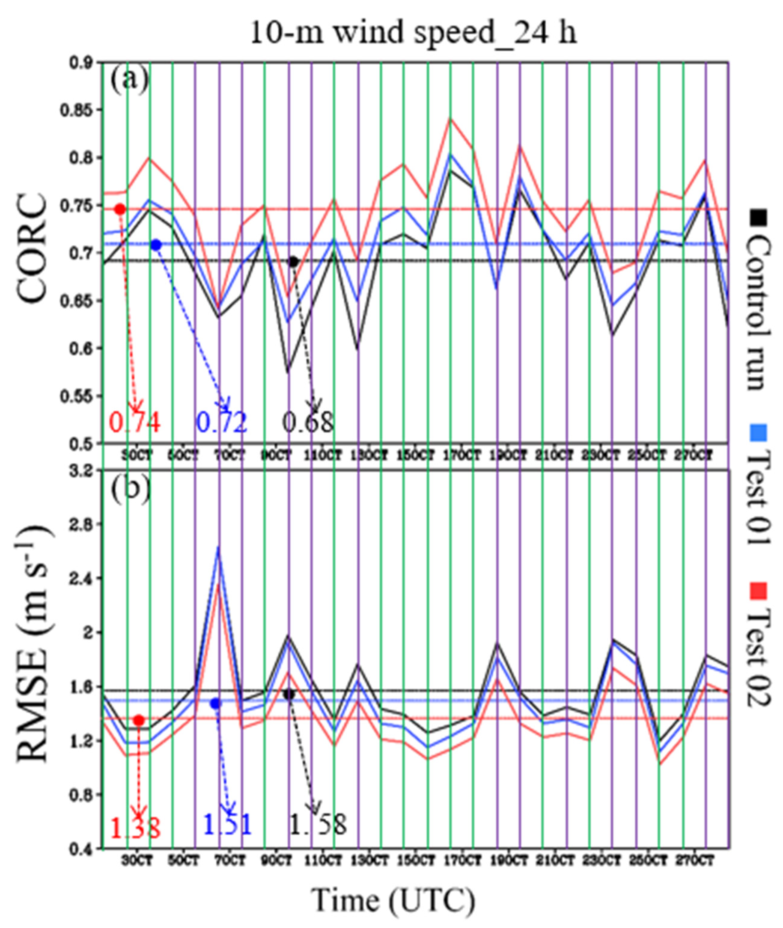
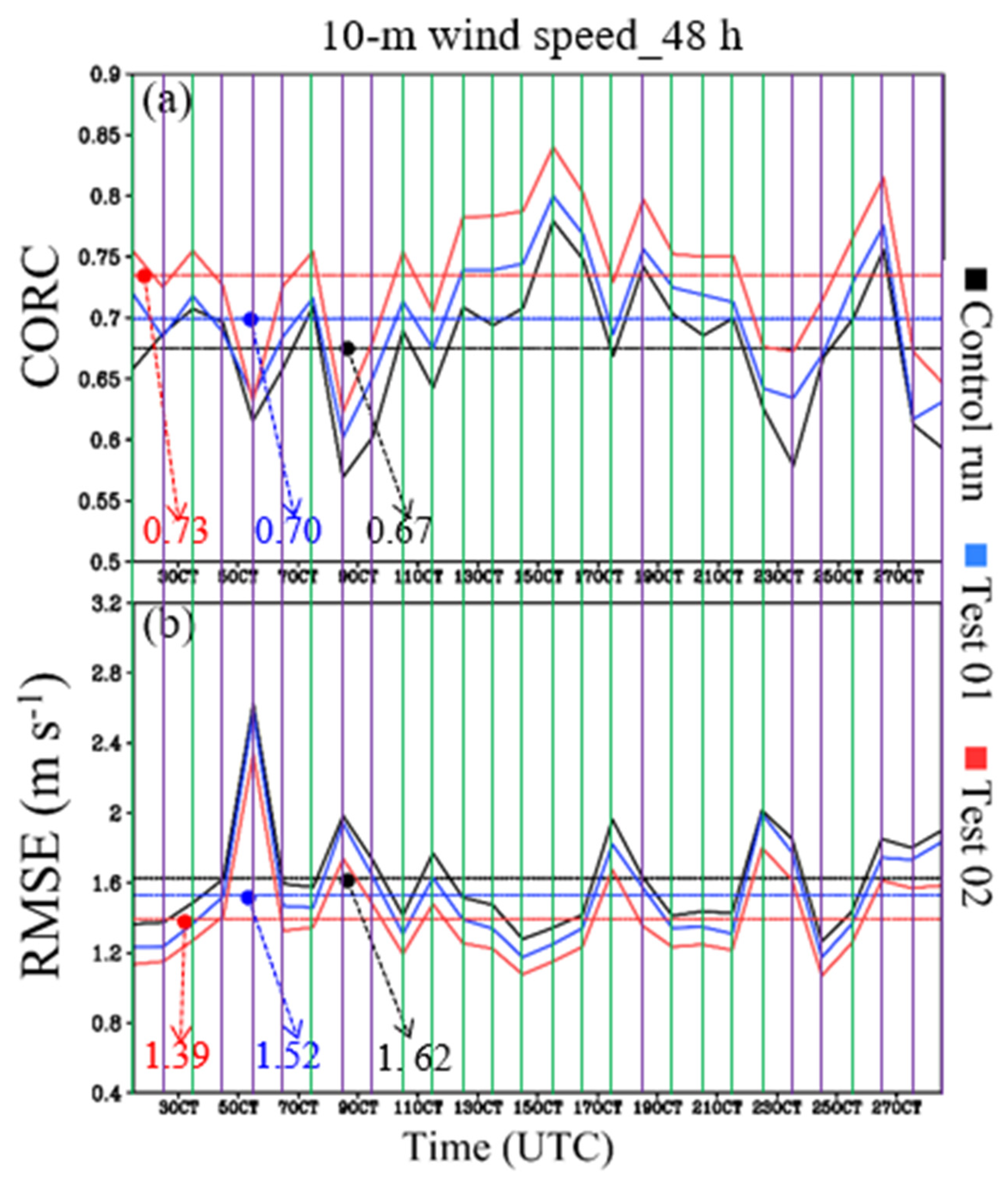
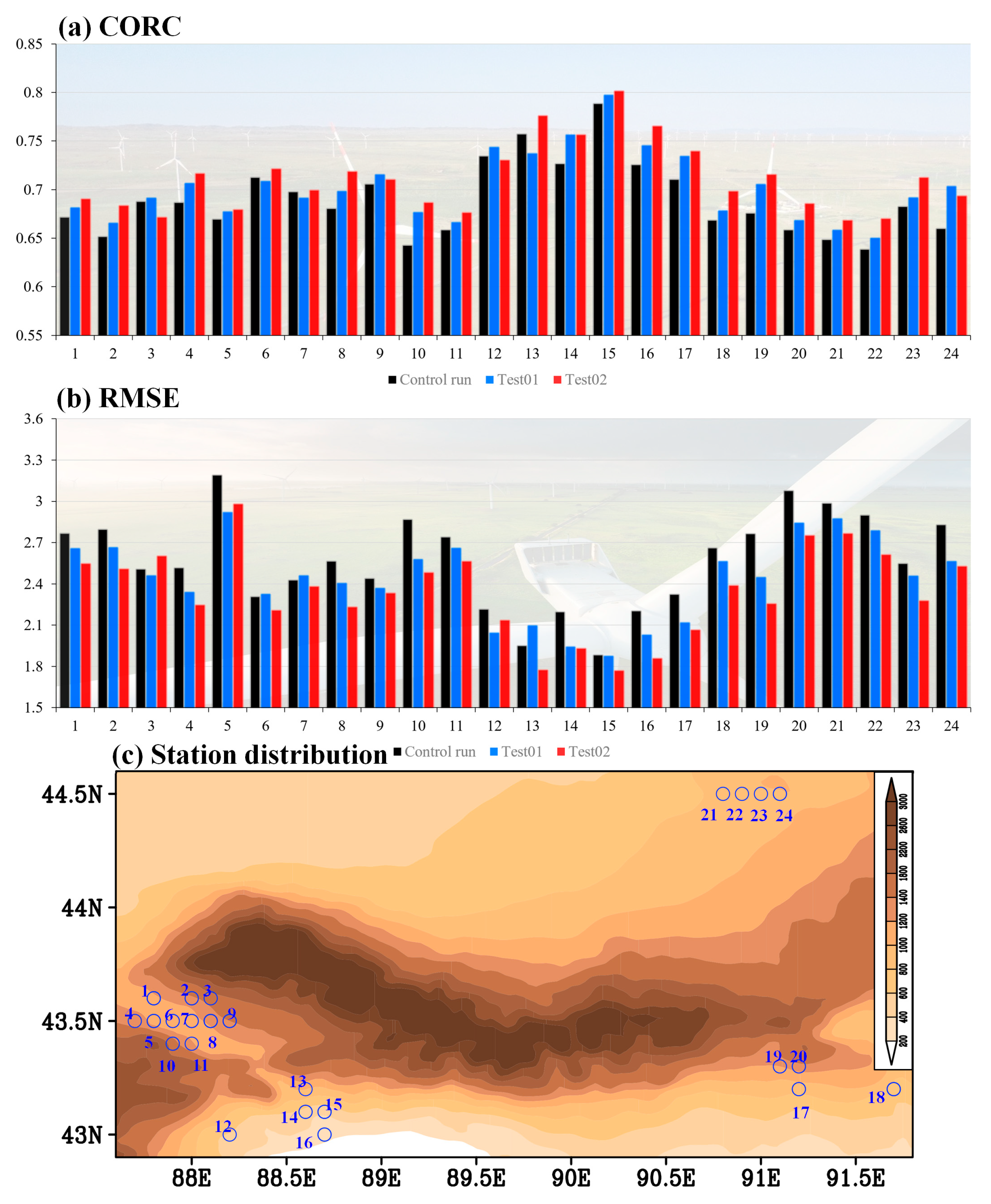
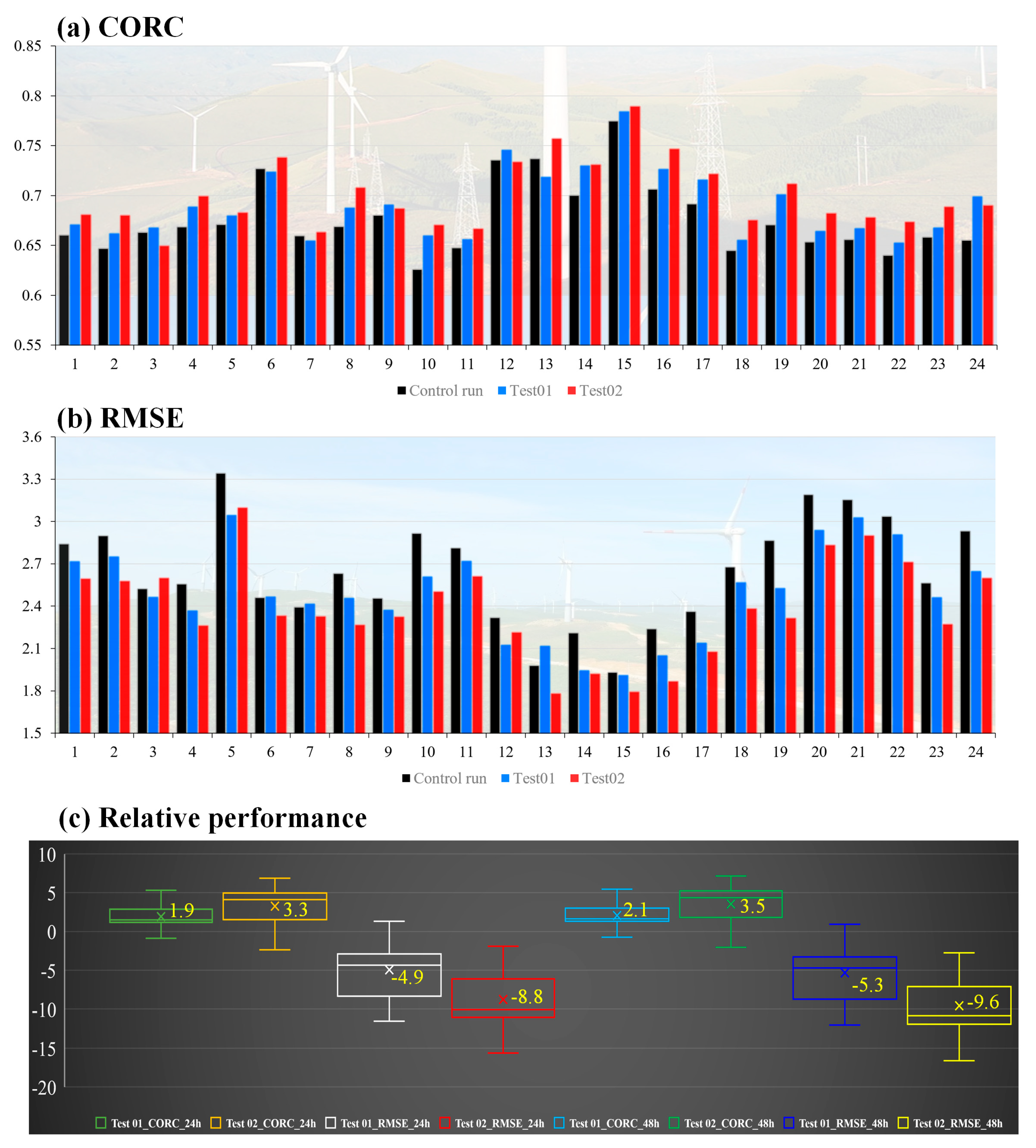
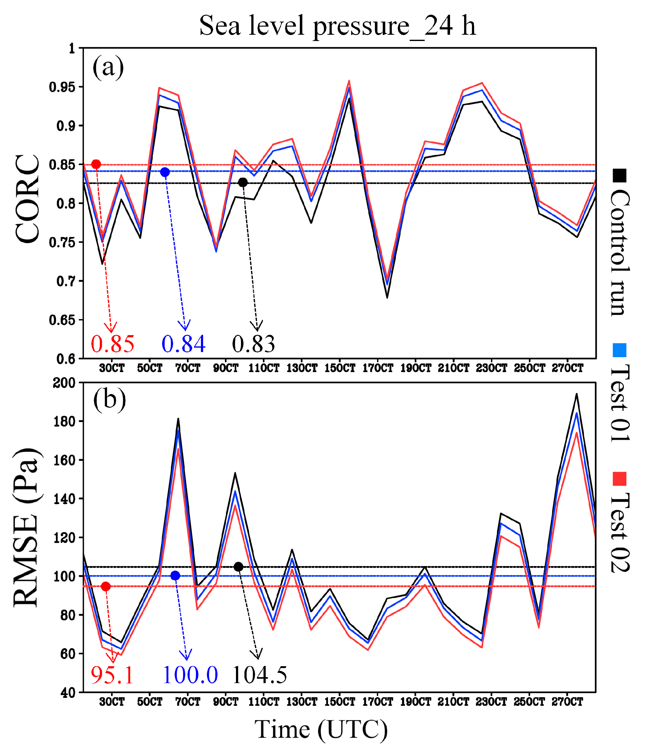
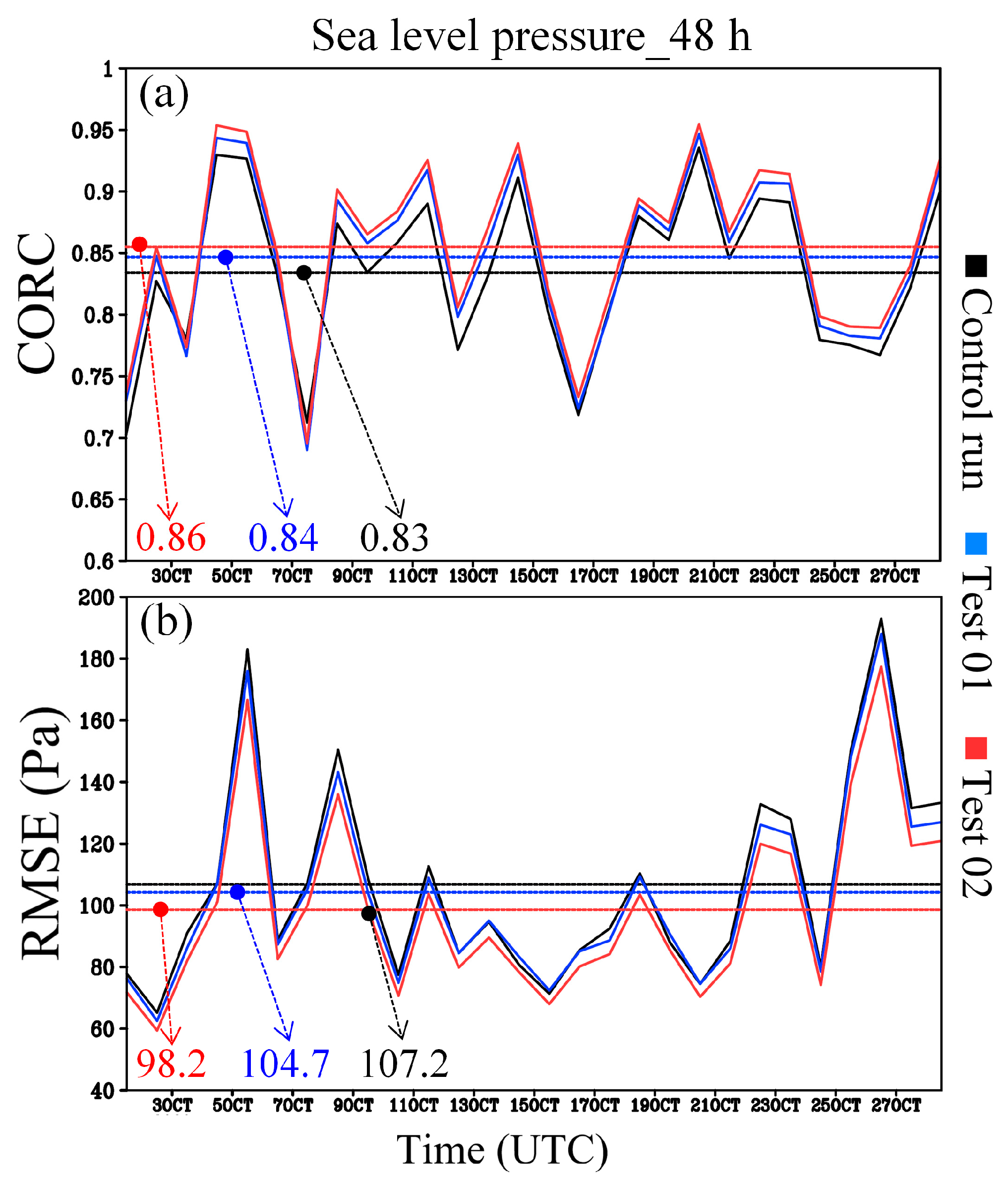
3.1. Evaluation of the 10-m Wind Speed

As the primary purpose of this study is to evaluate the performance of the TopoWind model in forecasting the near-surface wind (we used 10-m and 70-m wind speed as representatives) under the complex terrain conditions over Northwest China, we first evaluated the near-surface wind forecast. From Figure 2 it can be seen that, for the spd10 forecast within 0–24 h (24-h forecast for convenience), the CORC and RMSE varied with time notably. Overall, for the 28 control runs (Section 2), their largest CORC (~0.78) appeared in the forecast started from 12:00 UTC 16 October (Figure 2a), the smallest CORC (~0.57) appeared in the forecast started from 12:00 UTC 09 October, and the mean CORC among 28 control runs was ~0.68. The variation of control-runs’ RMSE showed an obvious inverse correlation (the correlation coefficient was around −0.69) to their CORC (Figure 2b), implying that those forecasts with larger CORCs tended to have smaller RMSEs, and vice versa. Detailed comparisons showed that the smallest RMSE (~1.2 m s⁻¹) appeared in the forecast started from 12:00 UTC 25 October (Figure 2b), the largest RMSE (~2.6 m s⁻¹) appeared in the forecast started from 12:00 UTC 06 October, and the mean RMSE was ~1.6 m s⁻¹. Thus, it can be concluded that the best/worst forecast in terms of CORC and the best/worst forecast in terms of RMSE were usually different. In order to differ good forecasts from bad forecasts, we used the following definition: (i) for a series of forecasts, if one of them satisfied: (i) its CORC was larger than the mean CORC of these forecasts, and (ii) its RMSE was smaller than the mean RMSE of these forecasts at the same time, then, it is a good forecast; otherwise, it was a bad forecast. As Figure 2 shows, ~50% of the control runs were good forecasts. A similar situation was found in the spd10 forecast within 24–48 h (48-h forecast for convenience; Figure 3): (i) those forecasts with larger/smaller CORCs tended to have smaller/larger RMSEs (the correlation coefficient was around −0.63); (ii) the best/worst forecast in terms of CORC and the best/worst forecast in terms of RMSE were usually different; and ~50% of the control runs were good forecasts.

For 24-h/48-h forecast, compared to each of the 28 control runs, almost all Test-01 and Test-02 runs showed an increase in their CROCs and a decrease in their RMSEs (Figure 2), with the changes of the Test-02 run larger than those of the Test-01 run. This means that, overall, both the TopoWind models could improve the 10-m wind speed forecasts within 0–24 h and 24–48 h, and the topo_wind = 2 option showed a better performance than that of the topo_wind = 1 option. In order to compare the improvements of Test-01 and Test-02 runs relative to the control runs, we defined the relative performance (RP) as follows:

$${\mathrm{RP}}_{\mathrm{CORC}}=\frac{{\overline{\mathrm{CORC}}}_{\mathrm{test}}-{\overline{\mathrm{CORC}}}_{\mathrm{control}}}{{\overline{\mathrm{CORC}}}_{\mathrm{control}}}$$

(3)

$${\mathrm{RP}}_{\mathrm{RMSE}}=\frac{{\overline{\mathrm{RMSE}}}_{\mathrm{test}}-{\overline{\mathrm{RMSE}}}_{\mathrm{control}}}{{\overline{\mathrm{RMSE}}}_{\mathrm{control}}}$$

(4)

where subscripts CORC and RMSE stand for the factors that are calculated, the overbar denotes the mean values among all control, Test 01, and Test-02 runs, respectively, the subscript “test” stands for Test 01 or Test 02, and the subscript “control” represents the control run. From its definition, the RP can represent changes in forecast accuracy.

As shown in Table 2, compared to the control run, on average, for the forecast within 0–24 h, Test 01 increased the mean CORC by ~6% and reduced the mean RMSE by ~4%; and Test 02 increased the mean CORC by ~9% and reduced the mean RMSE by ~13%. For the forecast within 24–48 h, Test 01 increased the mean CORC by ~4% and reduced the mean RMSE by ~6%; and Test 02 increased the mean CORC by ~9% and reduced the mean RMSE by ~14%. Therefore, it can be concluded that, (i) both topo_wind = 1 and topo_wind = 2 options could improve the 10-m wind speed forecast (particularly for reducing the RMSE) under the complex terrain conditions over Northwest China (Table 2); (ii) the improvements were similar for the 24-h (4–13%) and 48-h forecasts (4–14%); and (iii) the topo_wind = 2 option (9–14%) showed a more notable improvement than the topo_wind = 1 (4–6%).

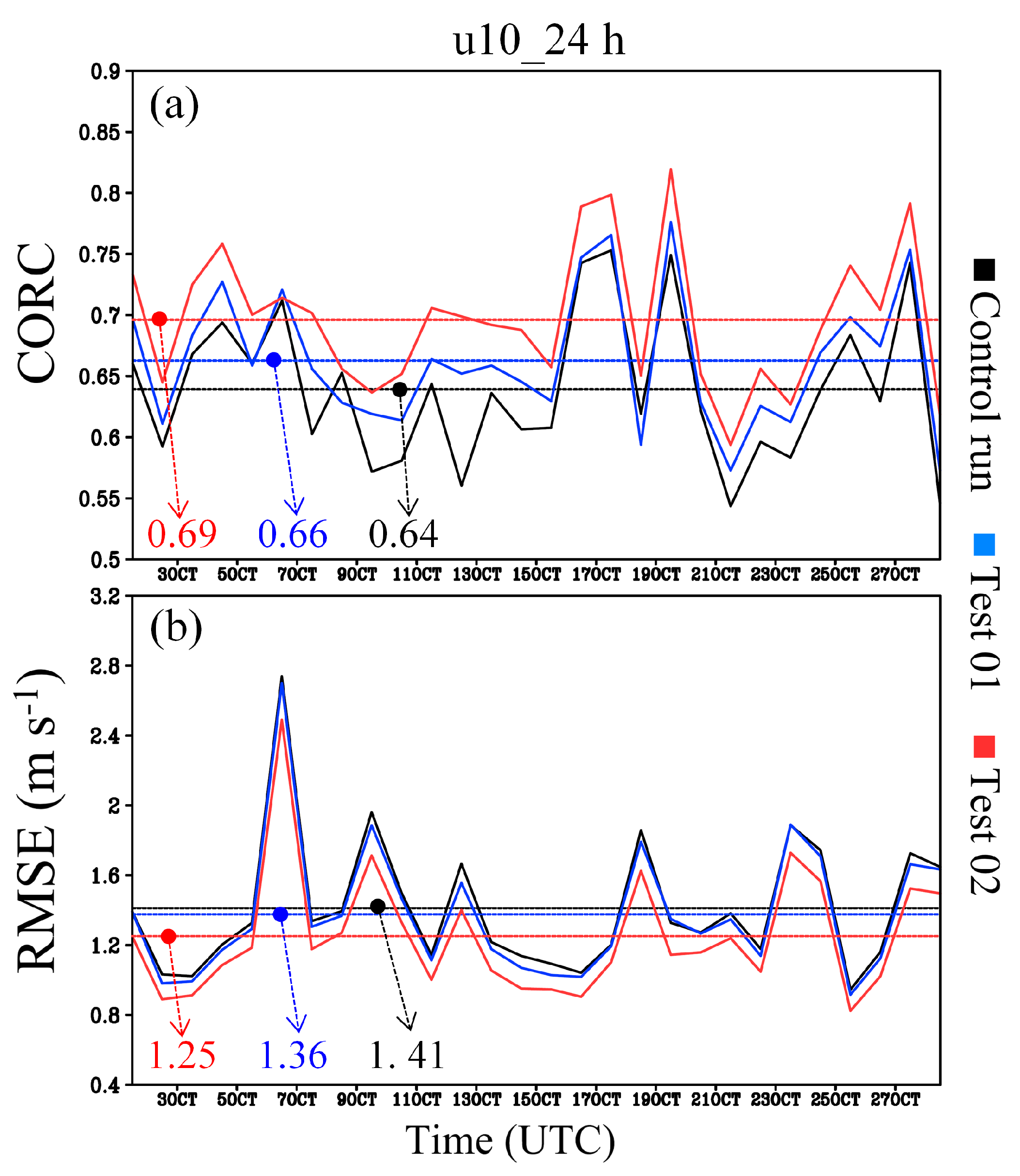
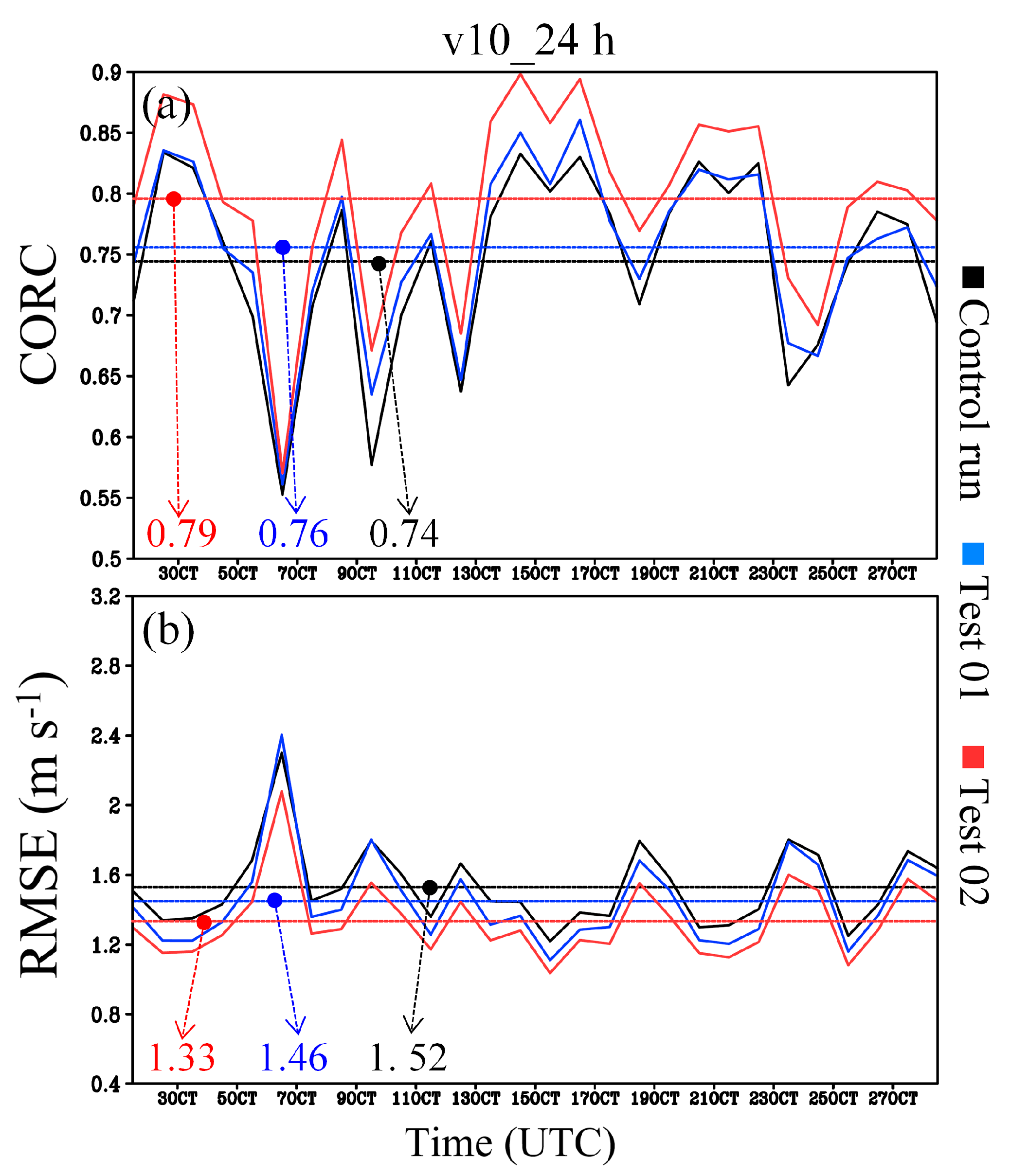
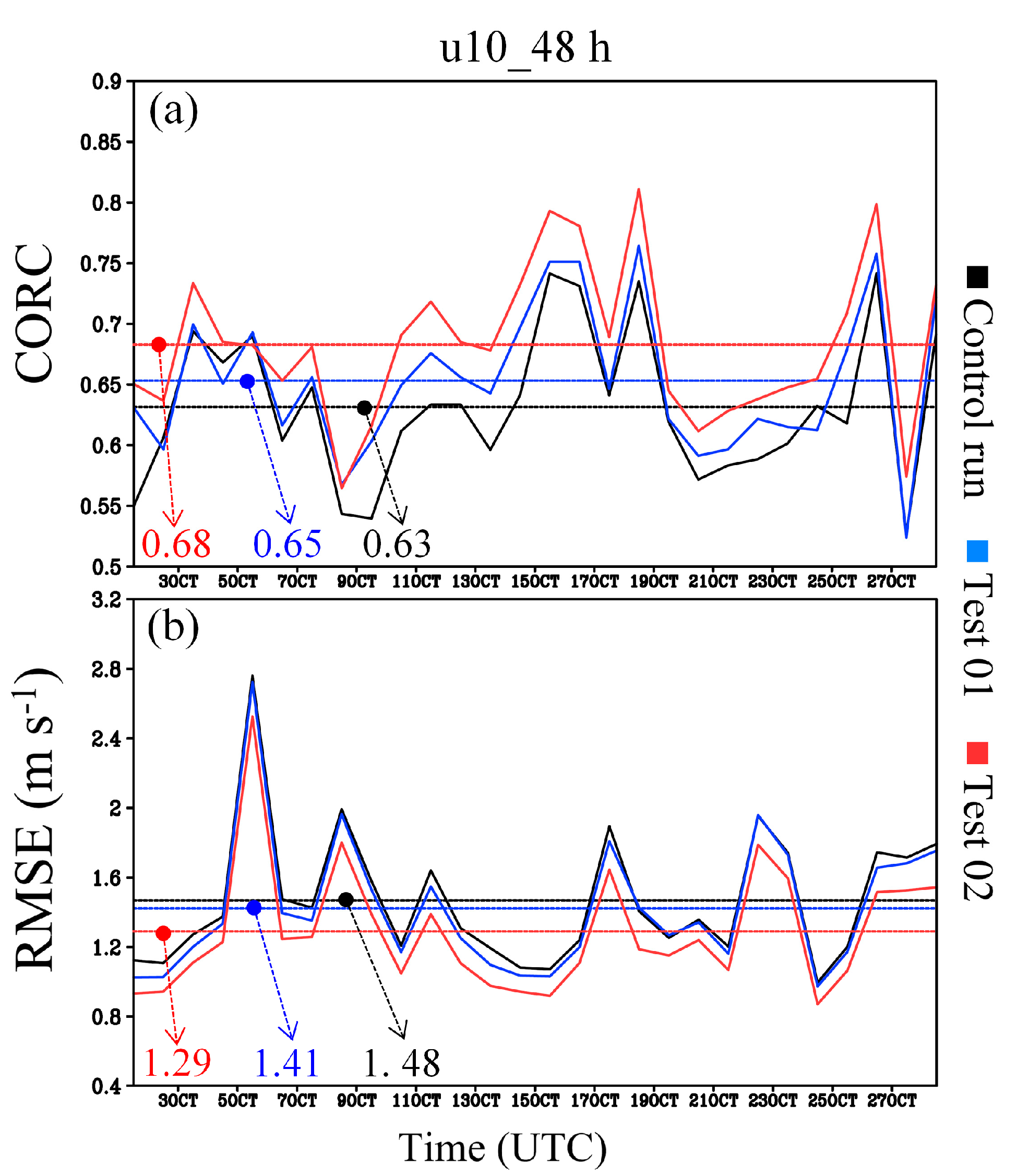
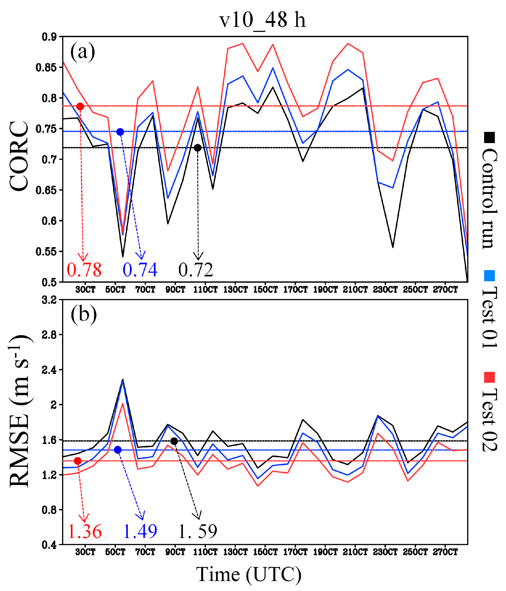
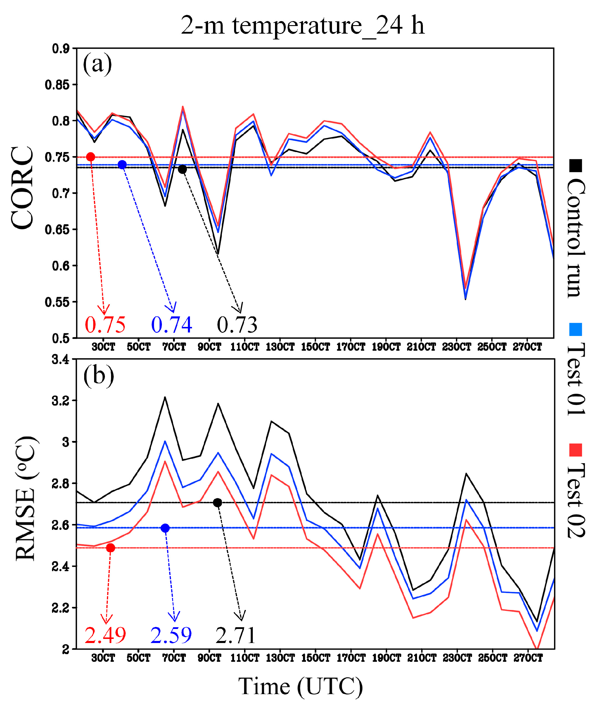
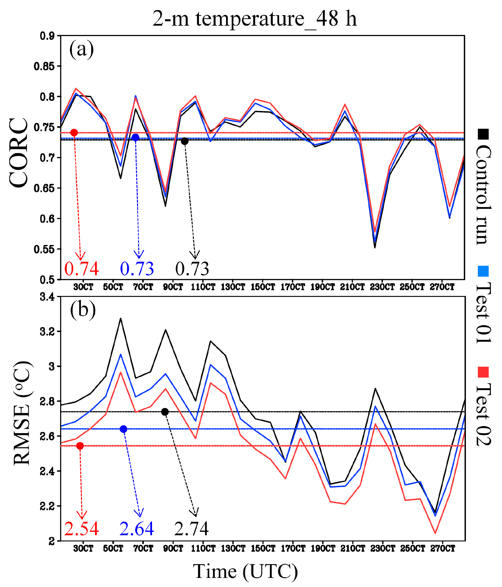
3.2. Evaluation of the 10-m Zonal and Meridional Wind

Wind is a vector which could be decomposed into the zonal wind and the meridional wind. As illustrated in

Table 3. Correlation coefficients between the CORCs/RMSEs of various variables (i.e., u10 and v10) and the CORC/RMSE of the 10-m wind speed. u10 = 10-m zonal wind; v10 = 10-m meridional wind.

		Control Run		Test 01		Test 02
		24 h	48 h	24 h	48 h	24 h	48 h
u10	CORC	0.62	0.63	0.63	0.64	0.65	0.67
	RMSE	0.91	0.93	0.92	0.94	0.95	0.96
v10	CORC	0.81	0.83	0.83	0.85	0.84	0.87
	RMSE	0.86	0.88	0.89	0.90	0.91	0.93

, in terms of CORC, for all runs, the v10 forecast showed a much larger correlation coefficient with the 10-m wind speed than that of the u10 forecast, whereas, in terms of RMSE, the u10 forecast had a larger correlation coefficient. This means that the forecast of v10 was more important to the variational trend of the 10-m wind speed and the forecast of u10 was more important to the magnitude of the 10-m wind speed. Overall, Test 02 had the largest correlation coefficients of CORCs and RMSEs of u10 and v10 for both 24-h and 48-h forecasts (Table 3), whereas, those of the control run were the smallest.

Comparing Figure 4 and Figure 5 to Figure 2 shows that, on average, the CORC of the 10-m wind speed (Figure 2) was between the CORC of u10 (Figure 4) and CORC of v10 (Figure 5), with the former smaller than the latter. This was true for the Control run, Test 01 and Test 02, as both the zonal and meridional winds were important to the variational trend of 10-m wind speed. In contrast, for the RMSE, that of the 10-m wind speed (Figure 2) was smaller than those of u10 and v10 (Figure 4 and Figure 5). This was because that the 10-m wind speed was larger than u10 or v10. From Table 2 it can be found that, for the 24-h forecasts, Test 01 increased the CROCs of u10 and v10 forecasts by ~3%, and reduced the RMSEs of u10 and v10 forecasts by ~4%. Test 02 showed a much better performance, as it increased the CROCs of u10 and v10 forecasts by ~8%, and reduced the RMSEs of u10 and v10 forecasts by ~11–13%. Similar situations were found for the 48-h forecasts (cf., Figure 4, Figure 5, Figure 6 and Figure 7), except that the RMSEs of u10 and v10 showed more notable improvements than those of 24-h forecasts (Table 2). Therefore, it can be concluded that, on average, both TopoWind models could improve the forecasts of u10 and v10 (particularly for the RMSE), with the topo_wind = 2 option showed a better performance than that of the topo_wind = 1 option.

3.3. Evaluation of the 70-m Wind Speed

This study used a total of 24 wind-farm observational stations (Figure 8c) to evaluate the forecast of 70-m (the height of wind-farm’s wind observation) wind speed. The simulated 70-m wind speed was produced by vertical interpolation using the wind speeds at the two sigma levels that were the closest to the height of 70-m. As Figure 8a,b and Figure 9a,b show, for a same set of model configuration (e.g., the Control run, Test 01 or Test 02 shown in Table 1), its performance at different stations were different. Different geographical positions (Figure 8) of these stations were key reasons for their different forecast accuracy. Comparisons among all 24 stations show that, stations #12-#16 generally showed larger CORCS and smaller RMSEs than those of other stations (Figure 8a,b and Figure 9a,b). These stations were mainly located south of the mountain, where terrain was below 1000 m. In addition, different weather systems (i.e., systems that produced the wind) were also an important reason for the different forecast accuracy at different stations.

In terms of CORC, for the 24-h forecast, the CORCs of the control run varied from 0.63 (the wind-farm station #22) to 0.79 (#15), with a mean value of ~0.69 (Figure 8a). The CORCs of the Test 01 varied from 0.65 (the wind-farm station #22) to 0.80 (#15), with a mean value of ~0.70. The CORCs of the Test 02 varied from 0.67 (the wind-farm station #21) to 0.80 (#15), with a mean value of ~0.71. As Figure 9c shows, on average, Test 01 and Test 02 increased the 24-station mean CORC by 1.9% and 3.3%, respectively. For the 48-h forecast, similar situations were found (cf., Figure 8a and Figure 9a), except that the CORCs were mainly smaller than those of the 24-h forecast. Overall, Test 01 and Test 02 increased the 24-station mean CORC by 2.1% and 3.5%, respectively (Figure 9c), which were larger than those of the 24-h forecast. All in all, as mentioned above, the TopoWind models could improve the forecast of the variational trends of the 70-m wind speed, with the topo_wind = 2 option showing a better performance.

In terms of RMSE, for the 24-h forecast, the RMSEs of the control run varied from 1.9 (the wind-farm station #15) to 3.2 (#5), with a mean value of ~2.6 (Figure 8b). The RMSEs of the Test 01 varied from 1.9 (the wind-farm station #15) to 2.9 (#5), with a mean value of ~2.4. The RMSEs of the Test 02 varied from 1.8 (the wind-farm station #15) to 3.0 (#5), with a mean value of ~2.3. As Figure 9c shows, on average, Test 01 and Test 02 reduced the 24-station mean RMSE by 4.9% and 8.8%, respectively. For the 48-h forecast, similar situations were found (cf., Figure 8b and Figure 9b), except that the RMSEs were mainly larger than those of the 24-h forecast (i.e., forecast accuracy was lower). Overall, Test 01 and Test 02 reduced the 24-station mean RMSE by 5.3% and 9.6%, respectively (Figure 9c), which was larger than those of the 24-h forecast (i.e., improvement for the 48-h forecast was more notable). All in all, as mentioned above, the TopoWind models could improve the forecast of the magnitude of the 70-m wind speed, with the topo_wind = 2 option showing a better performance.

4. Discussion on the Forecast Accuracy of Near-Surface Winds

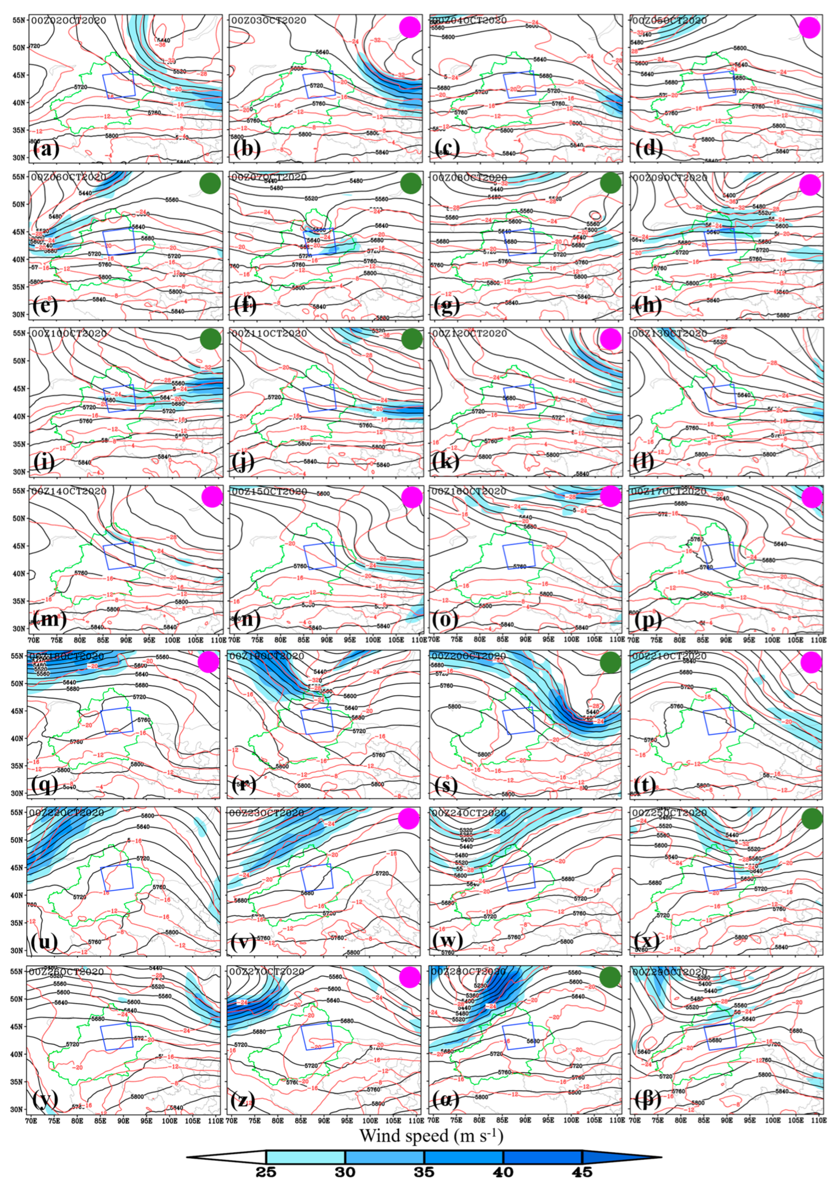
4.1. Effects of Different Weather Systems

It is known that, for the same model configuration, its performances in forecasting the wind field associated with different weather systems were notably different [8,15,34,35,36,37]. As this study focused on October 2020, it is necessary to first know the main pattern of the surface wind filed during this period. As Figure 10a shows, in terms of the temporal mean state, the simulation domain was governed by different wind field. Overall, the northerly winds were dominant, and westerly and easterly winds also appeared, particularly in the regions around 44° N 91° E and 42° N 91° E. The winds with larger/smaller speed mainly appeared in the eastern/western section of the simulation domain. In terms of the spatial mean state, it can be found that the fluctuations of the wind were notable (black line in Figure 10b), which indicated the surface winds changed significantly. For the zonal wind (red line in Figure 10b), the period occupied by the negative values was similar to that by the positive values. This means that the simulation domain was controlled alternately by easterly and westerly winds. For the meridional wind (blue line in Figure 10b), negative values appeared much more frequently than the positive values, which means that the northerly winds were dominant.

As different weather systems were associated with different wind fields [1,34,35,36,37], we summarized the good and bad forecasts according to their background environments. As Figure 2 and Figure 3 show, for the 24-h/48-h forecast started at each day (there were 28 runs in the Test-01/Test-02), if CORCs of Test 01 and Test 02 were above their corresponding mean CORCs (among their corresponding 28 runs), and RMSEs of Test 01 and Test 02 were below their corresponding mean RMSEs, it was regarded as a good forecast; whereas, if CORCs of Test 01 and Test 02 were below their corresponding mean CORCs, and RMSEs of Test 01 and Test 02 were above their corresponding mean RMSEs, it was regarded as a bad forecast. If the forecast was good both for the 24-h and 48-h runs, it was marked with a purple closed circle as shown in Figure 11. If the forecast was bad both for the 24-h and 48-h runs, it was marked with a green closed circle. Comparison of the situations with purple and green circles (Figure 11) shows that, during good forecasts, the simulation domain was mainly controlled by high-pressure systems such as a ridge (Figure 11b) or a closed high-pressure center (Figure 11p), and the upper-level jet was mainly far from the domain (Figure 11k). In contrast, during bad forecasts, the simulation domain was mainly controlled by low-pressure systems such as a trough (Figure 11f), and the upper-level jet was mainly close to the domain (Figure 11s). High-pressure systems were generally more stable than lower-pressure systems [1]; and upper-level jet could affect lower-level systems by its secondary circulation (regions close to the upper-level jet were affected notably). These were key reasons for the differences between good and bad forecasts.

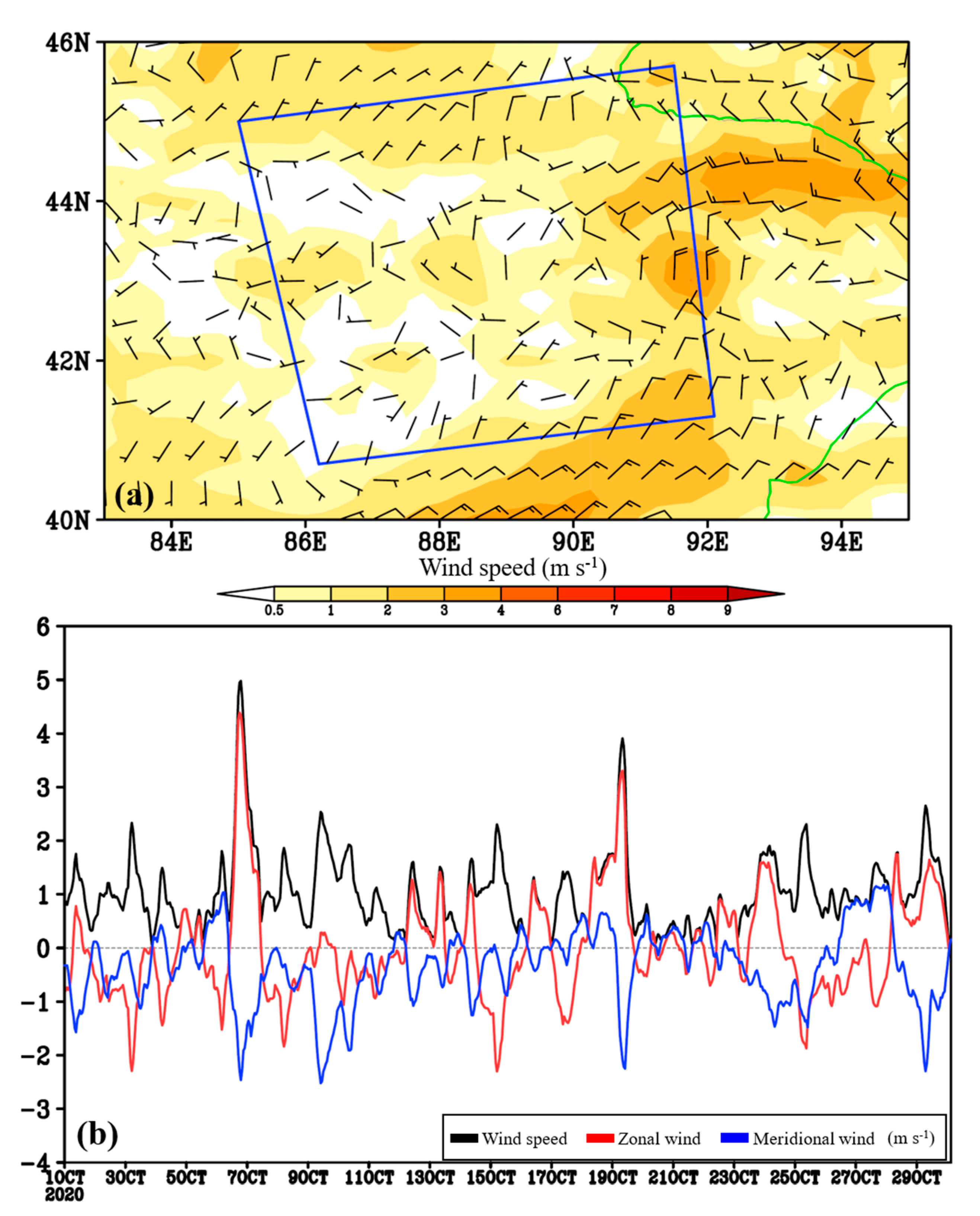
4.2. Effects of Near-Surface Features

As discussed in Section 3, both TopoWind models could improve the near-surface wind forecast. Possible reasons were discussed in this section. As Figure 12a and Figure 13a illustrate, for both 24-h and 48-h forecast, on average, Test 01 and Test 01 showed improvements in forecasting the variational trends of slp (i.e., CORCs increased). In addition, as Figure 12b and Figure 13b depict, improvements of the forecast of the magnitude of slp were more notable (i.e., RMSEs reduced), particularly for the topo_wind = 2 option. This means that the TopoWind models could improve the slp forecast. This is an important reason for the improvement of the wind speed forecast, as slp was crucial in determining wind speed (through doing work by the pressure gradient force; Holton 2004).

From Figure 14 and Figure 15, although the TopoWind models showed unobvious effects in improving the forecast of the variational trends of the 2-m temperature, they showed notable contributions in improving the forecast of the 2-m temperature’s magnitude, particularly for the topo_wind = 2 option. A better forecast of 2-m temperature field contributed to reach a better forecast of near-surface wind speed, as baroclinity (which could be represented by temperature gradient) could enhance/weaken the near-surface wind speed through the baroclinic energy conversion [1,34]. All in all, as discussed above, it can be concluded that the TopoWind models could improve the forecast of slp and 2-m temperature field, which finally resulted in the improvements of near-surface wind speed forecast. Moreover, the topo_wind = 2 option was overall better than the topo_wind = 1 option in the forecast of near-surface wind. This was mainly because that the former had included the subgrid terrain variance in calculating the friction velocity in addition to the procedures added by the latter.

4.3. Limitations of This Study

As discussed above, this study has shown the ability of two TopoWind models in improving the forecast accuracy of the near-surface winds under the complex terrain conditions over Northwest China. To better understand this conclusion, one needs to know the limitations of this study. (i) The result was only based on a forecast period of around a month. As different weather systems were crucial to the forecast accuracy, we suggest to conduct more tests in the future. These tests should contain more types of weather systems, and also should consider the influences of seasonal variations (this study only focused on autumn). (ii) The simulation domain of this study was small relative to the Northwest China, therefore more regions in the Northwest China should be used in the evaluations of the TopoWind models. Properly addressing (i) and (ii) will contribute to the final improvement of the near-surface wind forecast over Northwest China. (iii) We only focused on the near-surface features to understand why the TopoWind models could improve the near-surface winds’ forecast. In fact, as the weather systems that caused the strong winds usually had a thick vertical extent, more vertical levels (such as 700 hPa, 500 hPa) should also be used in the analyses. This will enhance the understanding of the TopoWind models, which is useful for improving them in the future.

5. Conclusions

The Northwest China is a region with the most abundant WE in East Asia and even the world. Because of the WE’s notable features of randomness, diversity and uncontrollability, the effective utilization of the WE needs accurate near-surface wind forecasts. Although the WRF model had been widely used for wind forecasts worldwide, its forecasts of near-surface wind still showed notable errors. In order to improve the simulation accuracy of the low-level wind speed, two TopoWind models were developed and added to the YSU PBL scheme. This study conducted the first test to check whether the two TopoWind models could improve the near-surface wind prediction under complex terrain conditions over Northwest China. This contributes to making full use of WE in Northwest China and to improving the efficiency of wind power generation systems.

Based on three groups (each group had 28 runs) of forecasts (i.e., Control run, Test 01 and Test 02) started at 12:00 UTC of each day (ran for 48 h) during the period of 01–28 October 2020, we found that: (i) the forecast accuracy of 10-m wind speed varied each day, with ~50% of them belonged to good forecasts; those forecasts with larger CORCs tended to have smaller RMSEs (i.e., they were in an inverse correlation), and vice versa; both TopoWind models could improve the 10-m wind speed forecasts under the complex terrain conditions over Northwest China, particularly for reducing the RMSE, and the topo_wind = 2 option showed a better performance (improve the forecast accuracy by 9–14%) than that of the topo_wind = 1 option (4–6%). (ii) The forecast of 10-m meridional wind was more important to the forecast of the variational trend of the 10-m wind speed, and the forecast of 10-m zonal wind was more important to the forecast of the magnitude of the 10-m wind speed; on average, both TopoWind models could improve the forecasts of 10-m meridional and zonal winds (particularly for reducing RMSE), with the topo_wind = 2 option showed a better performance (improve the forecast accuracy by 7–14%) than that of the topo_wind = 1 option (3–6%). (iii) Geographical features (stations located south of the mountain, where terrain was below 1000 m, tended to have more accurate forecast) were crucial to the forecast accuracy of the 70-m wind speed; the two TopoWind models could improve the forecasts of the 70-m wind speed, particularly for lowering the RMSE, with the topo_wind = 2 option shown a better performance (improve the forecast accuracy by 3–10%). (iv) Different weather systems were crucial to the forecast accuracy, good forecasts tended to appear when the simulation domain was mainly controlled by high-pressure systems with the upper-level jet far from it; bad forecasts tended to appear when the simulation domain was mainly controlled by low-pressure systems with the upper-level jet close to it. (v) The two TopoWind models could improve the forecast of sea level pressure (which affected the wind field through the work done by the pressure gradient force) and 2-m temperature field (which influenced the wind field through the baroclinic energy conversion), which finally resulted in the improvements of near-surface wind speed forecast.

References

1. Holton, J.R. An Introduction to Dynamic Meteorology; Academic Press: San Diego, CA, USA, 2004. [Google Scholar]
2. Fu, S.M.; Yu, F.; Wang, D.H.; Xia, R.D. A comparison of two kinds of eastward-moving mesoscale vortices during the mei-yu period of 2010. Sci. China Earth Sci. 2013, 56, 282–300. [Google Scholar] [CrossRef]
3. Calif, R.; Schmitt, F.G.; Huang, Y. Multifractal description of wind power fluctuations using arbitrary order Hilbert spectral analysis. Phys. A Stat. Mech. Its Appl. 2013, 392, 4106–4120. [Google Scholar] [CrossRef]
4. Ahmad, T.; Zhang, D. A data-driven deep sequence-to-sequence long-short memory method along with a gated recurrent neural network for wind power forecasting. Energy 2022, 239, 122109. [Google Scholar] [CrossRef]
5. Fu, S.; Li, W.; Sun, J.; Zhang, J.; Zhang, Y. Universal evolution mechanisms and energy conversion characteristics of long-lived mesoscale vortices over the Sichuan Basin. Atmos. Sci. Lett. 2015, 16, 127–134. [Google Scholar] [CrossRef]
6. Wu, C.; Luo, K.; Wang, Q.; Fan, J. Simulated potential wind power sensitivity to the planetary boundary layer parameterizations combined with various topography datasets in the weather research and forecasting model. Energy 2022, 239, 122047. [Google Scholar] [CrossRef]
7. Mughal, M.O.; Lynch, M.; Yu, F.; McGann, B.; Jeanneret, F.; Sutton, J. Wind modelling, validation and sensitivity study using Weather Research and Forecasting model in complex terrain. Environ. Model. Softw. 2017, 90, 107–125. [Google Scholar] [CrossRef]
8. Fu, S.M.; Sun, J.H.; Luo, Y.L.; Zhang, Y.C. Formation of long-lived summertime mesoscale vortices over central east China: Semi-idealized simulations based on a 14-year vortex statistic. J. Atmos. Sci. 2017, 74, 3955–3979. [Google Scholar] [CrossRef]
9. Wang, Q.; Luo, K.; Yuan, R.; Zhang, S.; Fan, J. Wake and performance interference between adjacent wind farms: Case study of Xinjiang in China by means of mesoscale simulations. Energy 2019, 166, 1168–1180. [Google Scholar] [CrossRef]
10. Yang, P.; Wang, X.; Wang, L.; Zhu, Y. A study on the applicability of WRF_TopoWind model to simulate the mountain wind speed of the low latitude plateau in China. J. Yunnan Univ. Nat. Sci. Ed. 2016, 38, 766–772. [Google Scholar]
11. Prosper, M.A.; Otero-Casal, C.; Fernández, F.C.; Miguez-Macho, G. Wind power forecasting for a real onshore wind farm on complex terrain using WRF high resolution simulations. Renew. Energy 2019, 135, 674–686. [Google Scholar] [CrossRef]
12. Cheng, X.L.; Li, J.; Hu, F.; Xu, J.; Zhu, R. Refined numerical simulation in wind resource assessment. Wind Struct. 2015, 20, 59–74. [Google Scholar] [CrossRef]
13. Waewsak, J.; Landry, M.; Gagnon, Y. Offshore wind power potential of the Gulf of Thailand. Renew. Energy 2015, 81, 609–626. [Google Scholar] [CrossRef]
14. Kangash, A.; Ghani, R.; Virk, M.S.; Maryandshev, P.; Lubov, V.; Mustafa, M. Review of energy demands and wind resource assessment of the Solovetsky Archipelago. Int. J. Smart Grid Clean Energy 2019, 8, 430–435. [Google Scholar] [CrossRef]
15. Kalverla, P.; Steeneveld, G.-J.; Ronda, R.; Holtslag, A.A.M. Evaluation of three mainstream numerical weather prediction models with observations from meteorological mast IJmuiden at the North Sea. Wind Energy 2019, 22, 34–48. [Google Scholar] [CrossRef]
16. Kalverla, P.C.; Holtslag, A.A.M.; Ronda, R.J.; Steeneveld, G.-J. Quality of wind characteristics in recent wind atlases over the North Sea. Q. J. R. Meteorol. Soc. 2020, 146, 1498–1515. [Google Scholar] [CrossRef]
17. Svensson, N.; Arnqvist, J.; Bergström, H.; Rutgersson, A.; Sahlée, E. Measurements and modelling of offshorewind profiles in a Semi-Enclosed Sea. Atmosphere 2019, 10, 194. [Google Scholar] [CrossRef] [Green Version]
18. Frank, H.P.; Rathmann, O.; Mortensen, N.G.; Landberg, L. The Numerical Wind Atlas-The KAMM/WAsP Method; Risoe-R No. 1252; Forskningscenter Risoe: Roskilde, Denmark, 2001. [Google Scholar]
19. Han, C.; Nan, M. Application and analysis of the wind resource assessment with WAsP software. Energy Eng. 2009, 4, 26–30. [Google Scholar]
20. Bai, Y.; Fang, D.; Hou, Y. Regional wind power forecasting system for Inner Mongolia power grid. Power Syst. Technol. 2010, 34, 157–162. [Google Scholar]
21. Yang, X.; Yang, P. A research on the distribution of wind energy resources in Yunnan Province based on numerical simulation. J. Yunnan Univ. Nat. Sci. Ed. 2012, 34, 684–688. [Google Scholar]
22. Grell, G.A.; Dudhia, J.; Stauffer, D.R. A Description of the Fifth-Generation Penn State/NCAR Mesoscale Model (MM5). NCAR Technical, Note NCAR/ TN_398_STR (122 pp.). 1995. Available online: https://opensky.ucar.edu/islandora/object/technotes:170 (accessed on 1 June 2021).
23. Zhang, H.; Sun, K.; Tian, L.; Yan, G. Wind speed simulation of wind farm using WRF model. J. Tianjin Univ. 2012, 45, 1116–1120. [Google Scholar]
24. Skamarock, W.C.; Klemp, J.B.; Dudhia, J.; Gill, D.O.; Barker, D.M.; Duda, M.G.; Huang, X.Y.; Wang, W.; Powers, J.G. A Description of the Advanced Research WRF Version 3; NCAR Tech. Note CAR/TN-475+STR, 113. 2008. Available online: https://opensky.ucar.edu/islandora/object/technotes:500 (accessed on 1 June 2021).
25. Salvaçao, N.; Soares, C.G. Wind resource assessment offshore the Atlantic Iberian coast with the WRF model. Energy 2018, 145, 276–287. [Google Scholar] [CrossRef]
26. Carvalho, D.; Rocha, A.; Gómez-Gesteira, M.; Santos, C. A sensitivity study of the WRF model in wind simulation for an area of high wind energy. Environ. Model. Softw. 2012, 33, 23–34. [Google Scholar] [CrossRef] [Green Version]
27. Li, H.; Claremar, B.; Wu, L.; Hallgren, C.; Kornich, H.; Ivanell, S.; Sahlee, E. A sensitivity study of the WRF model in offshore wind modeling over the Baltic Sea. Geosci. Front. 2021, 12, 101229. [Google Scholar] [CrossRef]
28. Giannakopoulou, E.-M.; Nhili, R. WRF model methodology for offshore wind energy applications. Adv. Meteorol. 2014, 2014, 319819. [Google Scholar] [CrossRef] [Green Version]
29. Hahmann, A.N.; Vincent, C.L.; Peña, A.; Lange, J.; Hasager, C.B. Wind climate estimation using WRF model output: Method and model sensitivities over the sea. Int. J. Climatol. 2015, 35, 3422–3439. [Google Scholar] [CrossRef]
30. Jimenez, P.; Dudhia, J. Improving the representation of resolved and unresolved topographic effects on surface wind in the WRF model. J. Appl. Meteorol. Climatol. 2012, 51, 300–316. [Google Scholar] [CrossRef] [Green Version]
31. Available online: https://dtcenter.ucar.edu/eval/meso_mod/topo_wind/index.php (accessed on 1 June 2021).
32. Available online: https://dtcenter.ucar.edu/eval/meso_mod/topo_wind/ww2013_jiang_sfc_drag.pdf (accessed on 1 June 2021).
33. Noh, Y.; Cheon, W.G.; Raasch, S. The improvement of the K-profile model for the PBL using LES. In Workshop of Next Generation NWP Model; Preprints, Int.; Laboratory for Atmospheric Modeling Research: Seoul, Korea, 2001; pp. 65–66. [Google Scholar]
34. Fu, S.M.; Jin, S.L.; Shen, W.; Li, D.Y.; Liu, B.; Sun, J.H. A kinetic energy budget on the severe wind production that causes a serious state grid failure in Southern Xinjiang China. Atmos. Sci. Lett. 2020, 21, e977. [Google Scholar] [CrossRef]
35. Ferrier, B.S.; Jin, Y.; Lin, Y.; Black, T.; Rogers, E.; DiMego, G. Implementation of a new grid-scale cloud and precipitation scheme in NCEP Eta model. In Proceedings of the Conference on Numerical Weather Prediction, San Antonio, TX, USA, 11–15 January 2004; pp. 280–283. [Google Scholar]
36. Chen, F.; Dudhia, J. Coupling an advanced land surface-hydrology model with the Penn State-NCAR MM5 438 modeling system. Part I: Model implementation and sensitivity. Mon. Weather. Rev. 2001, 129, 569–585. [Google Scholar] [CrossRef] [Green Version]
37. Oreopoulos, L.; Barker, H.W. Accounting for subgrid-scale cloud variability in a multi-layer 1D solar radiative transfer algorithm. Q. J. R. Meteorol. Soc. 1999, 125, 301–330. [Google Scholar] [CrossRef]
38. Iacono, M.J.; Delamere, J.S.; Mlawer, E.J.; Shephard, M.W.; Clough, S.A.; Collins, W.D. Radiative forcing by long-lived greenhouse gases: Calculations with the AER radiative transfer models. J. Geophys. Res. Atmos. 2008, 113, D13103. [Google Scholar] [CrossRef]
39. Available online: https://www.ecmwf.int/en/forecasts/datasets/set-i (accessed on 1 June 2021).
40. Jin, S.L.; Feng, S.L.; Shen, W.; Fu, S.M.; Jiang, L.Z.; Sun, J.H. Energetics characteristics accounting for the low-level wind’s rapid enhancement associated with an extreme explosive extratropical cyclone over the western North Pacific Ocean. Atmos. Oceanic. Sci. Lett. 2020, 13, 426–435. [Google Scholar] [CrossRef]
41. Jiang, H.; Harrold, M.; Wolff, J.K. Investigating the impact of surface drag parameterization schemes on surface winds in WRF. In Proceedings of the 26th Conference on Weather Analysis and Forecasting, San Diego, CA, USA, 31 March–4 April 2014. [Google Scholar]
42. Mass, C.; Ovens, D. Fixing WRF’s high speed wind bias: A new subgrid scale drag parameterization and the role of detailed verification. In Proceedings of the 24th Conference on Weather Analysis and Forecasting, Raleigh, NC, USA, 10–12 June 2011. [Google Scholar]
43. Wang, X.; Ma, H. Progress of application of the Weather Research and Forecast (WRF) model in China. Adv. Earth Sci. 2011, 26, 1191–1199. [Google Scholar]
44. Zhang, D.; Zhu, R.; Luo, Y. Application of wind Energy Simulation Toolkit (WEST) to wind numerical simulation of China. Plateau Meteorol. 2008, 27, 2020–2207. [Google Scholar]
Figure 1. Panel (a) shows the terrain of Northwest China (shading; m). Panel (b) illustrates the domain (thick blue line) used for simulation, where shading is terrain (m) and small blue circles show the locations of wind farm observations.
Atmosphere 12 01624 g001
Figure 2. The area-averaged correlation coefficient (CORC) for the forecast of 10-m wind speed (started at 12:00 UTC of each day) within 0–24 h (a); and the area-averaged root mean square error (RMSE) associated with the 10-m wind speed forecast mentioned above (b). Black, blue, and red solid lines represent the calculation results of the Control, Test 01 and Test 02 runs, respectively; and the black, blue and red dashed lines are the temporal means of the values represented by black, blue, and red solid lines, respectively. Good (i.e., CORCs of Test 01 and Test 02 are above their corresponding mean CORCs and RMSEs of Test 01 and Test 02 are below their corresponding mean RMSEs) and bad forecasts (the rest) for Test 01 and Test 02 are marked by green and purple lines, respectively.
Atmosphere 12 01624 g002
Figure 3. The area-averaged correlation coefficient (CORC) for the forecast of 10-m wind speed (started at 12:00 UTC of each day) within 24–48 h (a); and the area-averaged root mean square error (RMSE) associated with the 10-m wind speed forecast mentioned above (b). Black, blue, and red solid lines represent the calculation results of the Control, Test 01 and Test 02 runs, respectively; and the black, blue and red dashed lines are the temporal means of the values represented by black, blue, and red solid lines, respectively. Good (i.e., CORCs of Test 01 and Test 02 are above their corresponding mean CORCs and RMSEs of Test 01 and Test 02 are below their corresponding mean RMSEs) and bad forecasts (the rest) for Test 01 and Test 02 are marked by green and purple lines, respectively.
Atmosphere 12 01624 g003
Figure 4. The area-averaged correlation coefficient (CORC) for the forecast of u10 (started at 12:00 UTC of each day) within 0–24 h (a); and the area-averaged root mean square error (RMSE) associated with the u10 forecast mentioned above (b). Black, blue, and red solid lines represent the calculation results of the Control, Test 01 and Test 02 runs, respectively; and the black, blue and red dashed lines are the temporal means of the values represented by black, blue, and red solid lines, respectively.
Atmosphere 12 01624 g004
Figure 5. The area-averaged correlation coefficient (CORC) for the forecast of v10 (started at 12:00 UTC of each day) within 0–24 h (a); and the area-averaged root mean square error (RMSE) associated with the v10 forecast mentioned above (b). Black, blue, and red solid lines represent the calculation results of the Control, Test 01 and Test 02 runs, respectively; and the black, blue and red dashed lines are the temporal means of the values represented by black, blue, and red solid lines, respectively.
Atmosphere 12 01624 g005
Figure 6. The area-averaged correlation coefficient (CORC) for the forecast of u10 (started at 12:00 UTC of each day) within 24–48 h (a); and the area-averaged root mean square error (RMSE) associated with the u10 forecast mentioned above (b). Black, blue, and red solid lines represent the calculation results of the Control, Test 01 and Test 02 runs, respectively; and the black, blue and red dashed lines are the temporal means of the values represented by black, blue, and red solid lines, respectively.
Atmosphere 12 01624 g006
Figure 7. The area-averaged correlation coefficient (CORC) for the forecast of v10 (started at 12:00 UTC of each day) within 24–48 h (a); and the area-averaged root mean square error (RMSE) associated with the v10 forecast mentioned above (b). Black, blue, and red solid lines represent the calculation results of the Control, Test 01 and Test 02 runs, respectively; and the black, blue and red dashed lines are the temporal means of the values represented by black, blue, and red solid lines, respectively.
Atmosphere 12 01624 g007
Figure 8. The 28-run (started at 12:00 UTC of each day) averaged correlation coefficient (CORC) for the forecast of 70-m wind speed within 0–24 h at 24 wind-farm observational stations (a); and the 28-run averaged root mean square error (RMSE) associated with the 70-m wind speed forecast mentioned above (b). Panel (c) shows the locations of the 24 wind-farm observational stations.
Atmosphere 12 01624 g008
Figure 9. The 28-run (started at 12:00 UTC of each day) averaged correlation coefficient (CORC) for the forecast of 70-m wind speed within 24–48 h at 24 wind-farm observational stations (a); and the 28-run averaged root mean square error (RMSE) associated with the 70-m wind speed forecast mentioned above (b). Panel (c) is the boxplot of the relative performances of Test 01 and Test 02, where the solid line within a box marks the median value, the cross shows the mean value, the extent of the boxes corresponding to 25% (first quartile), 75% (third quartile), and whiskers corresponds to (third quartile)–1.5 * (interquartile range) and (first quartile) + 1.5 * (interquartile range).
Atmosphere 12 01624 g009
Figure 10. Panel (a) shows the temporal (during the whole October of 2020) averaged surface wind speed (shading; m s−1) within/around the simulation domain (the blue box). Panel (b), shows the simulation-domain averaged wind speed (black line; m s−1), zonal wind (red line; m s−1), and meridional wind (blue line; m s−1) during October 2020.
Atmosphere 12 01624 g010
Figure 11. The 200-hPa upper-level jet (shading; m s−1), 500-hPa geopotential height (black solid contours; gpm) and 500-hPa temperature (red contours; °C), where the blue boxes show the location of simulation. Purple shading circles mark the situation of good forecast (both 24- and 48-h forecasts are good; see the caption of Figure 2) and green shading circles mark that of bad forecast (both 24- and 48-h forecasts are bad; see the caption of Figure 2).
Atmosphere 12 01624 g011
Figure 12. The area-averaged correlation coefficient (CORC) for the forecast of sea level pressure (started at 12:00 UTC of each day) within 0–24 h (a); and the area-averaged root mean square error (RMSE) associated with the sea level pressure forecast mentioned above (b). Black, blue, and red solid lines represent the calculation results of the Control, Test 01 and Test 02 runs, respectively; and the black, blue and red dashed lines are the temporal means of the values represented by black, blue, and red solid lines, respectively.
Atmosphere 12 01624 g012
Figure 13. The area-averaged correlation coefficient (CORC) for the forecast of sea level pressure (started at 12:00 UTC of each day) within 24–48 h (a); and the area-averaged root mean square error (RMSE) associated with the sea level pressure forecast mentioned above (b). Black, blue, and red solid lines represent the calculation results of the Control, Test 01 and Test 02 runs, respectively; and the black, blue and red dashed lines are the temporal means of the values represented by black, blue, and red solid lines, respectively.
Atmosphere 12 01624 g013
Figure 14. The area-averaged correlation coefficient (CORC) for the forecast of 2-m temperature (started at 12:00 UTC of each day) within 0–24 h (a); and the area-averaged root mean square error (RMSE) associated with the 2-m temperature forecast mentioned above (b). Black, blue, and red solid lines represent the calculation results of the Control, Test 01 and Test 02 runs, respectively; and the black, blue and red dashed lines are the temporal means of the values represented by black, blue, and red solid lines, respectively.
Atmosphere 12 01624 g014
Figure 15. The area-averaged correlation coefficient (CORC) for the forecast of 2-m temperature (started at 12:00 UTC of each day) within 24–48 h (a); and the area-averaged root mean square error (RMSE) associated with the 2-m temperature forecast mentioned above (b). Black, blue, and red solid lines represent the calculation results of the Control, Test 01 and Test 02 runs, respectively; and the black, blue and red dashed lines are the temporal means of the values represented by black, blue, and red solid lines, respectively.
Atmosphere 12 01624 g015