Article

Unorganized Machines to Estimate the Number of Hospital Admissions Due to Respiratory Diseases Caused by PM10 Concentration

by
Yara de Souza Tadano
1,*,
Eduardo Tadeu Bacalhau
2,
Luciana Casacio
2,
Erickson Puchta
3,
Thomas Siqueira Pereira
4,
Thiago Antonini Alves
4,
Cássia Maria Lie Ugaya
5 and
Hugo Valadares Siqueira
3
1
Department of Mathematics, Federal University of Technology, 330 Doutor Washington Subtil Chueire Street, Ponta Grossa 84017-220, PR, Brazil
2
Center for Marine Studies, Pontal do Paraná Campus, Federal University of Paraná, Beira-mar Avenue, P.O. Box 61, Pontal do Paraná 83255-976, PR, Brazil
3
Department of Electric Engineering, Federal University of Technology, 330 Doutor Washington Subtil Chueire Street, Ponta Grossa 84017-220, PR, Brazil
4
Department of Mechanical Engineering, Federal University of Technology, 330 Doutor Washington Subtil Chueire Street, Ponta Grossa 84017-220, PR, Brazil
5
Department of Mechanical, Federal University of Technology, CNPq Fellow, 5000 Dep. Heitor Alencar Furtado Street, Curitiba 81280-340, PR, Brazil
*
Author to whom correspondence should be addressed.
Atmosphere 2021, 12(10), 1345; https://doi.org/10.3390/atmos12101345
Submission received: 17 July 2021 / Revised: 1 October 2021 / Accepted: 6 October 2021 / Published: 14 October 2021
(This article belongs to the Special Issue Assessing Atmospheric Pollution and Its Impacts on the Human Health)

Abstract

:
The particulate matter PM 10 concentrations have been impacting hospital admissions due to respiratory diseases. The air pollution studies seek to understand how this pollutant affects the health system. Since prediction involves several variables, any disparity causes a disturbance in the overall system, increasing the difficulty of the models’ development. Due to the complex nonlinear behavior of the problem and their influencing factors, Artificial Neural Networks are attractive approaches for solving estimations problems. This paper explores two neural network architectures denoted unorganized machines: the echo state networks and the extreme learning machines. Beyond the standard forms, models variations are also proposed: the regularization parameter (RP) to increase the generalization capability, and the Volterra filter to explore nonlinear patterns of the hidden layers. To evaluate the proposed models’ performance for the hospital admissions estimation by respiratory diseases, three cities of São Paulo state, Brazil: Cubatão, Campinas and São Paulo, are investigated. Numerical results show the standard models’ superior performance for most scenarios. Nevertheless, considering divergent intensity in hospital admissions, the RP models present the best results in terms of data dispersion. Finally, an overall analysis highlights the models’ efficiency to assist the hospital admissions management during high air pollution episodes.

1. Introduction

World Health Organization (WHO) estimates that 91% of the world’s population lives in places where air pollution levels exceed the advised limits. This exposure has as a consequence 4.2 million deaths per year due to stroke, heart disease, lung cancer and chronic respiratory illness [1].
In the last decades, the air pollution consequences in the environment and health have been the subject of deep researches [2,3,4], including the relation between air pollution and human health [5,6,7,8] and, specifically, the study of particulate matter (PM) impacts on the respiratory diseases [9,10,11]. The public health system is currently the main concern for the global governance majority, receiving huge money investments and boosting researches in operational areas. Therefore, several works have been applied to develop mathematical models to improve predicting the diseases caused by PM air concentration.
Generalized Linear Models (GLM) [10,11,12,13,14] and Generalized Additive Models (GAM) [15,16] are statistical regression models usually used to assess air pollution consequences on human health. However, a minimum of data is required to assure that regression models will be able to capture the relationship between the inputs (predictors) and the output (response variable) [17]. For developing countries, as lack of data is a reality, solving the problem using regression models is challenging [18]. For this reason, other models and methods have been applied; since the problem can be seen as a nonlinear mapping task, the Artificial Neural Networks (ANN) approach is the most attractive approach for solving estimation problems. The ANN have been used to solve air pollution mapping tasks [19,20,21,22], and they have become increasingly popular over the past decade for predicting the air pollutant’s impact on human health [10,17,18,23,24,25]. Araujo et al. [17] and Kassomenos et al. [24] have shown that the ANN had better performance than linear approaches like the GLM when dealing with nonlinear mapping problems. In this context, Tadano et al. [26] proposed to use two models, known as Unorganized Machines (UM): the echo state networks (ESN) and the extreme learning machines (ELM), to predict hospital admissions. Based on this work, this paper presents a full extension of these models, adding several neural networks variations applied to an enlarged and updated set of instances.
ELM and ESN are ANN architectures used to deal with static nonlinear mapping problems, and are reliable when applied to multiclass classification and, mainly, time series forecasting [27,28,29,30,31]. Thus, the main contribution of this research is an epistemological study that predicts the impact of PM 10 (particulate matter with an aerodynamic diameter less than 10 μ m) daily mean concentrations on hospital admissions due to respiratory diseases using versions of the UM: the addition of regularization parameter applied to increase the generalization capability of the models [32] and the use of the Volterra filter to capture nonlinear patterns of the neural information [33]. To evaluate the performance of the proposed methods, three cities from São Paulo State, Brazil (Campinas, Cubatão and São Paulo city) were considered.
Based on the overall analysis produced, we expect to understand how air pollution affects the health system, especially during global sanitary crises scenarios, avoiding hospital collapse.
This work is organized as follows: Section 2 presents the ELM and ESN standard models, the regularization parameter and nonlinear output layer strategies; Section 3 describes the addressed databases; Section 4 shows the computational results and critical analysis regarding the models’ performances; Section 5 presents the main conclusions and future works.

2. Unorganized Machines

Unorganized machines are a designation used as a general term to classify the modern neural network paradigms that unify two kinds of ANN: the echo state networks (ESNs) and the extreme learning machines (ELMs) [27].
In this work, these two architectures are employed to predict the hospital admissions due to respiratory diseases caused by air pollution. Moreover, other models based on the variations and extensions of these models are used [33,34].

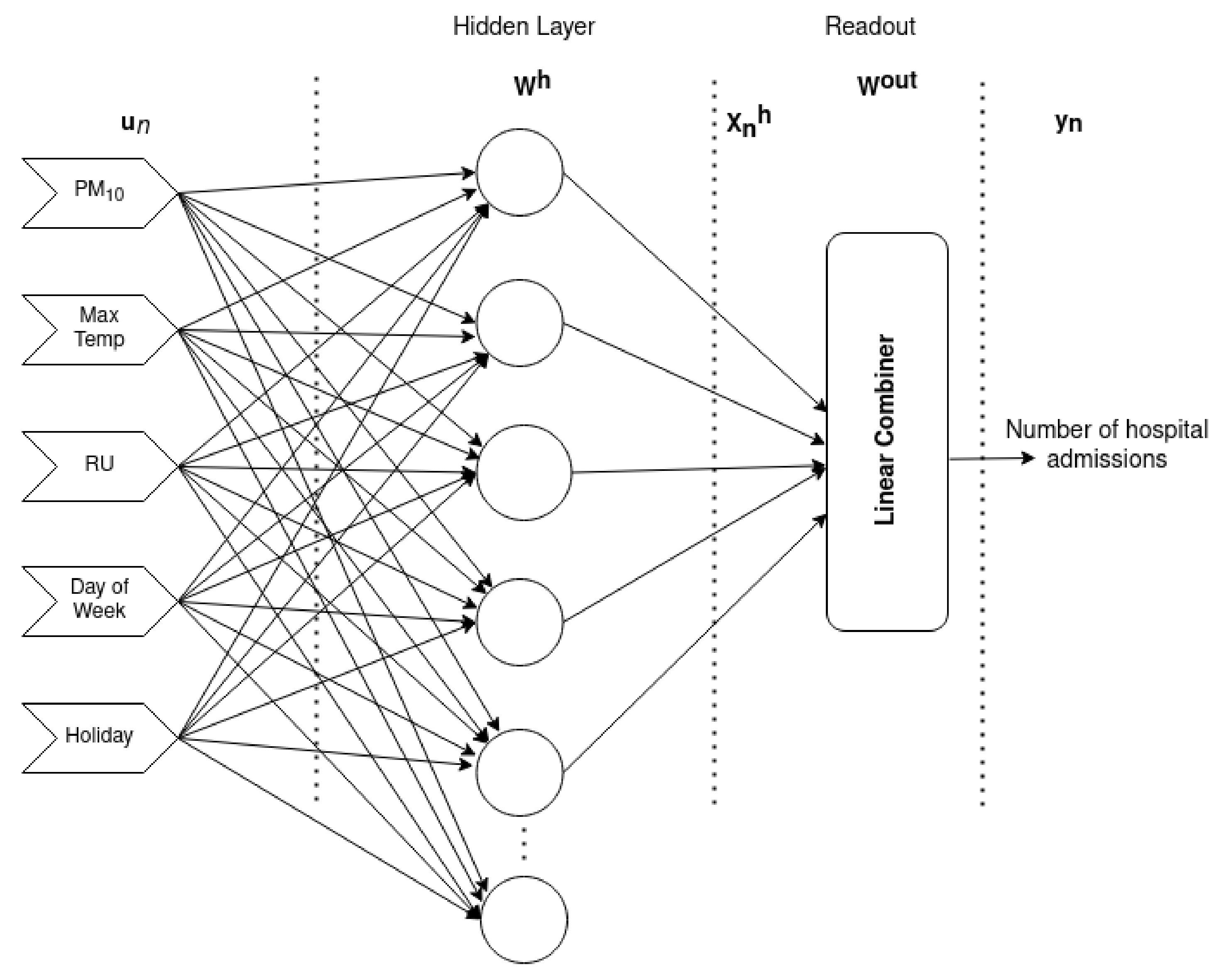
2.1. Extreme Learning Machines

The extreme learning machine (ELM) is a feedforward neural network composed of a single hidden layer, similar to the structure of multilayer perceptron (MLP) [28]. Figure 1 illustrates the architecture.
According to Figure 1, the vector u n represents all input information: PM 10 concentration; relative humidity; ambient temperature; the different weekdays; and holidays. This vector u n is associated with the matrix W h through weights of the hidden layer that can be randomly determined. The unique output layer (readout) W o u t is composed of parameters of a linear combiner that are calculated using the Moore-Penrose generalized inverse operator which shall be defined below. Finally, similar to a single-hidden layer multilayer perceptron (MLP), the ELM is also a single hidden layer feedforward neural network, being y n the output information that indicates the number of hospital admissions.
The activation of the artificial neurons within the hidden layer are given by Equation (1):
x n h = f n h ( W h u n + b ) ,
being u n = [ u n , u n 1 , , u n K 1 ] T the vector that contains the K input signals, W h R N × K the linear input coefficients, b the vector that represents the biases of the hidden units and f h ( . ) = ( f 1 h ( . ) ) , f 2 h ( . ) , , f N h ( . ) the activation functions of the hidden neurons. Then, Equation (2) presents the network outputs calculation:
y n = W o u t x n h ,
where W o u t is the output matrix.
The output layer (readout) adjustment is the main advantage of ELM models. This strategy is applied only once, considering the error signal [35,36]. Moreover, in dissonance with the traditional feedforward neural networks, when the intermediate activation functions are continuously differentiable, these models can choose the weights of the hidden layer randomly [36,37,38]. Huang et al. demonstrate that ELMs are universal approximators [39].
These structures are composed of a simple training process, mainly requiring the calculation of the parameters of a linear combiner using the Moore-Penrose generalized inverse operator, as in Equation (3) [36,37,40,41]:
W o u t = ( X h T X h ) 1 X h T d ,
where X h R T s × N is the matrix composed of the intermediate layer outputs and T s is the training sample numbers, ( X h T X h ) 1 X h T is the pseudoinverse of X h and d R T s × 1 is the vector composed of desired outputs.

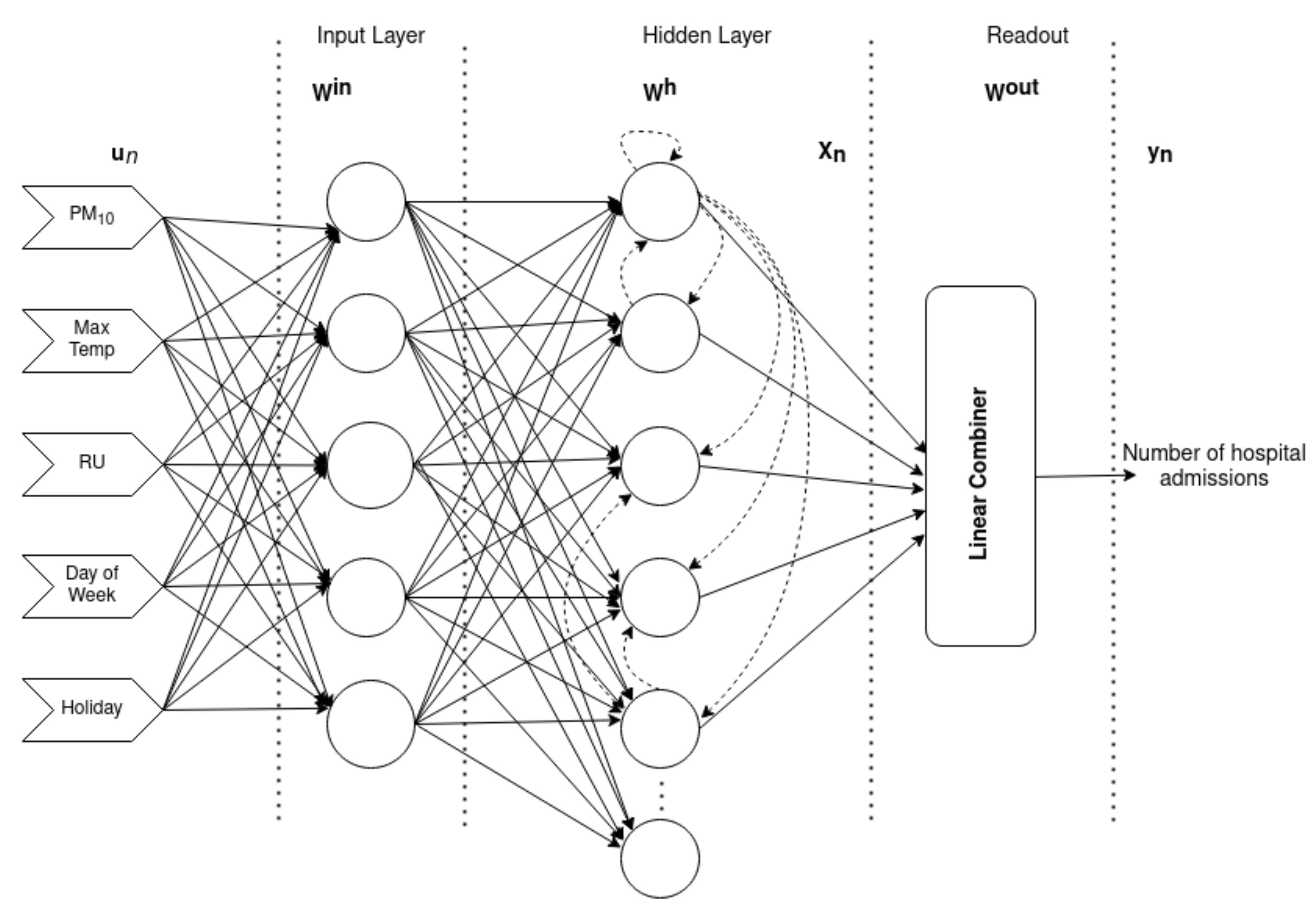
2.2. Echo State Networks

Echo state networks (ESN) are recurrent neural models known by an effortless training process: the dynamical reservoir (intermediate layer) is fixed, i.e., there is no iterative adjustment. In this sense, the synaptic weights of the reservoir do not use the error function derivatives. Thus, only the output layer is effectively adapted [42]. The adaptation process applies a linear regression scheme similar to the ELM training process, considering that a linear combiner is often applied to the output layer. The neural network structure of ESN can be seen as a general case of ELM because the reservoir presents recurrent loops. Figure 2 illustrates the structure.
Figure 2 shows that the network structure is slightly similar to the ELM model presented in Figure 1, except by the additional input layer (W i n ), defined as a linear matrix, and feedback loops in the intermediate layer (hidden layer).
Equation (4) expresses the activation of the internal neurons. This activation represents the network states which are influenced by the previous state and the present input:
x n + 1 = f ( W i n u n + 1 W x n ) ,
where f ( . ) = ( f 1 ( . ) , f 2 ( . ) , , f N ( . ) ) gives the activation functions of all neurons within the reservoir, W i n R N × K is the input weight matrix and W R N × N is the recurrent weight matrix.
The linear combinations of the reservoir signals produce the ESN outputs by (5):
y n + 1 = W o u t x n + 1 ,
where W o u t R O × N is the output weight matrix, and O the number of outputs. The parameters of the W o u t are determined by Moore-Penrose generalized inverse described in Section 2.1.
Fundamentally, the network model, besides a stable behavior, should present an internal memory that preserves the input signals history formed in the dynamical reservoir [29,35,43]. Both features are contemplated by echo state property (ESP) [29,35,43].
Jaeger et al. suggest in [29] to simplify the weight matrix W, denoting w i j as 0, 0.4 and −0.4 values with probabilities 0.95, 0.025 and 0.025, respectively. On the other hand, Ozturk et al. (2006) suggest a new design for the dynamical reservoir [44] that considers eigenvalues uniformly spreading in the weight matrix. Both approaches are applied in this work.
Having described the unorganized machines in the standard forms, the following subsections describe the variations and extensions which design structures of new models also applied to the proposed problem.

2.3. Regularization Parameter

Primarily proposed by Huang et al. (2011), the regularization strategy aims to improve the model’s generalization capability, inducing the solutions obtained by a parameter applied to the Mean Square Error (MSE) cost function. The parameter C is chosen from a validation set of samples, assuming C = 2 λ , with λ discretized in the interval [ 25 , 26 ] [32]. The strategy is performed during the interactive process, where all parameters are tested, and only one is selected according to the best MSE validation, via Expression (6):
W o u t = I C + X h T X h 1 X h T d ,
being C the regularization parameter and I the identity matrix.
Trying to improve generalization capability given by the parameter C, Kulaif et al. (2013) developed a local search, denoted golden search, to determine better values for the parameter C. The strategy is grounded in two main concepts: significant modifications are obtained in the final solutions if any small parameter variations occur; the function given by each small interval associated with the parameter C and the validation error shall be supposedly quasi-convex [45]. This strategy is also applied in this work.

2.4. Nonlinear Output Layer

Boccato et al. (2011) proposed a variation of nonlinear output layer in ESNs, the Volterra filtering structure [46]. The main concern is to prove the linear dependence between the dynamical echo states, preserving the training process simplicity for the networks. The output signals can be computed through linear combinations of polynomial terms, as in Equation (7) [27]:
y i , n = h 0 + p = 1 M h p 1 x p , n + p = 1 M q = 1 M h p , q 2 x p , n x q , n + p = 1 M q = 1 M r = 1 M h p , q , r 3 x p , n x r , n + ,
where x i , n is the output of the i t h neuron of the reservoir (or the i t h echo state) at n t h time instant, h m the linear combiner coefficient with m = 1 , , M , and M the polynomial expansion order.
Similar to Equation (3), the training process simplicity is preserved due to the linear dependence of the outputs regarding the filter parameters. In terms of least squares, Equation (7) guarantee the closed-form solution, allowing the Moore-Penrose inverse operation [47].
However, according to Boccato et al. (2011), the application of a Volterra filter might have as consequence the uncontrollable growth of free parameters and inputs numbers. To prevent these problems, a compression technique known as Principal Component Analysis (PCA) must be applied. Interestingly, the use of PCA is also suitable to avoid the redundancy between echo states [29,48]. In recent years, Chen et al. extended this idea to the ELMs, considering the same premises of the former work [48,49].
All parameters associated with the proposed models: the number of neurons, Volterra Filter orders, the weight values, and the number of simulations, shall be described in Section 4.

3. Case Studies

To evaluate the approach, three cities of São Paulo state, Brazil, with different characteristics, were considered: São Paulo, Campinas and Cubatão. The data set of daily PM 10 concentration [ μ g/m 3 ], relative humidity [%], and ambient temperature [ C], were obtained on the Environmental Sanitation Technology Company website [50].
The Brazilian National Health System provides data about the daily hospital admissions due to respiratory diseases (RD). The data set considered in this study, available in [51], comprises the International Classification of Diseases 10 (ICD-10)-J00 to J99. In this work, the database was organized as a daily format and separated by the ICD-10 diagnosis.
According to the Brazilian Institute of Geography and Statistics (IBGE) [52], São Paulo City, the largest city in Brazil, has almost 12 million people (data of 2010) in 1500 km 2 , which is 7398.26 inhabitants per km 2 . The average climate is tropical, about 28 C in summer and 12 C in winter [50]. This study considers the period from January 2014 until December 2016. The total number of hospital admissions for respiratory diseases during the studied period, for São Paulo city, was 159,683 occurrences. With regards to the PM 10 concentration, only four out of twelve air quality monitoring stations had PM 10 data. In addition, only one station presented less than 100 days of lack of data. To deal with this problem, data from another similar station were used to replace them.
Campinas City is the third most populous city of São Paulo State, with a population of approximately 1,1 million people (data of 2010) spread in 795.7 km 2 , a demographic density of 1359.6 inh/km 2 [52]. The climate is tropical with dry winter and rainy summer with an average of 37 C during summertime. For this city, the data set considered data from January 2017 to December 2019, comprising 15,464 hospital admissions for respiratory diseases. In this case, two of three air quality monitoring stations presented PM 10 data, however, one had no data for 2019. So, the only station with less missing data (145 days lack) was used.
Cubatão has an estimated 118,720 inhabitants with 142.8 km 2 and 831 inh/km 2 [52]. In the past, it was one of the most global polluted cities because of its large industrial park and for being surrounded by mountains, which makes the air dispersion hard. In the 1980s, the United Nations considered Cubatão the most polluted city in the world. After that, a government, industries and community effort controlled 98% of the air pollutants level in the city [53]. The current experiments considered the data from January 2017 to December 2019, a total of 802 hospital occurrences. For this city, all three air quality monitoring stations had PM 10 available data. However, only the station with more available data was used, with 158 missing days.
A tendency to decrease hospital admissions on the weekends and holidays is a usual situation. For this reason, the day of the week and holidays were considered as two categorical variables [54]. Thus, in addition to the PM 10 daily mean concentrations, ambient temperature (T) and relative humidity (RH), the day of the week identifications (1 for Sunday to 7 for Saturday), and a binary flag (h) to recognize if the day is a holiday, were used.
Another important feature is the lag effect of air pollution on human health [10,17,26,55]. A common practice is to consider the effect up to seven days after exposure to air pollution, where lag 0 is the effect on the same day of the exposure, and lag 7 is the effect after seven days of the exposure [54].
Table 1 presents the descriptive statistics for the target (respiratory diseases-RD) and the inputs: PM 10 concentration, temperature and relative humidity, for each city. All these variables are differed by average, standard deviation and minimum and maximum values.
Note that the cities have different patterns for the target. São Paulo hospitalizations have a wide dispersion, with 9 to 409 daily hospital admissions. Campinas ranges from 3 to 37, while Cubatão, the smallest studied city, has a maximum of eight hospitalizations. It is necessary to highlight that the databases comprise only data from the public health system, not considering data from health insurance and private units.
The maximum daily PM 10 concentration for Cubatão (148 μ g/m 3 ) draws attention, because it is almost thrice the WHO 24-hours average limit of 50 μ g/m 3 (Table 1) [56]. Despite that, the hospital admissions are very low (daily maximum of occurrences) since a significant part of the workers of Cubatão live in São Paulo, which is around 63 km far. The hospital admissions might also depend on the air pollutants dispersion pattern and the local population. São Paulo and Campinas maximum daily PM 10 concentrations are lower than Cubatão, but they are also above the WHO limit of 50 μ g/m 3 (São Paulo-maximum daily of 97 μ g/m 3 ; Campinas-maximum daily of 84 μ g/m 3 ) [56].
Since the data set described is large with high variability, it may contain multicollinearity or near-linear dependence among the variables. Multicollinearity occurs when two or more inputs (independent variables) are highly correlated affecting the estimate precision. [57]. To evaluate the data set, the Variance Inflation Factor (VIF) shall be used to diagnose the multicollinearity. VIF is calculated by an inflation of the regression coefficient for a independent variable, assessing its correlation to the dependent variables, and modeling the future relation between them. Then, the VIF for each j t h factor can be calculated as:
VIF j = 1 1 R j 2 ,
where R j 2 is the multiple determination coefficient obtained from regressing each independent variable on the others. If VIF exceeds 5, it is an indicator of multicollinearity [57].
In this work, R Studio (R version 4.1.0 (2021-05-18)—“Camp Pontanezen” Copyright (C) 2021 The R Foundation for Statistical Computing Platform: x 86 6 4 w 64 m i n g w 32 / x 64 ( 64 b i t ) ) was used to calculate VIF. The results are presented in Table 2, showing no multicollinearity between the inputs of each case study.
In the next section, the proposed models are applied to the presented data, producing a fulfilled analysis of the numerical results obtained.

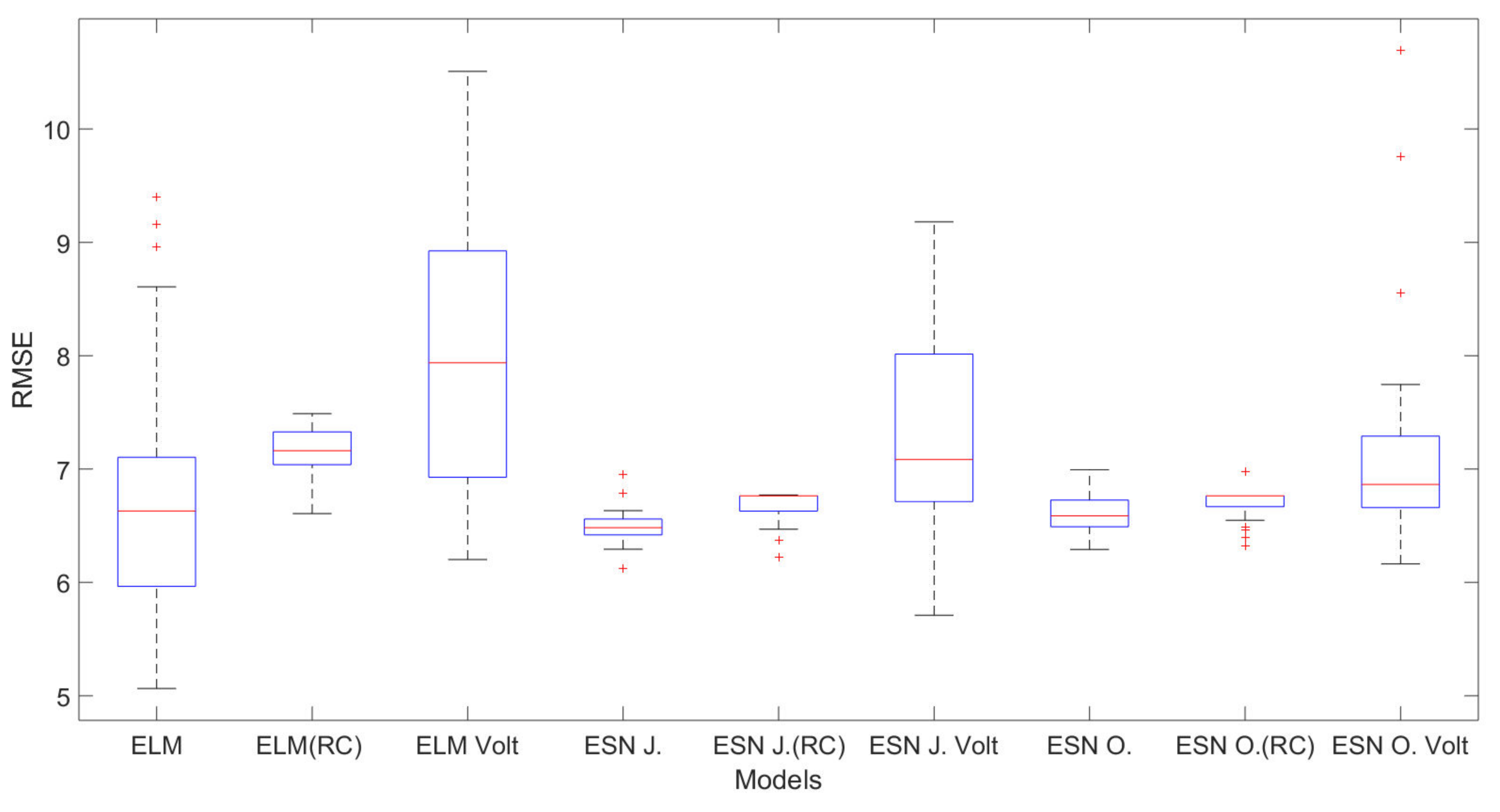
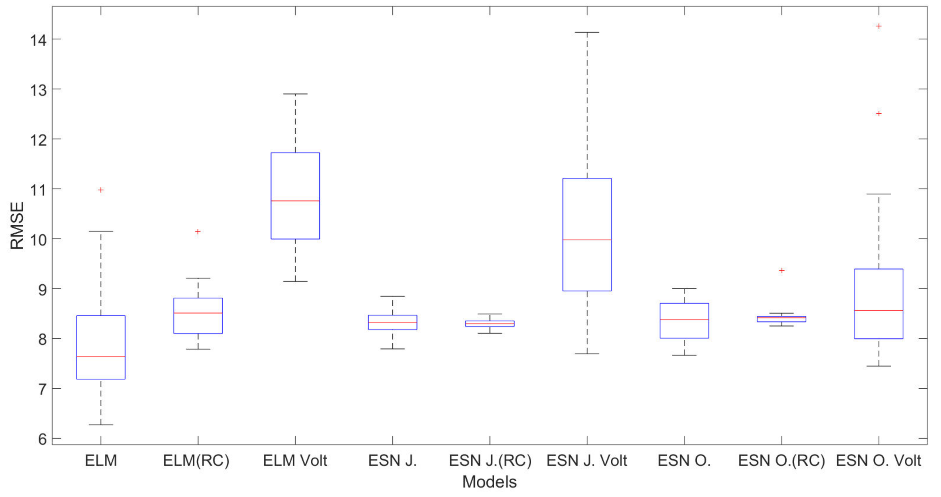
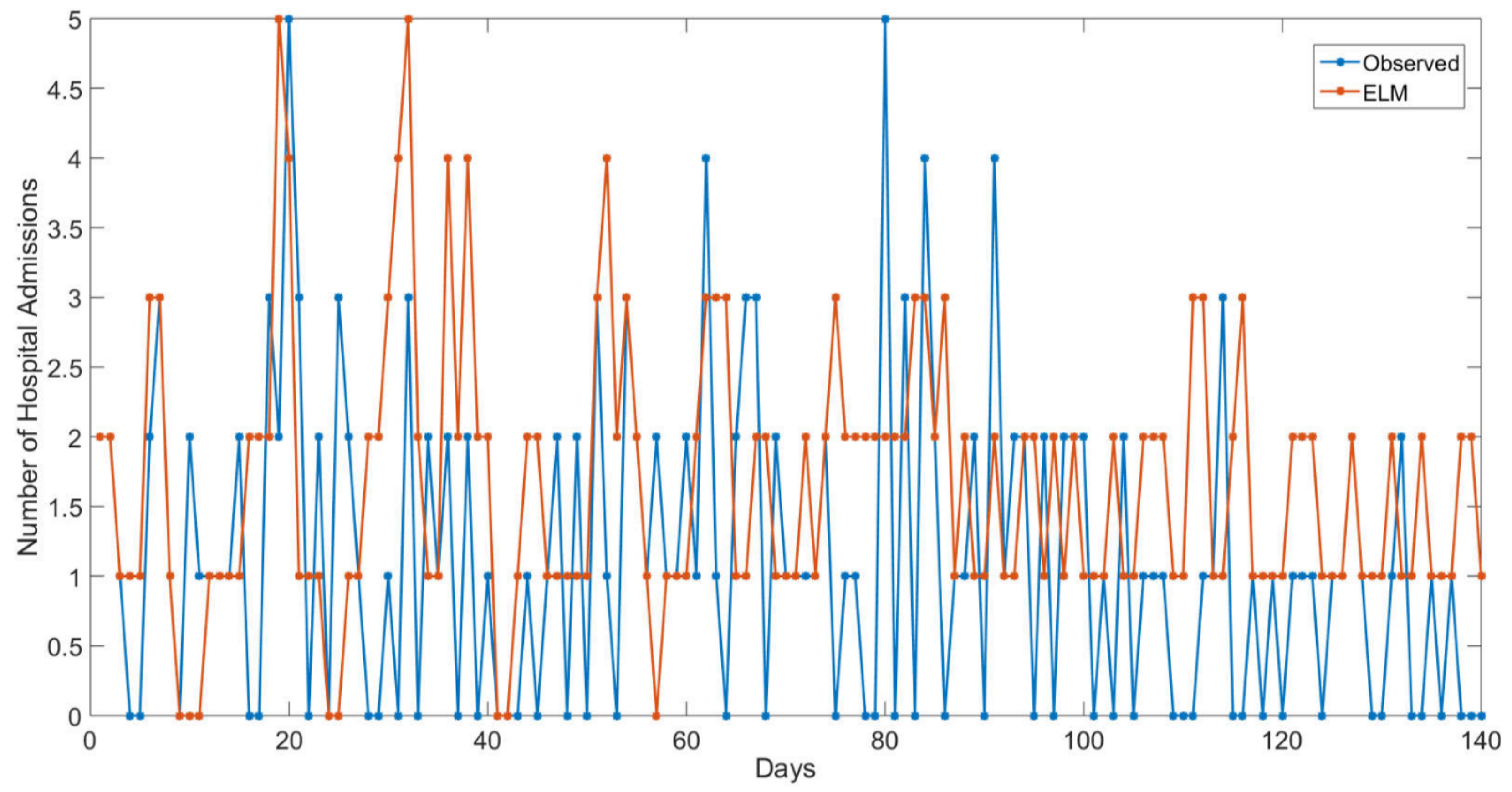
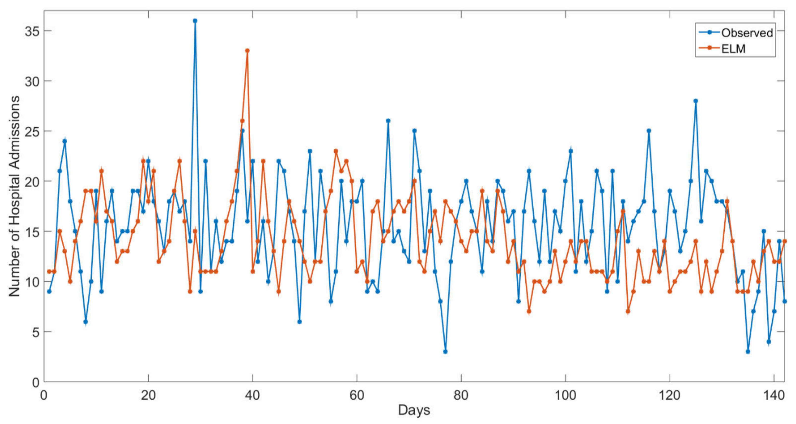
4. Results and Critical Analysis

The following items describe all models developed to obtain the numerical results in order to evaluate the approach’s effectiveness:
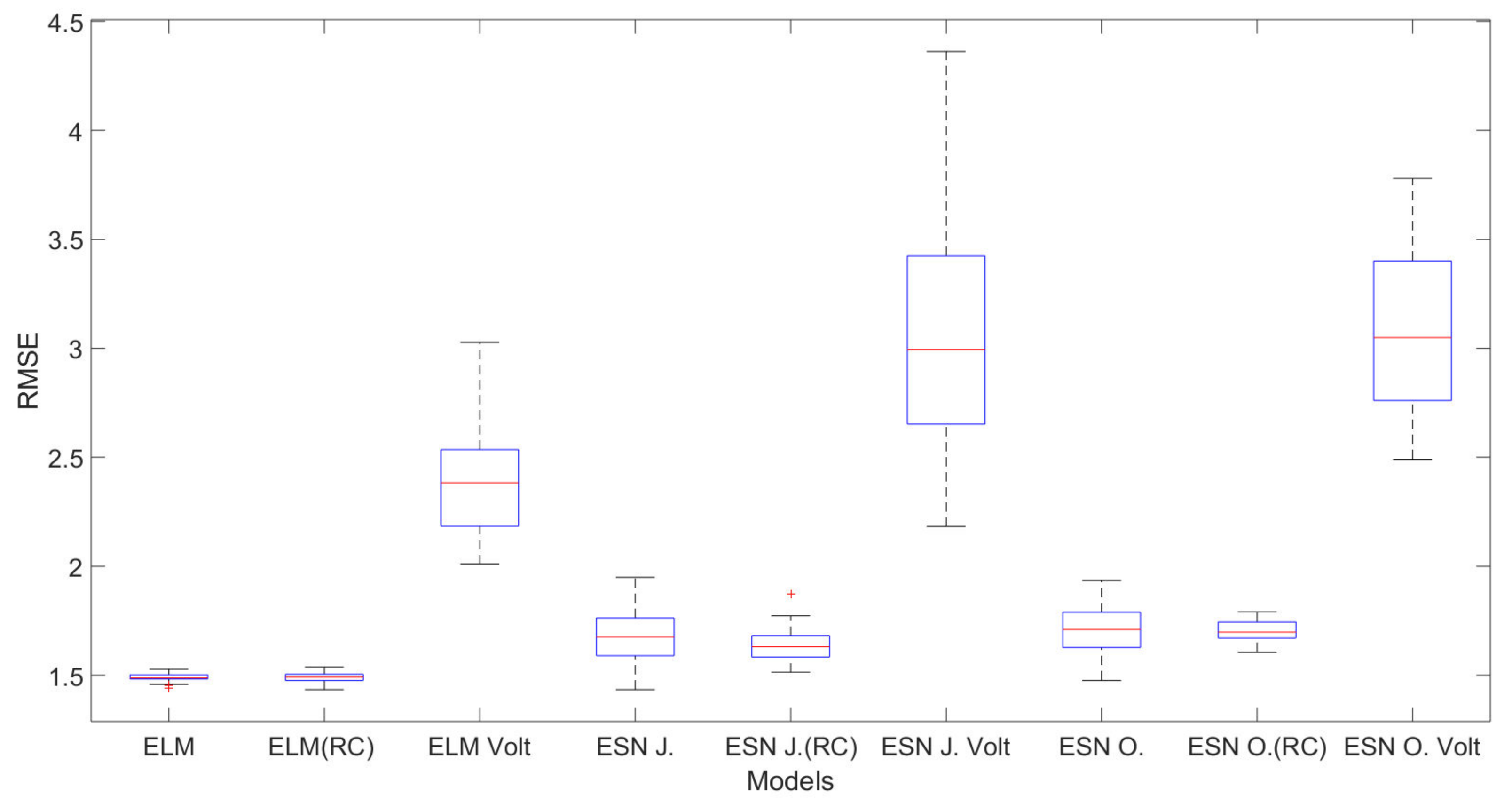
  • Standard single models: Three versions are developed considering the Standard Models presented in Section 2.1 and Section 2.2. The Extreme Learning Machine (ELM), the Echo State Network from Jaeger et al. [29] (ESN J.) and the Echo State Network from Ozturk et al. [44] (ESN O.);
  • Regularization Parameter: All standard models are extended, producing three other models through regularization parameter concepts presented in Section 2.3. The ELM with Regularization Parameter (ELM–RP), the ESN J. with Regularization Parameter (ESN J.–RP) and the ESN O. with Regularization Parameter (ESN O.–RP);
  • Nonlinear Output Layers: Similarly, three more models are proposed considering the concepts in Section 2.4. The Nonlinear Output Layers strategy is applied to the three single forms creating the ELM with Volterra Filtering Structure (ELM Volt), the ESN J. with Volterra Filtering Structure (ESN J. Volt), and the ESN O. with Volterra Filtering Structure (ESN O. Volt).
The experimental procedure follows the steps summarized in Figure 3:
The process begins by collecting the data in the mentioned repositories. Before the insertion of the samples in the neural networks, a normalization procedure is performed due to the limits of the activation function saturation [58]. After the training samples are inserted in the model in order to adjust their free parameters, observing the decrease of the output error. During this process, cross-validation is performed to increase the system generalization capability.
When the training ends, the test samples are inserted in the ANN after the input normalization. The neural response is stored, the normalization is reversed and, finally, the model output is available, which allows the calculation of the models’ error. In this work, all models codes were developed in the MATLAB language.
In the training step, the parameters were defined as follows:
  • The number of artificial neurons in the hidden layer (or dynamic reservoir) of each model was determined considering a grid search ranging from 3 to 450 neurons;
  • The weights were randomly generated in the interval [ 1 ; + 1 ] ;
  • The hyperbolic tangent was addressed as the activation function of the hidden layers;
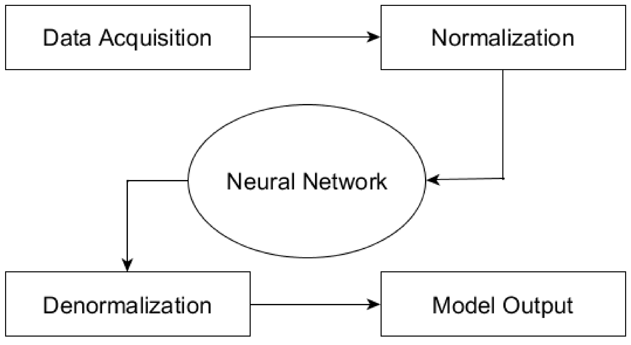
  • The samples were normalized in the interval [ 1 ; + 1 ] before the neural processing;
  • The models with RP strategy considered the holdout cross-validation;
  • The reservoir designed by Ozturk et al. considered a spectral radius of 0.95 [44];
  • The first and the third orders (Equation (7)) of the Volterra filter and the first three principal components of the PCA were considered [48]. These values were defined after empirical tests;
  • Before the calculation of the errors, the original domain data was re-scaled.
This work addressed three error metrics to evaluate the solutions quality: Root Mean Square Error (RMSE), Mean Absolute Error (MAE), and Mean Absolute Percentage Error (MAPE), given by (9)–(11), respectively:
RMSE = 1 N n = 1 N ( d n y n ) 2 ,
MAE = 1 N n = 1 N | d n y n | ,
MAPE = 1 N n = 1 N d n y n d n × 100 ,
where d n is the actual value, y n is the neural model response and N is the total number of samples.
Table 3, Table 4 and Table 5 present the computational performances achieved by the nine proposed models for each lag, considering each city. The results present the number of neurons (NN) used in the best performance and the error metrics: RMSE, MAE and MAPE. However, as it can be seen in Table 3 for Cubatão, the error metrics MAPE was not considered due to the expressive number of “zeros” for the actual value ( d n ). In the tables, the best results obtained for each error metric and the best model are highlighted in purple. Furthermore, the models highlighted in italic bold with stars are the models which obtained statistically similar results to the best one. This statistical test is described below.
A specific result analysis shows that ELM(RP) had the best results for the all calculated metrics for Cubatão in lag 2. Besides, ELM obtained the best results for Campinas, considering the error metrics RMSE and MAPE in lag 3, but for MAE, ELM(RP) achieved the best results in lag 0. For São Paulo, ELM obtained the smallest error values for different lags: RMSE in lag 2 and MAE in lag 1. Finally, ELM(RP) presented the smallest error metric MAPE in lag3.
Note that the best results obtained by the models sometimes were not replicated for all error metrics. This behavior was evident for São Paulo and Campinas, since the best lag and the best model were not always the same. Similar behavior can be observed in [17,59].
The pairwise Wilcoxon test was applied to evaluate if the results are statistically different considering the RMSE with 30 independent simulations [60]. In Table 3 and Table 4, the models highlighted in bold with star tag achieved a p-value higher than 0.05, which means that there is no statistical difference between their results and the best one. For this reason, these models can be considered similar, in terms of performance, to the models that obtained the best results. For Campinas, the standard ELM and all ESNs presented equivalent performances, despite the numerical values being contrasts. For Cubatão, ELM and ELM(RP) results were also similar. At long last, for São Paulo the test did not show any statistical similarity among the models.
Figure 4, Figure 5 and Figure 6 show the boxplot graphic regarding the RMSE values for each city and the lag associated with the best result.
Considering Cubatão, observe that the smallest dispersion was obtained by ELM (RP) model, which also presented the smallest average value, corroborating the observation from Table 3. The inclusion of the Volterra filter increases the dispersion and the average values for all standard models, representing a significant degree of deterioration in performance.
In Campinas’ case, only the ELM performances will be considered in this specific analysis since all ESN obtained similar results according to the Wilcoxon test. However, Figure 5 illustrates all models to avoid any curiosity. The RP inclusion decreases the dispersion, while the Volterra filter showed an opposite behavior. Despite that, the best performance in terms of best results regarding 30 simulations was favorable to the use of Volterra filter instead of the RP (note the bottom value in the boxplot). Since the generation of the neurons’ weights were random, the algorithms must run at least 30 times, and this fact directly implied a long tail for the boxplots, as can be seen in the Volterra models. Moreover, the best result obtained by ELM does not mean the best performance in terms of dispersion.
For São Paulo, the general behavior of the standard models was similar to Campinas. The standard ELM achieved better general errors, even when considered the median value. The inclusion of the RP reduced the dispersion, but it decreased the probability of obtaining better results for the error metrics. On the other hand, the Volterra filter showed a worse performance in terms of dispersion. However, despite the ELM best results for error metric, the model presented a bad dispersion, including an outlier.
Table 6 presents a ranking of best error metric results considering all neural models in ascending order of development. Note that the draws regarding the winners mean that there was no statistical difference between the models. The last column represents the final ranking considering the three cities’ results.
The standard ELM was the best estimator in all cases as regards the error metric results, but for Cubatão, the results obtained by ELM(RP) were the same. The second and third positions show ESN O. and ESN J. models, respectively. However, despite the main contribution of RP is to increase the models’ generalization capability, its use reduced the dispersion of the results, i.e., the models’ predictability increased, except for Cubatão. Moreover, the ELM(RP) ranking position was deteriorated by the Campinas results, since all ESNs presented the same statistical performance. Dismissing these aspects, the model could be the second best.
Although the inclusion of the Volterra filter did not improve the performances, the idea of its application was to capture nonlinear patterns among the signals from the hidden layer. Despite the literature presents good performances for this method in correlated tasks [33], its use is not recommended in this case. Similarly, the inclusion of the reservoir designed by Jaeger or Ozturk et al. is not adequate to the problem.
Regarding the number of neurons in the hidden layers (dynamic reservoir), one can see miscellaneous neurons, with a high degree of variation. For Cubatão, the pattern noted was the models used hundreds of neurons in most cases. Interestingly, ESN J. and ESN O. often addressed up to 70 neurons. Moreover, it can be seen in Campinas’ case, that the RP models used up to 35 neurons in all cases. Considering São Paulo, the ELM versions tended to use less than 25 neurons, similar to ESN J. Volt, ESN O. and ESN O. Volt. The others models addressed hundreds of neurons. This is a strong indication that a sweep in the neuron amount is needed because a clear pattern regarding this parameter was not found. Even considering the results of the models that presented a p-value large than 0.05, the number of neurons was variable.
In summary, the unorganized machines are particular cases of classic neural models, which the hidden weights are not adjusted. On one hand, the user may lose part of the approximation capability due to this characteristic; on the other hand, there are gains in terms of training effort and stability for the output values during the training, avoiding discrepancies. An important aspect is that these methodologies can be outperformed, depending on the problem. Regarding the use of RP or Volterra filter, the literature indicates that these strategies may increase the mapping capability of the neural models. However, this work showed that in specific cases these approaches did not present efficiency.
Figure 7, Figure 8 and Figure 9 present the best evolution of the output response in comparison to the actual values.
Figure 7 shows that the prediction task seems to be more difficult when the output has a small range and many “zero” observations. In this case, as the overestimation was small, given that the observed values are zero, it did not interfere in hospital management. Otherwise, in Figure 8, since there were no “zero” observations, the ELM estimations could be considered a suitable performance, except in abrupt cases.
Finally, in Figure 9, ELM reached the smallest RMSE, but comparing with the observed data, it was more difficult to predict the abrupt decrease of hospital admissions occurred around day 70. On the other hand, the ELM(RP) could follow this tendency, but it over and underestimated the number of hospital admissions in many cases. These behaviors are directly related to the number of neurons used by each model since a reduction in this number limited the model approximation capability.
Regarding the best error metric to be used, RMSE seems to be a good strategy, since the error metric was reduced during the neural models training (adjustment) [17,18,61].
Table 7 presents a summary of some notable studies showing the association between air pollutants concentration, morbidity (Hospital Admissions or Hospital Emergency) and mortality. This brief description relates the authors, geographic area, considered inputs and predicted variables, the applied methods, metrics, time base, and the best MAPE and RMSE observed for each study. Although these studies present suitable estimations and relevant contributions, they proposed different models, and applied to diverse worldwide places, using specific inputs to predict health effects. For this reason, a comparative analysis of these studies’ performances is unfair, as Katri and Tamil [62] previously observed. However, some important aspects can be highlighted.
Two studies [62,63] did not use MAPE or RMSE as error metrics. Khatri and Tamil [62] aimed to compare the performance for peak and non-peak class prediction. The authors used percentage difference in this study and applied MLP, without any consideration about other methods’ performance. Shakerkhatibi et al. [64] used other metrics (Delong Method) to compare the predictions using MLP and Conditional Logistic Regression.
Table 7. Summary of studies presenting air pollutant’s associations with morbidity and mortality using ANN.
Authors (Year)Geographic Area of StudyInputsPredicted VariableMethodsUsed MetricsTime BaseBest MAPEBest RMSE
Kassomenos et al. (2011) [24]AthensT, RH, WD, SO 2 , black smoke
CO, NO 2 , NO, O 3
HA for Cardiorespiratory diseasesMLP, GLMRMSEdailyNA0.8950
Moustris et al. (2012) [63]AthensT, RH, WS, solar radiation
SO 2 , PM 10 , CO, O 3 , NO 2
(age subgroups
0–4 years, 5–14 years, 0–14 years)
HA for AsthmaMLP (TLRN)MBE, RMSE,
R 2 , IA
dailyNA3.2
Cengiz and Terzi (2012) [65]Afyon, TurkeySO 2 , PM 10 HA and symptoms
(cough, exertional, dyspnea, expectoration)
for COPD
MLP, RBF, GLM, GAMRMSE e MAPEweekly4.542.38
Shakerkhatibi et al. (2015) [64]Tabriz, IranT, RH, NO, NO 2 , NO X , SO 2 , CO, PM 10 , O 3
(age and gender subgroups)
HA for respiratory and cardiovascular diseasesMLP, CLRAUC, sensitivity, Specificity and Accuracy (%)dailyNANA
Khatri and Tamil (2017) [62]Dallas County, Texas, USAT, RH, WS, CO, O 3 , SO 2 , NO 2 , PM 2.5 HE for respiratory diseasesMLP% differencedailyNANA
Tadano et al. (2016) [26]Campinas city, São Paulo state, BrazilT, RH, PM 10 HA for respiratory diseasesMLP, ESN, ELMMSE/MAPEdaily31.25.98
Polezer et al. (2018) [10]Curitiba, Paraná, BrazilT, RH, PM 2.5 HA for respiratory diseasesMLP, ESN, ELMMSE/MAPEdaily29.877.37
Araujo et al. (2020) [17]Campinas and São Paulo cities, BrazilT, RH, PM 10 HA for respiratory diseasesMLP, GLM, ELM, ESN, RBF, EnsembleMSE, MAE, MAPEdaily24.873.04
Zhou, Li and Wang (2018) [66]Hangzhou, Southern part of the Yangtze River Delta, ChinaT, PM 10 , PM 2.5 , NO 2 , SO 2 Respiratory disease casesMLP, GAMAIC, MSEdailyNA2.17
Kachba et al. (2020) [18]São Paulo city, BrazilCO, NO x , O 3 , SO 2 , PMHA and mortality for respiratory diseasesMLP, ELM, ESNMSE, MAE, MAPEmonthly34.53160.26
WD-Wind Direction; WS-Wind Speed; SO 2 -Sulphur Dioxide; CO-Carbon Monoxide; NO 2 -Nitrogen Dioxide; NO-Nitrogen Monoxide; O 3 -Ozone; NO x -Nitrogen Oxides; HE-Hospital Emergency; GAM-Generalized Additive Models; TLRN-Time Lagged Recurrent Networks; RBF-Radial Basis Function Network; CLR-Conditional Logistic Regression Modeling; MBE-Mean Bias Error; IA-Index of Agreement; AUC-area under curve.
Considering the variety of applied methods (Table 7), and emphasizing the use of MLP, the performance comparison between ANN and regression models has proved the ANN superior performance. Inspired by these all aspects, the paper’s authors believe that this present work, which explores the ELM and ESN models with variations from the RP and the Volterra filter to estimate hospital admissions due to respiratory diseases caused by air pollutants concentration, is a relevant contribution. However, given the harmful effects of PM on human health, and comparing the considered input variables used in the other studies, this work has some limitations, such as the use of only one air pollutant (PM 10 ) and the lack of comparison with a statistical regression modeling.

5. Conclusions

This work predicted the hospital admissions due to respiratory diseases caused by the particulate matter PM 10 concentrations using the extreme learning machines (ELM) and the echo state networks (ESN) in the standard forms and applying the variations from the regularization parameter (RP) and the Volterra filter. The estimates considered daily PM 10 concentration, relative humidity, ambient temperature as inputs and predicted the daily hospital admissions for respiratory diseases.
Numerical results indicated the superior performance of the standard models, pointing to ELM as the best predictor for most scenarios. However, regarding Campinas city and the RMSE error metric, a statistical test demonstrated that ESN models were statistically similar when compared to the best one. Besides, a graphic analysis showed that the models with the inclusion of RP strategy presented a reduced dispersion, considering the abrupt variations in hospital admissions, while the Volterra filter showed an opposite behavior, indicating that its application was not suitable for this specific problem. Finally, completing the critical analysis, a ranking of performances classified the models regarding the error metrics for each city. This ranking rewarded the models with statistical similarity rather than models with good dispersion, highlighting the standard models in the first positions.
The application of Unorganized Machines to three different cities was essential to evaluate their good performance in predicting air pollution impacts on human health. An additional graphic analysis of the output response in comparison to the actual values, for the best models, evidenced the good performance of the neural networks to estimate the hospital admissions. This contribution may help governmental bodies and policymakers on the management of hospital planning, mainly during air pollution unfavorable climate periods. Moreover, the good performance of the models confirms the link between all input variables and the output values, verifying that the particulate matter, temperature and relative humidity are fundamental to obtain a good estimation.
A limitation of this study is the lack of large data sets that could bring more uniform performances between the studied cities. As a consequence of the lack of monitoring data, other pollutants variations such as PM 2.5 cannot be studied.
Considering the continental dimension of Brazil and the characteristics of the different region’s climates, it would be paramount to study all regions (states), a hard task due to the lack of monitoring all over the country. Further works shall consider hybrid modeling or ensembles, the use of deseasonalization techniques, and the appliance of other artificial neural networks. Since the ELM is admittedly susceptible to the neurons number changes in the hidden layer and the ESN model is considered robust in this regard, a comparison study should be conducted pointing to the training time required between these models.

Author Contributions

Conceptualization, Y.d.S.T., E.T.B., L.C., and H.V.S.; methodology, H.V.S. and Y.d.S.T.; software, H.V.S., T.S.P., E.P., and T.A.A.; formal analysis, Y.d.S.T., E.T.B., and L.C.; investigation, H.V.S., E.P., T.A.A., and Y.d.S.T.; resources, H.V.S.; data curation, E.T.B. and L.C.; writing—original draft preparation, E.T.B., L.C., and H.V.S.; writing—review and editing, Y.d.S.T. and C.M.L.U.; visualization, H.V.S. and T.A.A.; supervision, Y.d.S.T. and H.V.S.; project administration, H.V.S.; funding acquisition, H.V.S. All authors have read and agreed to the published version of the manuscript.

Funding

This research was funded by the National Council for Scientific and Technological Development (CNPq), grant number 405580/2018-5, and the APC was funded by DIRPPG/UTFPR/PG.

Acknowledgments

The authors thank the Brazilian agencies Coordination for the Improvement of Higher Education Personnel (CAPES)-Financing Code 001, Brazilian National Council for Scientific and Technological Development (CNPq), processes number 40558/2018-5, 315298/2020-0, and Araucaria Foundation, process number 51497, and Federal University of Technology-Parana (UTFPR) for their financial support.

Conflicts of Interest

The authors declare no conflict of interest.

References

  1. WHO-World Health Organization. Ambient Air Pollution: Health Impacts; WHO: Geneva, Switzerland, 2018. [Google Scholar]
  2. Lelieveld, J.; Evans, J.S.; Fnais, M.; Giannadaki, D.; Pozzer, A. The contribution of outdoor air pollution sources to premature mortality on a global scale. Nature 2015, 525, 367. [Google Scholar] [CrossRef] [PubMed]
  3. Manisalidis, I.; Stavropoulou, E.; Stavropoulos, A.; Bezirtzoglou, E. Environmental and health impacts of air pollution: A review. Front. Public Health 2020, 8, 14. [Google Scholar] [CrossRef] [PubMed] [Green Version]
  4. Li, X.; Liu, X. Effects of PM2.5 on chronic airway diesases: A review of research progress. Atmosphere 2021, 12, 1068. [Google Scholar] [CrossRef]
  5. Ab Manan, N.; Aizuddin, A.N.; Hod, R. Effect of air pollution and hospital admission: A systematic review. Ann. Glob. Health 2018, 84, 670. [Google Scholar] [CrossRef] [PubMed] [Green Version]
  6. Grigorieva, E.; Lukyanets, A. Combined effect of hot weather and outdoor air pollution on respiratory health: Literature review. Atmosphere 2021, 12, 790. [Google Scholar] [CrossRef]
  7. Morrissey, K.; Chung, I.; Morse, A.; Parthasarath, S.; Roebuck, M.M.; Tan, M.P.; Wood, A.; Wong, P.F.; Forstick, S.P. The effects of air quality on hospital admissions for chronic respiratory diseases in Petaling Jaya, Malaysia, 2013–2015. Atmosphere 2021, 12, 1060. [Google Scholar] [CrossRef]
  8. Yitshak-Sade, M.; Nethery, R.; Schwartz, J.D.; Mealli, F.; Dominici, F.; Di, Q.; Awad, Y.A.; Ifergane, G.; Zanobetti, A. PM2.5 and hospital admissions among Medicare enrollees with chronic debilitating brain disorders. Sci. Total Environ. 2021, 755, 142524. [Google Scholar] [CrossRef]
  9. Anderson, J.O.; Thundiyil, J.G.; Stolbach, A. Clearing the air: A review of the effects of particulate matter air pollution on human health. J. Med. Toxicol. 2012, 8, 166–175. [Google Scholar] [CrossRef] [Green Version]
  10. Polezer, G.; Tadano, Y.S.; Siqueira, H.V.; Godoi, A.F.; Yamamoto, C.I.; de André, P.A.; Pauliquevis, T.; de Fatima Andrade, M.; Oliveira, A.; Saldiva, P.H.; et al. Assessing the impact of PM 2.5 on respiratory disease using artificial neural networks. Environ. Pollut. 2018, 235, 394–403. [Google Scholar] [CrossRef]
  11. Ardiles, L.G.; Tadano, Y.S.; Costa, S.; Urbina, V.; Capucim, M.N.; da Silva, I.; Braga, A.; Martins, J.A.; Martins, L.D. Negative binomial regression model for analysis of the relationship between hospitalization and air pollution. Atmos. Pollut. Res. 2018, 9, 333–341. [Google Scholar] [CrossRef]
  12. McCullagh, P.; Nelder, J.A. Generalized Linear Models; Routledge: London, UK, 2019. [Google Scholar]
  13. Belotti, J.T.; Castanho, D.S.; Araujo, L.N.; da Silva, L.V.; Alves, T.A.; Tadano, Y.S.; Stevan, S.L., Jr.; Correa, F.C.; Siqueira, H.V. Air Pollution Epidemiology: A Simplified Generalized Linear Model Approach Optimized by Bio-Inspired Metaheuristics. Environ. Res. 2020, 191, 110106. [Google Scholar] [CrossRef] [PubMed]
  14. Cromar, K.; Galdson, L.; Palomera, M.J.; Perlmutt, L. Development of a health-based index to indentify the association between air pollution and health effects in Mexico City. Atmosphere 2021, 12, 372. [Google Scholar] [CrossRef]
  15. Ravindra, K.; Rattan, P.; Mor, S.; Aggarwal, A.N. Generalized additive models: Building evidence of air pollution, climate change and human health. Environ. Int. 2019, 132, 104987. [Google Scholar] [CrossRef] [PubMed]
  16. Zhou, H.; Geng, H.; Dong, C.; Bai, T. The short-term harvesting effects of ambient particulate matter on mortality in Taiyuan elderly residents: A time-series analysis with a generalized additive distributed lag model. Ecotoxicol. Environ. Saf. 2021, 207, 111235. [Google Scholar] [CrossRef]
  17. Araujo, L.N.; Belotti, J.T.; Antonini Alves, T.; de Souza Tadano, Y.; Siqueira, H. Ensemble method based on Artificial Neural Networks to estimate air pollution health risks. Environ. Model. Softw. 2020, 123, 104567. [Google Scholar] [CrossRef]
  18. Kachba, Y.; Chiroli, D.M.d.G.; Belotti, J.T.; Antonini Alves, T.; de Souza Tadano, Y.; Siqueira, H. Artificial Neural Networks to Estimate the Influence of Vehicular Emission Variables on Morbidity and Mortality in the Largest Metropolis in South America. Sustainability 2020, 12, 2621. [Google Scholar] [CrossRef] [Green Version]
  19. Cabaneros, S.M.; Calautit, J.K.; Hughes, B.R. A review of artificial neural network models for ambient air pollution prediction. Environ. Model. Softw. 2019, 119, 285–304. [Google Scholar] [CrossRef]
  20. de Mattos Neto, P.S.; Madeiro, F.; Ferreira, T.A.; Cavalcanti, G.D. Hybrid intelligent system for air quality forecasting using phase adjustment. Eng. Appl. Artif. Intell. 2014, 32, 185–191. [Google Scholar] [CrossRef]
  21. Feng, R.; Zheng, H.J.; Gao, H.; Zhang, A.R.; Huang, C.; Zhang, J.X.; Luo, K.; Fan, J.R. Recurrent Neural Network and random forest for analysis and accurate forecast of atmospheric pollutants: A case study in Hangzhou, China. J. Clean. Prod. 2019, 231, 1005–1015. [Google Scholar] [CrossRef]
  22. Neto, P.S.D.M.; Firmino, P.R.A.; Siqueira, H.; Tadano, Y.D.S.; Alves, T.A.; De Oliveira, J.F.L.; Marinho, M.H.D.N.; Madeiro, F. Neural-Based Ensembles for Particulate Matter Forecasting. IEEE Access. 2021, 9, 14470–14490. [Google Scholar] [CrossRef]
  23. Wang, Q.; Liu, Y.; Pan, X. Atmosphere pollutants and mortality rate of respiratory diseases in Beijing. Sci. Total Environ. 2008, 391, 143–148. [Google Scholar] [CrossRef]
  24. Kassomenos, P.; Petrakis, M.; Sarigiannis, D.; Gotti, A.; Karakitsios, S. Identifying the contribution of physical and chemical stressors to the daily number of hospital admissions implementing an artificial neural network model. Air Qual. Atmos. Health 2011, 4, 263–272. [Google Scholar] [CrossRef]
  25. Sundaram, N.M.; Sivanandam, S.; Subha, R. Elman neural network mortality predictor for prediction of mortality due to pollution. Int. J. Appl. Eng. Res 2016, 11, 1835–1840. [Google Scholar]
  26. Tadano, Y.S.; Siqueira, H.V.; Antonini Alves, T. Unorganized machines to predict hospital admissions for respiratory diseases. In Proceedings of the IEEE Latin American Conference on Computational Intelligence (LA-CCI), Cartagena, Colombia, 2–4 November 2016; pp. 1–6. [Google Scholar]
  27. Boccato, L.; Soares, E.S.; Fernandes, M.M.L.P.; Soriano, D.C.; Attux, R. Unorganized Machines: From Turing’s Ideas to Modern Connectionist Approaches. Int. J. Nat. Comput. Res. (IJNCR) 2011, 2, 1–16. [Google Scholar] [CrossRef] [Green Version]
  28. Huang, G.; Huang, G.B.; Song, S.; You, K. Trends in extreme learning machines: A review. Neural Netw. 2015, 61, 32–48. [Google Scholar] [CrossRef] [PubMed]
  29. Jaeger, H. The “echo state” approach to analysing and training recurrent neural networks-with an erratum note. Bonn, Ger. Ger. Natl. Res. Cent. Inf. Technol. GMD Tech. Rep. 2001, 148, 13. [Google Scholar]
  30. Jaeger, H. Short term memory in Echo State Networks; Technical Report; Fraunhofer Institute for Autonomous Intelligent Systems: Sankt Augustin, Germany, 2001. [Google Scholar]
  31. Siqueira, H.V.; Boccato, L.; Attux, R.; Lyra Filho, C. Echo state networks in seasonal streamflow series prediction. Learn. Nonlinear Model. 2012, 10, 181–191. [Google Scholar] [CrossRef] [Green Version]
  32. Huang, G.B.; Zhou, H.; Ding, X.; Zhang, R. Extreme learning machine for regression and multiclass classification. IEEE Trans. Syst. Man, Cybern. Part B Cybern. 2011, 42, 513–529. [Google Scholar] [CrossRef] [Green Version]
  33. Boccato, L.; Lopes, A.; Attux, R.; Von Zuben, F.J. An extended echo state network using Volterra filtering and principal component analysis. Neural Networks Off. J. Int. Neural Netw. Soc. 2012, 32, 292–302. [Google Scholar] [CrossRef]
  34. Butcher, J.; Verstraeten, D.; Schrauwen, B.; Day, C.; Haycock, P. Extending reservoir computing with random static projections: A hybrid between extreme learning and RC. In Proceedings of the 18th European sSymposium on Artificial Neural Networks, Bruges, Belgium, 28–30 April 2010. [Google Scholar]
  35. Yildiz, I.B.; Jaeger, H.; Kiebel, S. Re-visiting the echo state property. Neural Netw. 2012, 35, 1–9. [Google Scholar] [CrossRef]
  36. Huang, G.B.; Zhu, Q.Y.; Siew, C.K. Extreme learning machine: Theory and applications. Neurocomputing 2006, 70, 489–501. [Google Scholar] [CrossRef]
  37. Huang, G.; Chen, L.; Siew, C. Universal approximation using incremental constructive feedforward networks with random hidden nodes. IEEE Trans. Neural Netw. 2006, 17, 879–892. [Google Scholar] [CrossRef] [Green Version]
  38. Cao, J.; Lin, Z.; Huang, G.B.; Liu, N. Voting based extreme learning machine. Inf. Sci. 2012, 185, 66–77. [Google Scholar] [CrossRef]
  39. Siqueira, H.; Luna, I. Performance comparison of feedforward neural networks applied to streamflow series forecasting. Math. Eng. Sci. Aerosp. (MESA) 2019, 10, 41–53. [Google Scholar]
  40. Bartlett, P. The Sample Complexity of Pattern Classification with Neural Networks: The Size of the Weights is More Important than the Size of the Network. IEEE Trans. Inf. Theory 1998, 44, 525–536. [Google Scholar] [CrossRef] [Green Version]
  41. Liu, X.; Gao, C.; Li, P. A comparative analysis of support vector machines and extreme learning machines. Neural Netw. 2012, 33, 58–66. [Google Scholar] [CrossRef] [PubMed]
  42. Siqueira, H.; Boccato, L.; Attux, R.; Lyra, C. Echo state networks and extreme learning machines: A comparative study on seasonal streamflow series prediction. In Proceedings of the International Conference on Neural Information Processing, Doha, Qatar, 12–15 November 2012; pp. 491–500. [Google Scholar]
  43. Lukosevicius, M.; Jaeger, H. Reservoir computing approaches to recurrent neural network training. Comput. Sci. Rev. 2009, 3, 127–149. [Google Scholar] [CrossRef]
  44. Ozturk, M.C.; Xu, D.; Príncipe, J.C. Analysis and design of Echo State Networks. Neural Comput. 2007, 19, 111–138. [Google Scholar] [CrossRef]
  45. Kulaif, A.C.P.; Von Zuben, F.J. Improved regularization in extreme learning machines. In Proceedings of the 11th Brazilian Congress on Computational Intelligence Porto de Galinhas, Pernambuco, Brazil, 8–11 September 2013; Volume 1, pp. 1–6. [Google Scholar]
  46. Hashem, S. Optimal linear combinations of neural networks. Neural Netw. 1997, 10, 599–614. [Google Scholar] [CrossRef]
  47. Siqueira, H.; Boccato, L.; Attux, R.; Lyra, C. Unorganized machines for seasonal streamflow series forecasting. Int. J. Neural Syst. 2014, 24, 1430009. [Google Scholar] [CrossRef]
  48. Joe, H.; Kurowicka, D. Dependence Modeling: Vine Copula Handbook; World Scientific Publishing Co. Pte. Ltd.: Singapore, 2011. [Google Scholar]
  49. Toly Chen, Y.C.W. Long-term load forecasting by a collaborative fuzzy-neural approach. Int. J. Electr. Power Energy Syst. 2012, 43, 454–464. [Google Scholar] [CrossRef]
  50. CETESB-Environmental Sanitation Technology Company. Qualidade do ar no Estado de São Paulo, 2020. Available online: https://cetesb.sp.gov.br/ar/publicacoes-relatorios (accessed on 27 June 2021). (In Portuguese)
  51. Datasus-Department of Informatics of the Unique Health System. SIHSUS Reduzida-Ministry of Health, Brazil. Available online: http://www2.datasus.gov.br/DATASUS/index.php?area=0701&item=1&acao=11 (accessed on 1 July 2020).
  52. IBGE-Brazilian Institute of Geography and Statistics (in Portuguese: Instituto Brasileiro de Geografia e Estatística. Censo 2010. 2021. Available online: https://censo2010.ibge.gov.br/ (accessed on 27 July 2021).
  53. Agrawal, S.B.; Agrawal, M. Environmental Pollution and Plant Responses; CRC Press: Boca Raton, FL, USA, 1999. [Google Scholar]
  54. Tadano, Y.S.; Ugaya, C.M.L.; Franco, A.T. Methodology to assess air pollution impact on human health using the generalized linear model with Poisson Regression. In Air Pollution-Monitoring, Modelling and Health; InTech: São Paulo, Brazil, 2012. [Google Scholar]
  55. Li, Y.; Ma, Z.; Zheng, C.; Shang, Y. Ambient temperature enhanced acute cardiovascular-respiratory mortality effects of PM 2.5 in Beijing, China. Int. J. Biometeorol. 2015, 59, 1761–1770. [Google Scholar] [CrossRef] [PubMed]
  56. WHO-World Health Organization. Air Quality Guidelines for Particulate Matter, Ozone, Nitrogen Dioxide and Sulfur Dioxide-Global Update 2005-Summary of Risk Assessment, 2006; WHO: Geneva, Switzerland, 2006. [Google Scholar]
  57. Montgomery, D.C.; Peck, E.A.; Vining, G.G. Introduction to Linear Regression Analysis; John Wiley & Sons: Hoboken, NJ, USA, 2021. [Google Scholar]
  58. Haykin, S.S. Neural Networks and Learning Machines, 3rd ed.; Pearson Education: Upper Saddle River, NJ, USA, 2009. [Google Scholar]
  59. Siqueira, H.; Boccato, L.; Luna, I.; Attux, R.; Lyra, C. Performance analysis of unorganized machines in streamflow forecasting of Brazilian plants. Appl. Soft Comput. 2018, 68, 494–506. [Google Scholar] [CrossRef]
  60. Cuzick, J. A Wilcoxon-type test for trend. Stat. Med. 1985, 4, 87–90. [Google Scholar] [CrossRef] [PubMed]
  61. Tadano, Y.S.; Potgieter-Vermaak, S.; Kachba, Y.R.; Chiroli, D.M.; Casacio, L.; Santos-Silva, J.C.; Moreira, C.A.; Machado, V.; Alves, T.A.; Siqueira, H.; et al. Dynamic model to predict the association between air quality, COVID-19 cases, and level of lockdown. Environ. Pollut. 2021, 268, 115920. [Google Scholar] [CrossRef]
  62. Khatri, K.L.; Tamil, L.S. Early detection of peak demand days of chronic respiratory diseases emergency department visits using artificial neural networks. IEEE J. Biomed. Health Inform. 2017, 22, 285–290. [Google Scholar] [CrossRef]
  63. Moustris, K.P.; Douros, K.; Nastos, P.T.; Larissi, I.K.; Anthracopoulos, M.B.; Paliatsos, A.G.; Priftis, K.N. Seven-days-ahead forecasting of childhood asthma admissions using artificial neural networks in Athens, Greece. Int. J. Environ. Health Res. 2012, 22, 93–104. [Google Scholar] [CrossRef]
  64. Shakerkhatibi, M.; Dianat, I.; Jafarabadi, M.A.; Azak, R.; Kousha, A. Air pollution and hospital admissions for cardiorespiratory diseases in Iran: Artificial neural network versus conditional logistic regression. Int. J. Environ. Sci. Technol. 2015, 12, 3433–3442. [Google Scholar] [CrossRef] [Green Version]
  65. Cengiz, M.A.; Terzi, Y. Comparing models of the effect of air pollutants on hospital admissions and symptoms for chronic obstructive pulmonary disease. Cent. Eur. J. Public Health 2012, 20, 282. [Google Scholar] [CrossRef] [Green Version]
  66. Zhou, R.; Wu, D.; Li, Y.; Wang, B. Relationship Between Air Pollutants and Outpatient Visits for Respiratory Diseases in Hangzhou. In Proceedings of the 2018 9th International Conference on Information Technology in Medicine and Education (ITME), Hangzhou, China, 19–21 October 2018; pp. 275–280. [Google Scholar]
Figure 1. Extreme Learning Machine.
Atmosphere 12 01345 g001
Figure 2. Echo state networks.
Atmosphere 12 01345 g002
Figure 3. Neural networks appliance steps.
Atmosphere 12 01345 g003
Figure 4. Boxplot graphic regarding the RMSE values for Cubatão-Lag 2.
Atmosphere 12 01345 g004
Figure 5. Boxplot graphic regarding the RMSE values for Campinas-Lag 3.
Atmosphere 12 01345 g005
Figure 6. Boxplot graphic regarding the RMSE values for São Paulo-Lag 2.
Atmosphere 12 01345 g006
Figure 7. The number of hospital admissions by day of the test set for ELM lag 2-Cubatão (observed versus estimated values).
Atmosphere 12 01345 g007
Figure 8. The number of hospital admissions by day of the test set for ELM lag 3-Campinas (observed versus estimated values).
Atmosphere 12 01345 g008
Figure 9. The number of hospital admissions by day of the test set for ELM lag 2-São Paulo (observed versus estimated values).
Atmosphere 12 01345 g009
Table 1. Descriptive statistics for the variables.
CityVariableAverageS. DeviationMin.Max.
São PauloRD144.054.79.0409.0
PM 10 [ μ g/m 3 ]28.614.05.097.0
Temperature [ C]20.73.69.928.9
Humidity [%]48.616.115.093.0
CampinasRD16.06.03.037.0
PM 10 [ μ g/m 3 ]21.511.33.084.0
Temperature [ C]28.53.916.637.0
Humidity [%]42.414.414.090.0
CubatãoRD1.01.00.08.0
PM 10 [ μ g/m 3 ]37.617.911.0148.0
Temperature [ C]27.14.316.040.3
Humidity [%]63.516.819.097.0
Table 2. VIF test results for multicollinearity.
VIFCubatãoCampinasSão Paulo
PM 10 1.15811.57791.6365
Relative Humidity1.93922.27711.8703
Temperature1.88251.58771.2105
Table 3. Results for Cubatão (Number of neurons-NN, RMSE and MAE for each model and lag).
LAG 0LAG 1
ModelNNRMSEMAENNRMSEMAE
ELM2501.56301.18573001.47601.1357
ELM(RP)3501.53301.16433201.48081.1357
ELMVolt3502.42022.04294502.09421.7714
ESN J.3201.60581.26434501.57891.1929
ESNJ.(RP)4501.58791.23574501.63451.2571
ESNJ.Volt702.38151.9571351.83231.4571
ESN O.301.62571.2143351.49041.1429
ESNO.(RP)2001.67971.33574501.75871.3929
ESNO.Volt102.78772.22863802.72552.2429
LAG 2LAG 3
ModelNNRMSEMAENNRMSEMAE
ELM*4201.44171.10003501.46631.1500
ELM(RP)3201.43431.07143801.44671.1286
ELMVolt4202.01071.69291001.99281.6571
ESN J.3001.43441.10003801.44171.1214
ESNJ.(RP)4501.51421.17864201.45411.1000
ESNJ.Volt302.18271.7071352.36641.9143
ESN O.3501.47601.1214351.48801.1286
ESNO.(RP)4201.60581.23571701.53301.2071
ESNO.Volt3002.49002.04293502.62272.2143
LAG 4LAG 5
ModelNNRMSEMAENNRMSEMAE
ELM2501.50711.17144201.53531.1571
ELM(RP)2501.50241.17864001.53061.1643
ELMVolt2802.38901.99293802.51142.1500
ESN J.4201.51421.19293501.55611.1714
ESNJ.(RP)4501.51891.16433501.55611.2214
ESNJ.Volt702.29601.8714352.57462.1500
ESN O.3801.60131.2786701.57661.1571
ESNO.(RP)3801.55611.20712501.61911.2500
ESNO.Volt502.37702.0500302.42751.9643
LAG 6LAG 7
ModelNNRMSEMAENNRMSEMAE
ELM2501.45161.15003501.58111.2286
ELM(RP)3201.55151.19292001.53761.2000
ELMVolt4502.46402.14294502.49282.1643
ESN J.1701.69031.34294501.53061.2214
ESNJ.(RP)4201.55841.24294201.58341.2571
ESNJ.Volt402.36342.0429702.24091.8786
ESN O.401.51421.1714351.58111.2429
ESNO.(RP)2501.64101.33572001.59691.3071
ESNO.Volt3002.83222.2143502.63902.1071
Table 4. Results for Campinas (Number of neurons-NN, RMSE, MAE and MAPE for each model and lag).
LAG 0LAG 1
ModelNNRMSEMAEMAPE %NNRMSEMAEMAPE %
ELM256.90175.647940.249635.54624.450736.9895
ELM(RP)35.10943.964832.7044257.07515.732440.8537
ELMVolt257.02065.267637.2186105.39104.133834.4946
ESN J.356.93945.662040.0763506.66195.408541.5375
ESNJ.(RP)36.43065.056350.548436.47315.084551.6402
ESNJ.Volt3806.35404.880346.826535.23933.957733.7701
ESN O.155.87134.612739.4574306.48785.246540.5271
ESNO.(RP)36.24734.901449.148576.63275.232452.7208
ESNO.Volt35.64384.387333.949135.87434.612734.6702
LAG 2LAG 3
ModelNNRMSEMAEMAPE %NNRMSEMAEMAPE %
ELM156.44645.197238.485335.06444.028231.9037
ELM(RP)35.47214.366233.0808256.60725.176139.8549
ELMVolt255.95174.450738.54121706.20204.626841.3376
ESN J.*306.41145.091541.0724706.12604.711338.2705
ESNJ.(RP)*36.22584.788748.3773106.21964.929649.2648
ESNJ.Volt*35.76844.485935.2526305.71014.281738.4659
ESNO.*256.25574.908539.69421006.29054.831037.4986
ESNO.(RP)*106.06304.676146.911656.32074.957749.5265
ESNO.Volt*75.76484.359240.27734506.16334.873242.5624
LAG 4LAG 5
ModelNNRMSEMAEMAPE %NNRMSEMAEMAPE %
ELM35.74034.464832.238135.29284.084533.6603
ELM(RP)206.60035.098637.042735.32004.105634.3353
ELMVolt255.78854.408534.7377305.95114.739437.2746
ESN J.706.20544.774636.7789356.10704.704236.9522
ESNJ.(RP)306.31844.985948.873736.12544.718346.9130
ESNJ.Volt355.26824.105633.866735.89344.647935.1359
ESN O.1206.27764.831036.69992006.37454.985938.5786
ESNO.(RP)75.99354.683146.2167106.23774.823947.9457
ESNO.Volt35.95704.302836.769335.45214.373234.0759
LAG 6LAG 7
ModelNNRMSEMAEMAPE %NNRMSEMAEMAPE %
ELM35.30684.197236.8548357.24525.676142.0235
ELM(RP)35.24744.070436.8444357.23845.676142.0908
ELMVolt255.32534.246535.6237705.12734.093038.2203
ESN J.306.23604.993039.2345506.69615.162041.5200
ESNJ.(RP)55.97414.690144.967635.89284.654945.2283
ESNJ.Volt35.78734.493035.066936.00824.816934.6062
ESN O.356.39875.056339.7110506.45794.873239.7276
ESNO.(RP)55.94874.500044.522155.98714.662045.6153
ESNO.Volt35.65194.401435.880835.66874.274637.4182
Table 5. Results for São Paulo (Number of neurons-NN, RMSE, MAE and MAPE for each model and lag).
LAG 0LAG 1
ModelNNRMSEMAEMAPE %NNRMSEMAEMAPE %
ELM2561.115651.14143.4189339.769730.782136.1940
ELM(RP)1555.242546.423141.19632059.154148.320540.3268
ELMVolt1060.837448.217948.36502072.450058.717957.4171
ESN J.42062.495351.391042.477510062.123050.416742.4388
ESNJ.(RP)45067.730055.044970.235245067.651955.076969.8433
ESNJ.Volt40066.974454.070564.0419351.272740.583343.2995
ESN O.5058.716048.314139.76605058.101345.967940.5099
ESNO.(RP)38069.272856.615471.577935068.887555.852671.2675
ESNO.Volt357.868946.506445.7923359.659345.762850.0376
LAG 2LAG 3
ModelNNRMSEMAEMAPE %NNRMSEMAEMAPE %
ELM339.374531.262836.95822559.925148.230845.2785
ELM(RP)2060.664048.211541.4840343.904035.102635.9396
ELMVolt2583.633969.442368.68182071.260355.467957.0193
ESN J.7060.715149.115442.831410064.713152.442348.2804
ESNJ.(RP)45065.748653.679568.893440065.375653.006469.0983
ESNJ.Volt359.242843.609046.8035358.606144.179543.8522
ESN O.3558.698647.410340.76491550.406639.391041.1334
ESNO.(RP)42068.103255.397470.343940067.316754.493670.1148
ESNO.Volt355.511343.262845.1094558.271545.487246.8127
LAG 4LAG 5
ModelNNRMSEMAEMAPE %NNRMSEMAEMAPE %
ELM1553.689841.416743.9006346.459237.147439.0748
ELM(RP)345.673935.923142.4408343.678833.307738.8188
ELMVolt764.880349.448756.4511749.863439.397447.2036
ESN J.45064.393351.378247.014810063.956151.814147.3902
ESNJ.(RP)45065.986252.480869.114438066.241952.660368.9928
ESNJ.Volt38072.935859.352664.7092768.933955.051356.2654
ESN O.1555.357945.365444.01902558.984245.205144.8766
ESNO.(RP)38069.355555.551372.243638068.072454.359070.6102
ESNO.Volt350.513540.583340.8100353.319141.000048.6203
LAG 6LAG 7
ModelNNRMSEMAEMAPE %NNRMSEMAEMAPE %
ELM2054.325043.974443.43072555.331543.974439.5735
ELM(RP)347.365336.955139.9839344.057435.192337.5251
ELMVolt2064.558246.365449.48891075.856763.564163.1259
ESN J.15059.907449.064145.40457058.923647.314140.8857
ESNJ.(RP)38066.081752.570568.672238065.496452.961568.4640
ESNJ.Volt360.987145.685947.4705362.175847.564145.0664
ESN O.2054.134043.275643.78863551.754042.410339.8727
ESNO.(RP)42068.571954.794970.959432067.401354.756470.0246
ESNO.Volt357.088643.948746.1440353.956743.397444.4320
Table 6. Ranking of the models’ performance.
Cubatão (lag 2)Campinas(lag 3)São Paulo (lag 2)
ModelRMSEMAERMSEMAEMAPE %RMSEMAEMAPE %MeanRank
ELM1111111111st
ELM(RP)119985535.18th
ELMVolt778899978.09th
ESN J.331116643.123rd
ESNJ.(RP)661117784.66th
ESNJ.Volt881114364.05th
ESN O.441113422.52nd
ESNO.(RP)551118894.87th
ESNO.Volt991112253.84th
Publisher’s Note: MDPI stays neutral with regard to jurisdictional claims in published maps and institutional affiliations.

