1. Introduction
Observations of rain-drop size distributions (DSD) have been carried out for more than seven decades evolving from early use of rather primitive tools to the deployment nowadays of sophisticated advanced disdrometers. The Autonomous Particle-Size-Velocity (PARSIVEL) Unit (APU) and Two-Dimensional Video Disdrometer (2DVD) are perhaps the most popular instruments that provide measurements of particle size spectra and velocities of falling hydrometeors. Knowledge of the DSD and its bulk or integral parameters is important not only in the understanding of precipitation microphysics and improvements in the microphysical parameterization in modeling studies [
1] but also in development of active and passive satellite-based microwave sensor rainfall estimation [
2,
3,
4,
5,
6,
7,
8,
9,
10,
11,
12].
Many studies indicate that the DSD varies not only with rain intensity but also with rain type, climate regime, and diurnal and seasonal changes [
13,
14,
15]. To effectively account for the changes in the DSD, a three-parameter gamma model has widely been used to represent actual raindrop size spectra for radar retrieval of rain microphysical and bulk properties [
16,
17,
18,
19,
20]. For instance, both the Tropical Rainfall Measuring Mission (TRMM) Precipitation Radar (PR) and the Global Precipitation Measurement (GPM) [
21,
22] Dual-frequency Precipitation Radar (DPR) algorithms have adopted the gamma DSD model with a fixed shape factor (μ). This assumption enables the unknown parameter of the DSD to be expressed in terms of a normalized intercept parameter N
w and a mass-weighted diameter D
m. Although N
w and D
m are the characteristic parameters of the gamma DSD, they are the physical parameters that can be derived by integrating measured size spectra without use of the DSD parameterization model. Analysis of statistical characteristics of rainfall rate R, D
m and N
w obtained from the DSD measurement data are helpful to establish their interrelationships, which, in turn, serve as constraints in radar applications for rain and DSD estimation.
One of our objectives in this study is to use a large amount of the DSD measurements collected during the National Aeronautics and Space Administration (NASA)-sponsored field campaigns to explore how well R, Dm and Nw are statistically related. To check validity of the DSD parameterization and also to characterize the relationships between these bulk parameters, the gamma DSD model is incorporated into the measured DSD data. For the application of the Ku- and Ka-band dual-frequency radar for the retrieval of the DSD bulk parameters as well as the specific radar attenuations, the study will be extended to techniques for the estimation of these parameters by linking them to the dual-frequency radar reflectivity factors, specifically in terms of the Ku-band radar reflectivity and differential frequency ratio, which is defined as the difference of radar reflectivities between two frequencies. While our emphasis is on the utility of the dual-frequency technique, the uncertainties associated with the double solutions of the retrieval for light-to-moderate rain will also be analyzed.
This paper is organized as follows. A description of the DSD data as well as some basic equations to compute the DSD bulk parameters from the measured size spectra are provided in
Section 2. In
Section 3, formulation of the three-parameter gamma distribution in terms of N
w, D
m and µ is described, and the relationships between the bulk parameters of R, D
m and N
w are investigated, while the R–D
m, N
w–R and N
w–D
m relationships are explored in
Section 4 by using both the DSD data and the model simulations. Estimations of the bulk parameters from the Ku- and Ka-band dual-frequency radar are prescribed in
Section 5 followed by the summary in
Section 6.
2. Droplet-Size Distribution (DSD) Measurement Data
The DSD spectra used in this study were measured by the PARSIVEL
2 disdrometers, and the data were collected during the Mid-latitude Continental Convective Clouds Experiment (MC3E) from 22 April–6 June 2011 near Lamont, Oklahoma, the Iowa Flood Studies (IFloodS) field experiment in eastern Iowa from 1 May to 15 June 2013, and the measurements from May 2013 to February 2014 at the NASA Wallops Flight Facility, located in Wallops Island, Virginia. The PARSIVEL disdrometers measure particle size spectra and fall-velocities of particle diameters from 0.3 to 20 mm with 32 size bins with higher resolutions for the sizes up to 10 mm and coarser spacing for sizes over 10 mm. Out of these measurements, 94,686, 80,104 and 38,675 1-min OTT PARSIVEL
2 data are selected from MC3E, IFloodS and Wallops, respectively, based on that the rain rates inferred from disdrometer data agree within 15% with those from co-located rain tipping bucket gauges. Quality control is also made to exclude non-rain precipitating hydrometeors. The particles are eliminated from rainy hydrometeors if their measured fall velocities exceed ±50% of the theoretical values. OTT PARSIVEL
2 is an upgrade version of PARSIVEL with its improvement documented by Tokay et al. [
23]. The DSD measurements collected at 10 s intervals are averaged over one minute, and all rain events from a given disdrometer are merged into one file. By definition, D
m is computed from measured DSD, denoted by N
m(D) in mm
−1m
−3, where D is the raindrop diameter in mm, by:
where D
min and D
max are the minimum and maximum diameters, respectively. Similarly, rainfall rate (R) in mm/h is obtained by following equation:
where V
m(D) in m/s is measured fall velocity of raindrop at a diameter of D.
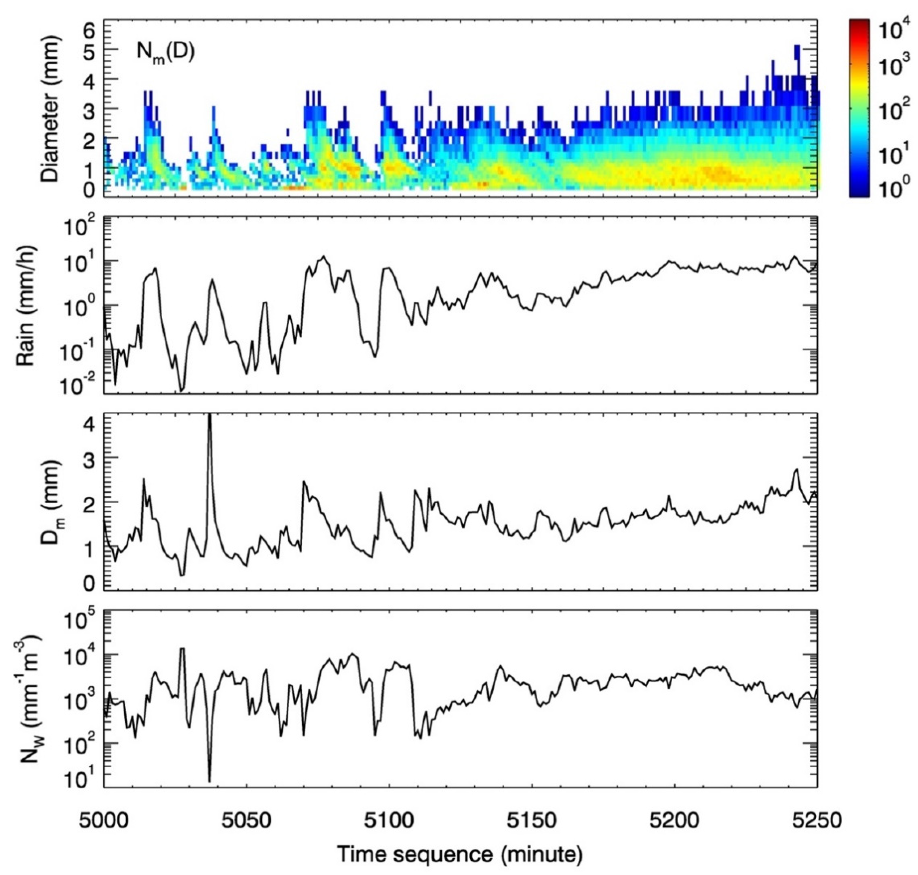
As an example,
Figure 1 shows a segment of DSD data versus time taken from one of the PARSIVEL disdrometers over 250 min. The image of N
m(D) is given in the top panel with respect to D along the ordinate and time (minute) along the abscissa. R and D
m computed from N
m(D) are given in the 2nd and 3rd panels, respectively, for the same time period. In addition, the normalized intercept parameter, N
w in mm
−1m
−3, of the DSD, when the DSD is parameterized as a gamma distribution, is also provided in the bottom panel. The definition of N
w will be detailed in
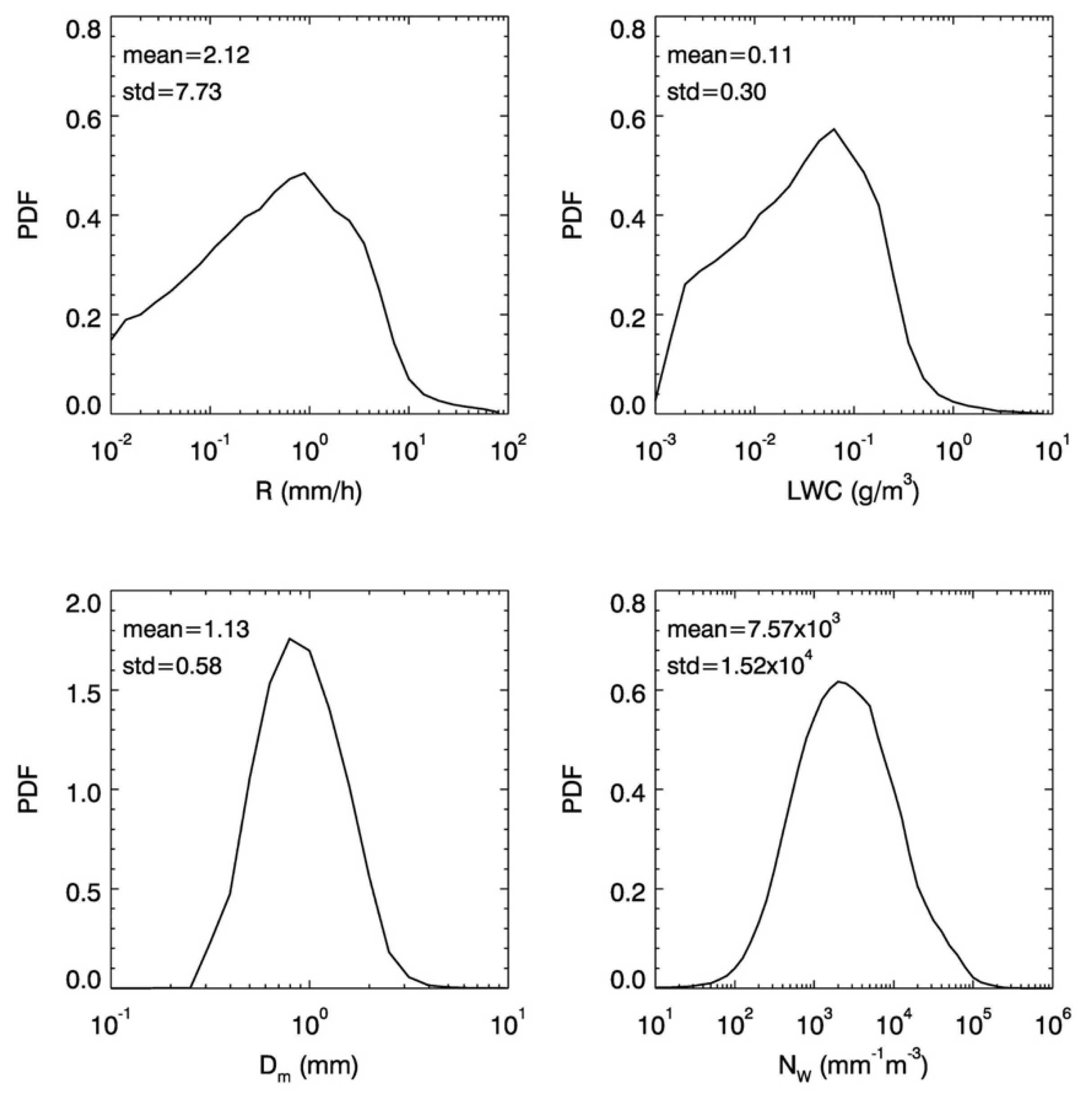
Section 3. To illustrate frequency of occurrence in the data,
Figure 2 provides the probability density functions (PDF) of R (top-left), liquid water content (LWC in g/cm
3) (top-right), D
m (bottom-left) and N
w (bottom-right) from the entire datasets collected from the disdrometers that have 213,465 one-minute DSD spectra in total. As clearly shown in
Figure 2, the PDFs of logarithms of D
m and N
w closely follow the Gaussian distributions with their means of 1.13 mm and 7.57 × 10
3 mm
−1m
−3, respectively, while the PDFs of logarithms of R and LWC appear asymmetrical to their respective means of 2.12 mm/h and 0.11 g/m
3. Additionally, the standard deviations of R, LWC, D
m and N
w are 7.73 mm/h, 0.30 g/m
3, 0.58 mm and 1.52 × 10
4 mm
−1m
−3, respectively.
3. The Gamma DSD Model
The gamma distribution has been widely used to represent rain-drop size distribution N(D) (mm
−1m
−3) as a function of raindrop diameter D (mm). Its general form is given by:
where N
0 is the intercept parameter, µ is the shape factor, and Λ is the slope parameter expressed as:
D
m is the mass-weighted mean diameter given by:
where M
3 and M
4 are the 3rd and 4th moments of N(D), respectively. The ith moment of DSD is defined by:
Substituting N(D) of Equation (6) with Equation (3) and using the gamma function, we obtain:
The liquid water content (LWC) in g/m
3 is:
Note that water mass density with its value of 1 g/cm
3 is suppressed in Equation (8). From Equation (8), N
0 is:
Inserting N
0 of Equation (9) into Equation (3) and then re-organizing it using Equation (4), we arrive at:
N
w is in units of mm
−1m
−3, and often called as the DSD normalized intercept parameter while f(µ) is unitless. The form of the gamma distribution expressed in Equation (13) is widely used in rain and snow precipitation retrieval [
7,
9,
16,
17,
18,
19,
24]. From Equation (13), the rainfall rate is given by:
where V(D) is raindrop fall velocity (m/s) and is expressed as a function of the raindrop diameter proposed by Lhermitte [
25]:
It is important to note that R, LWC, D
m and N
w are the bulk parameters that can be derived directly from DSD data without assuming a DSD model. Equation (11) yields an analytical relationship among the quantities LWC, D
m and N
w, from which it follows that from any two DSD bulk parameters LWC, D
m and N
w, the third is determined uniquely. To explore the possibility of a similar relationship among R, D
m and N
w, two approaches are investigated. One is based on the DSD-based regression from which a power-law fit is performed between the R/N
w and D
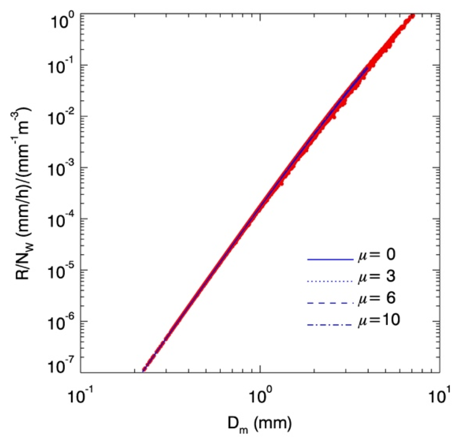
m data that are derived directly from the measured DSD. The second approach is to compute the same quantities from the DSD gamma model. Shown in
Figure 3 are the DSD-based and model-based results, i.e., the ratios of R to N
w as a function of D
m. The model results are given by various line-style blue curves computed at µ values of 0, 3, 6 and 10 while the red filled-circles are those derived from the measured DSD (213,465 1-min DSD spectra). It is not difficult to find that the model results are nearly independent of µ as demonstrated by the fact that the curves are indistinguishable for different µ values. These results, however, almost perfectly coincide with those from the DSD measurements that show little variation in log-log space. The power-law regression is applied to the gamma DSD model data for µ values assumed from 0 to 10. This gives:
where
From above equation, we have
To check the validity and accuracy of Equations (16)–(18), used to reproduce R, D
m and N
w, we employ the aforementioned DSD data and compare the estimates of R, D
m and N
w to the same quantities derived directly from the DSD data. For example, R, as estimated from (16) with inputs of the DSD-derived D
m and N
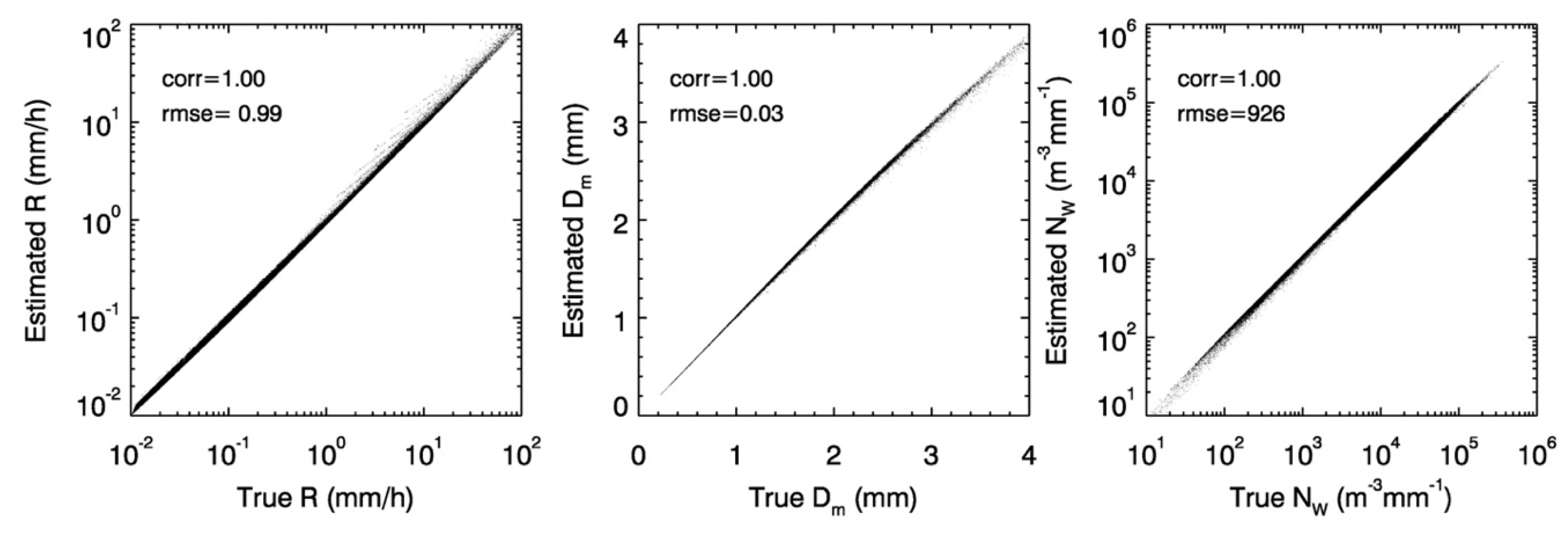
w, is compared against the value obtained directly from the corresponding measured DSD spectrum. For simplicity, the quantities obtained from the DSD data are referred to as truth or true values while those that are derived from Equations (16)–(18) are referred to as the estimates. Provided in
Figure 4 are the scatter plots of the estimates of R (left), D
m (middle) and N
w (right) versus their respective true values. Not surprisingly, the comparisons made in
Figure 4 reveal excellent agreement between the estimates and truth, evidenced by the fact that there are nearly perfect correlations (that round to 1.00) and small rms (root mean square) errors (0.99 mm/h in R and 0.03 mm in D
m) despite the rms error in N
w (926 mm
−1m
−3), which, however, is still fractionally small in view of its large dynamic range and mean value of 7.6 × 10
3 mm
−1m
−3. It is worth reiterating that the Equations (16)–(18) are based on the gamma DSD model with μ ranging from 0 to 10 rather than the measured DSD data, and are therefore independent of the measured DSD data that vary seasonally as well as geographically. Agreement between the estimates and their true values indicate that D
m and N
w can be used to characterize R with sufficient accuracy.
4. Rainfall Rate–Mass-Weighted Diameter (R–Dm), Normalized Intercept Parameter (Nw)–R and Nw–Dm Relations
Figure 3 suggests that three variables of R, D
m and N
w are closely related, and their relations are given by Equations (16–18). However, in many situations of rain retrieval, the radar equations are often under constrained, which means that there are more unknown variables than the number of equations as a result of limited independent radar measurements. As such, the constraints among the DSD parameters as in Equations (16–18) need to be relaxed to some extent to make the retrieval solutions robust and achievable. One important example of this situation is the GPM DPR operational algorithm that takes on a nominal R–D
m relation along the radar profile and then applies an adjustable parameter ε to modify the R–D
m relation to minimize the cost function [
9,
26]. This cost function depends on several factors, one of which is minimizing the difference of independently measured path attenuations between Ku- and Ka-band. Other factors are the mean and standard deviation of the Gaussian distribution of ε as well as the rms difference between the simulated and measured Ka-band reflectivities. To exploit the R–D
m, N
w–R and N
w–D
m relationships and also explore their correlations, the DSD data are employed.
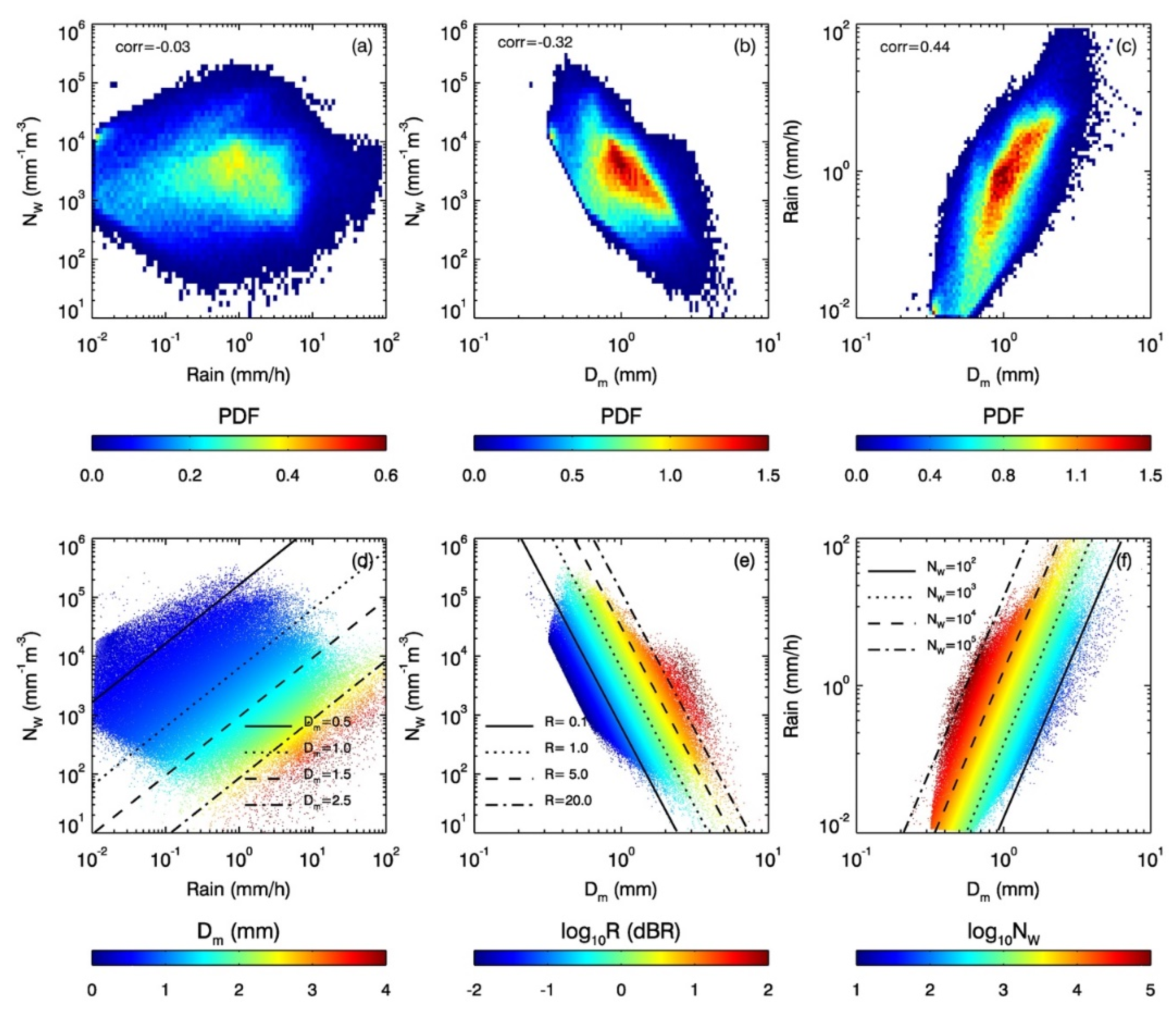
Figure 5 illustrates the two-dimensional PDFs of N
w–R (
Figure 5a), N
w–D
m (
Figure 5b) and R–D
m (
Figure 5c) as well as their corresponding scatter plots of N
w–R (
Figure 5d), N
w–D
m (
Figure 5e) and R–D
m (
Figure 5f). The pixel colors of the bottom panel show the mean values of D
m (
Figure 5d), logarithms of R (
Figure 5e) and N
w (
Figure 5f) in the planes of N
w–R, N
w–D
m and R–D
m, respectively. The theoretical model computations from the gamma DSD with a fixed µ of 3 are also superimposed on the plots. As shown in
Figure 5, the correlation between N
w and R is −0.03, indicating that they are nearly uncorrelated. The correlations of N
w–D
m and R–D
m are −0.32 and 0.44, respectively. These results indicate that a large amount of uncertainty would occur in estimating R from N
w alone, but this uncertainty will be reduced if D
m is used instead. Also, there exists a certain degree of error in inferring N
w from D
m without knowing R. The colored scatter plots of
Figure 5 in fact reveal how the two-parameter relations are a function of the third one. In the logarithmic scale of N
w and R the data points with constant D
m lie along ~45° straight lines and move toward the bottom-right direction as D
m increases. Likewise, the contours of R in N
w–D
m and N
w in R–D
m are straight lines and parallel to one another which are plotted in logarithmic scales. The image pattern that changes slowly with D
m and spans vast area along the direction perpendicular to constant D
m lines, as shown in the N
w–R plane (
Figure 5d), reveals large variation in the N
w–R relation, indicating a strong dependence of the N
m–R relation on D
m. On the other hand, the relatively small variations shown in the images of N
w–D
m (
Figure 5e) and R–D
m (
Figure 5f) imply relatively weak dependencies of N
w–D
m on R and R–D
m on N
w.
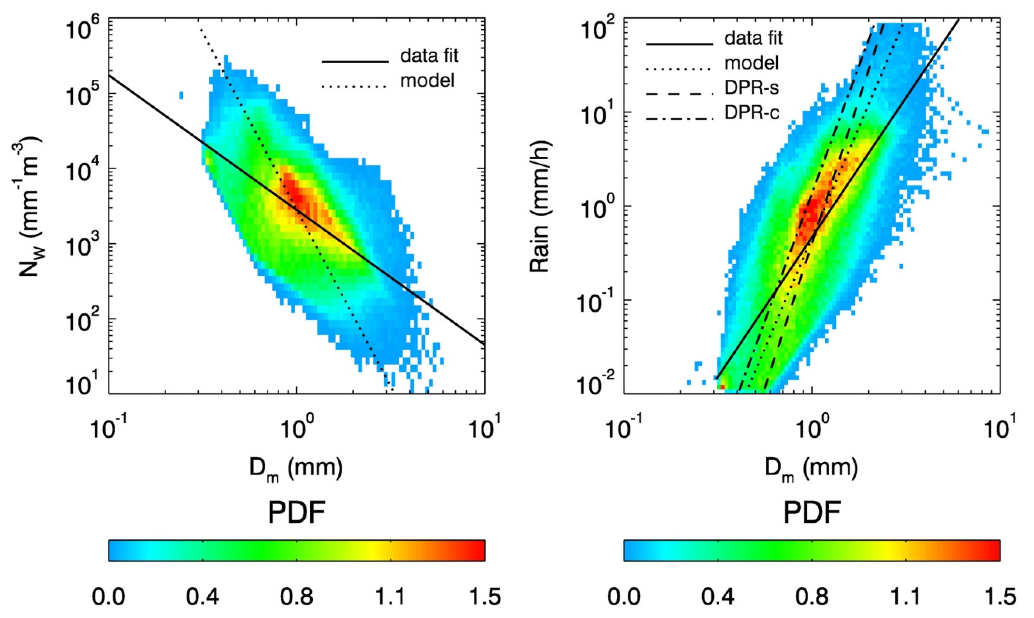
Figure 6 displays the power-law fittings of N
w–D
m (left) and R–D
m (right) to the data along with the DSD model results. The solid lines are the results that are statistically fitted to the data by using the method of least-squares, and the dotted lines are those with the exponents fixed at the values found in Equations (16) and (18), i.e., −4.706 for the N
w–D
m relation and 4.706 for the R–D
m relation, with which the scale factors are fitted to the data. The fitting curves using the DSD model-derived exponents are denoted by ‘model’ in the plots. For comparison, the DPR-default R–D
m relations are also provided, in which the notations of ‘DPR-s’ and ‘DPR-c’ represent the cases of stratiform and convective rain, respectively. The resultant fitting coefficients are summarized in
Table 1. Because of large variations in the data between N
w and D
m as well as R and D
m, as reflected by their moderate correlations shown in
Figure 5, the regressions to these data depend on the methods selected and physical models applied. The model-based regressions, though they differ from the data fittings, represent fairly well the N
w–D
m and R–D
m relations judging by their consistency with the PDFs. It is worth reiterating that R and N
w are constant along the model-based N
w–D
m and R–D
m fitting curves, respectively. The R–D
m relation based on the DSD model agrees better with the nominal R–D
m relations adopted by the DPR standard algorithm than the relation that is obtained by fitting directly to the data.
5. DSD Bulk Parameters Linked to Ku- and Ka-band Radar Parameters
As discussed above, the DSD bulk parameters R, D
m and N
w are closely interrelated. These parameters are of importance for precipitation modelling and weather prediction studies. The relation between radar parameters and these DSD bulk parameters comprises a basis for radar rain retrieval. Although the purpose of our study is to explore applications to the Ku- and Ka-band dual-frequency radar, development of the full radar algorithm for the retrieval of rain profiles is beyond the goal of this paper. To establish the statistical characteristics of relationships between the DSD and dual-frequency radar parameters, such as Ku- and Ka-band radar reflectivity factors, the radar reflectivities are simulated by prescribing raindrops as oblate spheroids whose axis ratios yield the shape–size relations described by Thurai et al. [
27]. The T-matrix method [
28] is applied to obtain the scattering properties of single particles assuming a nadir-viewing radar and taking the major axes of raindrops to be in the horizontal plane. It should be noted that the raindrop diameter throughout the paper actually refers to an oblate drop with a volume-equivalent diameter D. Because of the fact that the Ku- and Ka-band radar signals are attenuated by raindrops while propagating through rain, attenuation corrections to the measured reflectivities are needed before the DSD retrieval. Specific attenuations (dB/km), denoted by k
Ku and k
Ka at Ku- and Ka-band, respectively, are the parameters that are used to account for the attenuation along the propagation path to the range gate at which the retrieval occurs. In addition to R, D
m and N
w, the estimates of k
Ku and k
Ka are crucial for development of radar profiling algorithms. Conventionally, the specific attenuation is fitted to measured DSD in terms of reflectivity factor, such as k
Ku–Z
Ku and k
Ka–Z
Ka relations. These relations have been widely used for single-frequency radar retrieval [
5,
29,
30]. However, k
Ku and k
Ka could be better estimated if both the Ku- and Ka-band reflectivities were used. In dual-frequency radar applications, one of the most important parameters is the dual-frequency ratio (DFR), which is defined as
where Z
Ku and Z
Ka are the radar reflectivity factors at the Ku- and Ka-band, expressed by
where λ is wavelength, referring to either Ku- or Ka-band, and σ
b(D,λ) is the backscattering cross section of a particle with diameter of D. By convention, |K
w|
2 is taken to be 0.93 for liquid water. DFR has many applications ranging from snow and rain retrievals to hydrometeor phase identification [
2,
24,
31,
32].
For the gamma DSD model given in Equation (13), DFR is independent of the N
w, and therefore D
m is directly related to DFR for a given μ. Other parameters like R, N
w, k
Ku and k
Ka, however, are a function of not only DFR but also Z
Ku or Z
Ka. To link these parameters to the DFR and Z
Ku, the R, N
w, k
Ku and k
Ka are first normalized by Z
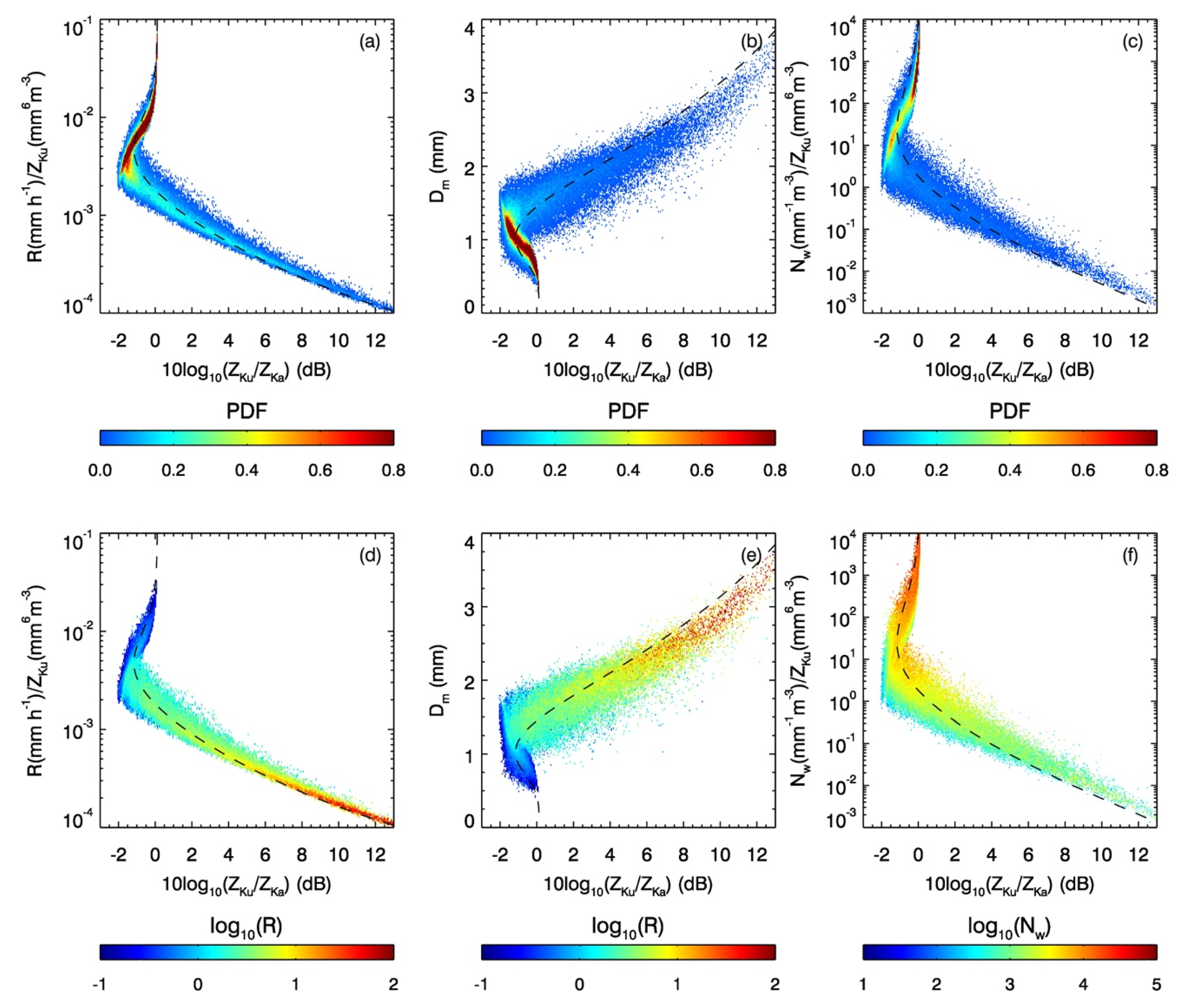
Ku, and then these normalized parameters are related to DFR. The top panel of
Figure 7 provides the PDFs of the data obtained from the measured DSD in the planes of R/Z
Ku–DFR (
Figure 7a), D
m–DFR (
Figure 7b) and N
w/Z
Ku–DFR (
Figure 7c). Similar plots are made in the bottom panel of
Figure 7. Instead of the PDFs, the bin-averaged R on logarithmic scale in the R/Z
Ku–DFR (
Figure 7d) and D
m–DFR (
Figure 7e) planes as well as logarithmic N
w in the N
w/Z
Ku–DFR (
Figure 7f) plane are plotted. The PDFs reveal two-dimensional distributions of occurrence frequencies of the data in the planes comprising DSD and radar parameters while the images of the lower panel reflect changes in R and N
w. For example, in the PDF of R/Z
Ku vs. DFR (
Figure 7a) most of the DSD data are clustered in the region where DFR values are small, and the rain rates of these data increase with DFR as shown in the bottom-left image. The plots show that there exist two values of the normalized DSD parameters for a given DFR in the regions where DFR is less than 0, which typically correspond to light-to-moderate rain with averaged D
m less than 1 mm and N
w greater than 10
3 mm
−1m
−3. Beyond these regions, however, good correspondences are found between the DSD parameters of R, D
m and N
w and the radar parameters of Z
Ku and DFR. This actually offers a means to infer the DSD parameters from the radar measurements. In particular, R can be estimated by, first, deriving R/Z
Ku from DFR and then multiplying the result by Z
Ku. The same procedure can be applied to estimate N
w. D
m, on the other hand, is directly obtained from DFR. For reference, the computational results from the gamma DSD model with a fixed μ of 3 (black dashed lines) are also plotted in
Figure 7. The gamma model appears to be a reasonably good approximation (dashed lines) from the perspective of the Ku- and Ka-band retrieval.
The issue of double solutions when DFR < 0 inevitably leads to large ambiguities in the DSD retrieval. The small, negative values of DFR are a consequence of the fact that the Ku- and Ka-band reflectivities are nearly identical for the case of light rain which is composed primarily of small raindrops. In these cases, Rayleigh scattering, where the backscattering cross section is proportional to the 6th power of particle diameter and independent of radar frequency, dominates at both frequencies. If the Ku- and Ka-band radar falls into the Rayleigh scattering regime, the 2nd frequency measurement basically doesn’t provide additional information. It is worth noting that out of 213,465 1-min DSD spectra employed in this study, nearly half of them are either in the double-solution region or under the Rayleigh scattering. An attempt to mitigate the double-solution impact has recently been studied by Liao and Meneghini [
12].
Comparison of the gamma DSD results with those computed directly from the DSD data suggests that there is less uncertainty in the estimates of R than in the estimates of D
m and N
w for the region where DFR > 0 because of the fact that relatively small variability is found in R given a pair of DFR and Z
Ku values as compared with D
m and N
w. As mentioned earlier, the DSD model results shown in
Figure 7 are from the gamma DSD with μ = 3, which is the case for the GPM DPR operational algorithm [
33]. The results from the gamma DSD with different μ are also computed (not shown), and reveal that there are only small changes in the estimates of R. This, however, is not the case for either D
m or N
w.
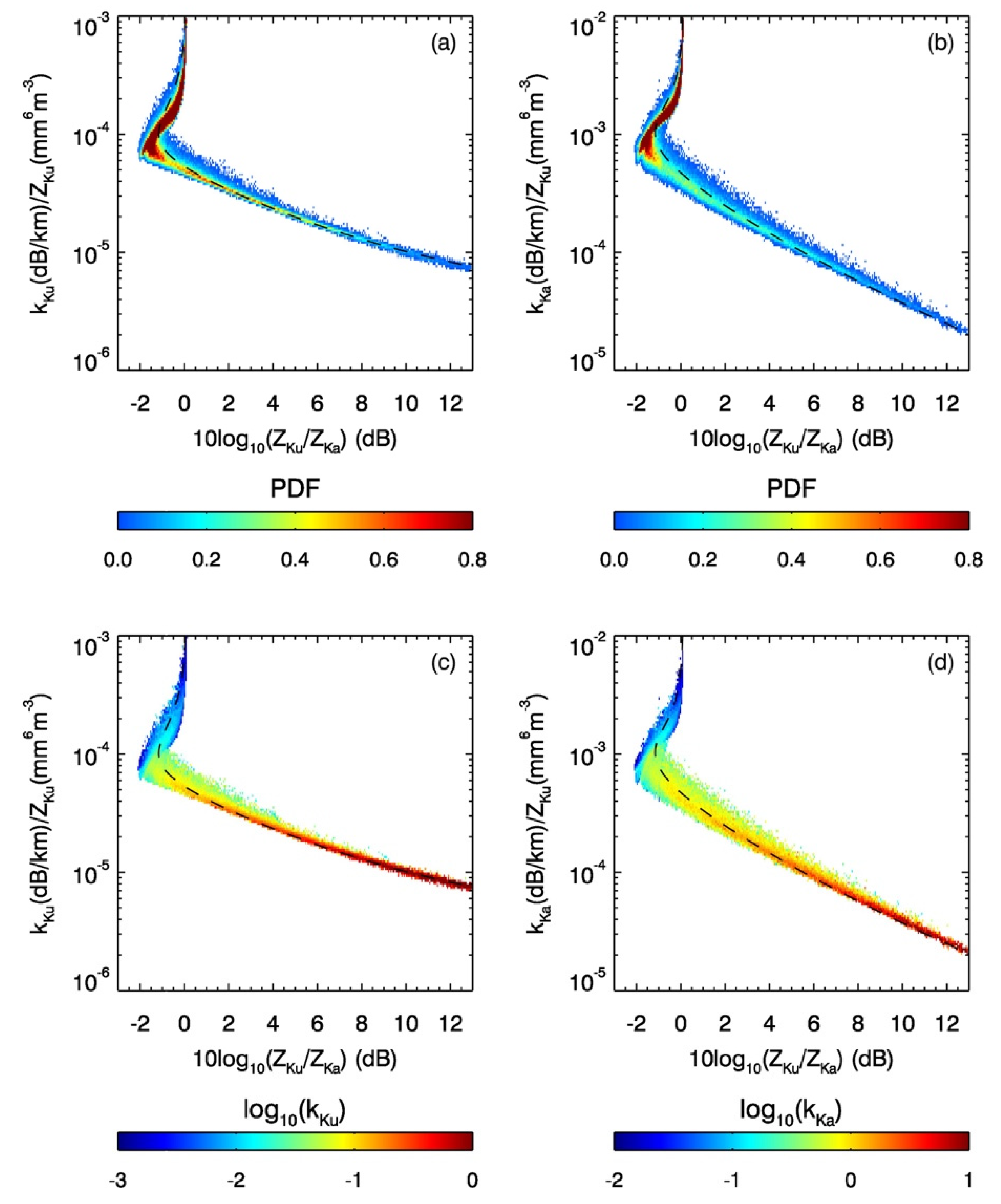
Similar to
Figure 7,
Figure 8 displays the PDFs (
Figure 8a,b) of the Z
Ku-normalized specific attenuations versus DFR and the bin-averaged specific attenuations (
Figure 8c,d) at Ku- (
Figure 8a,d) and Ka-band (
Figure 8b,d). The results shown in
Figure 8 resemble many of the features found in
Figure 6, i.e., there are the double-solution regions that are identical to those found in R, D
m and N
w. In the region when DFR > 0, k
Ku and k
Ka increase with an increase of DFR, and show relatively small spreads as seen in the PDF plots. Again, the fixed μ = 3 gamma DSD results denoted by black dashed curves, show good approximations to those obtained from the DSD data. While the combination of Z
Ku and DFR leads to fairly good estimates of k
Ku and k
Ka, as in the estimates of R, D
m and N
w, the application to the double-value region still remains a challenge.
6. Summary and Conclusions
With the use of 213,465 one-minute-integration-time DSD measurements collected during the field campaigns at three geographically different sites and also with use of the gamma DSD model, the statistical interrelationships among the DSD bulk parameters of R, Dm and Nw are studied. According to the definition of Nw, there exists an analytical relationship between LWC, Dm and Nw. To explore similar relationships among the variables R, Dm and Nw, a power-law fit is applied to the data of R/Nw and Dm computed from the gamma DSD model with various μ values. It is found that the model-simulated R/Nw vs. Dm results are nearly independent of µ. Furthermore, they conform well with those derived from the DSD data. Like the model results, the measured DSD show very little spread, implying a very strong relationship between R, Dm and Nw. This leads to the conclusion that R can be determined with high accuracy if Dm and Nw are known. A similar conclusion holds for Dm and Nw, i.e., Dm can be derived from R and Nw, and Nw can be obtained from R and Dm with a high degree of accuracy Comparisons among the estimates of R, Dm and Nw from the fitting equations to their respective true values demonstrate that nearly perfect correlations exist between the estimates and the true values with negligibly small rms errors.
Although R, D
m and N
w are closely interrelated and one parameter is accurately expressed as a function of the other two parameters as in Equations (16)–(18), i.e., three-parameter relations, the constraints among these variables sometimes need to be loosened to be consistent with the limited number of radar measurements. In many situations where the radar equations are under constrained, the three-parameter relations of R, D
m and N
w need to be replaced by two-parameter relations. It is then useful to investigate statistical relationships between R and D
m, N
w and R, and N
w and D
m as in previous studies [
18,
26,
34]. It is found from this study that R and D
m are moderately correlated while N
w and D
m are moderately negatively correlated. N
w and R, however, are uncorrelated. Because of the generally weak correlations in these two-parameter relationships (R–D
m, N
w–R and N
w–D
m), the data spread is relatively large, resulting in large errors in the estimates. Large variability in the two-parameter relationships is caused by not taking into account variations in the third parameter. For example, variability of the R–D
m relation is the result of variation in N
w. To improve retrieval accuracy by lessening the uncertainties of the two-parameter relations, additional constraints are sometimes adopted, such as the GPM DPR that is based on adjustable R–D
m relation with which an adjustable parameter ε is fixed throughout the range gates of one profile but varies from profile to profile. It is worthwhile mentioning that adjusting ε in the R–D
m relation would be equivalent to an adjustment of N
w if the exponent of the R–D
m relation is set to the value of 4.706 as derived from the fixed-μ gamma DSD. However, the exponents of the R–D
m relation implemented in the GPM DPR algorithm are 6.131 and 5.420 for stratiform and convective rain, respectively, leading to change of N
w with D
m in a way by which N
w is proportional to
and
for stratiform and convective storms, respectively. Use of adjustable R–D
m relation for the DSD profiling retrieval originates from the concept of the ‘two-scale’ DSD model proposed by Kozu and Nakamura [
35] that allows one DSD parameter being constant over a certain space or time domains while another DSD parameter changes dynamically. Employing two-year DSD data in testing rain retrieval, they found that constant drop number concentration N
T (the 0th moment of DSD) or constant N
0 of (9) seems to be reasonable. Based on our analysis of the gamma DSD-based regression among R, D
m and N
w, constant N
w of the ‘two-scale’ model is perhaps another practical choice. Further study is required to examine the sensitivity of the DSD estimates to the choice of constant DSD parameters or different exponents of the R–D
m relation toward understanding and improvement of the GPM DPR performance in estimates of DSD parameters.
Our study has also been extended to look into the statistical characterization of relationships between the DSD parameters on one hand and the Ku- and Ka-band dual-frequency radar parameters on the other. To account for rain attenuation, specific attenuations are included. D
m is directly related to DFR. In contrast, R and N
w, as well as k
Ku and k
Ka, depend not only on DFR but also on Z
Ku or Z
Ka. To relate them to the dual-frequency radar measurements, a Z
Ku-normalization factor is used so that the Z
Ku-normalized R, N
w, k
Ku and k
Ka, which are obtained from the measured DSD, can be expressed as a function of DFR. The theoretical computations from a fixed μ = 3 gamma DSD model are compared with the DSD-simulated results. Comparisons of the results shows fairly good agreement between the model computations and DSD data. Not surprisingly, there exist double-solution regions where DFR < 0, in which two values of the estimates are detected for a given DFR. Since no independent information is available to aid in selection of the solution, the double solutions lead to ambiguities in the estimates. A few methods attempting to mitigate the double-value issues include use of the modified dual-frequency standard technique [
12] and use of the R–D
m relation [
9,
26]. In the region with DFR > 0, a robust one-to-one relation between DFR and normalized DSD and specific attenuation parameters ensures the soundness of the retrieval. Analysis of the results also indicates that there are smaller uncertainties in the estimates of R than in the estimates of D
m and N
w as a result of the relatively small variability in R as compared with that in D
m and N
w. In addition, the combination of Z
Ku and DFR leads to fairly good estimates of k
Ku and k
Ka if the DFR is positive.


