The Polar Vortex and Extreme Weather: The Beast from the East in Winter 2018

Abstract

Public attention has recently focused on high-impact extreme weather events in midlatitudes that originate in the sub-Arctic. We investigate movements of the stratospheric polar vortex (SPV) and related changes in lower atmospheric circulation during the February-March 2018 “Beast from the East” cold winter event that dramatically affected much of Europe and north-central North America. This study demonstrates that the movement of the SPV is a key linkage in late winter subarctic and northern midlatitude extreme weather events. February–March 2018 saw two types of subarctic-midlatitude weather connections. In the first type, the SPV was displaced from the pole to lower latitudes over North America in February and then was found over northern Siberia in March. Mid-February and mid-March are examples of persistent near vertically aligned geopotential height structures of the atmospheric circulation. These structures over North America and Eurasia advected cold Arctic air southward. The second type of cold surface event was associated with a weak regional SPV and a sudden stratospheric warming event over Europe during the second half of February. These late winter linkage events that arise through dynamic instabilities of the SPV are more common in the last decade, but the potential role of enhanced Arctic amplification is uncertain.

1. Introduction

In the Northern Hemisphere winter, a stratospheric polar vortex (SPV) develops over the North Pole, with strong zonal westerlies circulating around low temperatures at the center of the vortex [1]. Impacts of SPV events are not confined to the stratosphere. Dynamical coupling with the troposphere can cause an eddy-driven jet stream shift southward and result in extreme weather over parts of Eurasia and North America [2]. Although the SPV is typically thought of as being centered on the Arctic, in reality its center is often found in the subarctic, over northern Canada or northern Eurasia. During January–February 1979–2018, SPVs at 100 hPa were found approximately 40% of the time over the North American side and 25% over the Siberian side [3]. Although continental cold air outbreaks can occur without a SPV connection, a southward-shifted SPV is often associated with severe surface weather, cold temperatures anomalies, snow and record storms and rainfall that arise from the tropospheric polar jet moving equatorward and a weakening jet stream [2,3,4,5,6]. Such examples were found in February and March 2018. A SPV located over North America in February contributed to extreme low temperatures to the northern plains, and allowed high surface pressure with low temperatures to develop over Central Europe that moved westward over the United Kingdom and as far south as Italy [7]. In March, the center of the SPV relocated over Eurasia and was associated with cold air advection over Europe. Both European events have been referred to as “the Beast from the East” but they were associated with different synoptic situations, as we demonstrate.

As the SPV has a major role as a linkage in late winter subarctic and northern midlatitude extreme weather events [5,8,9], a closer examination of February–March, 2018, as a case study is in order.

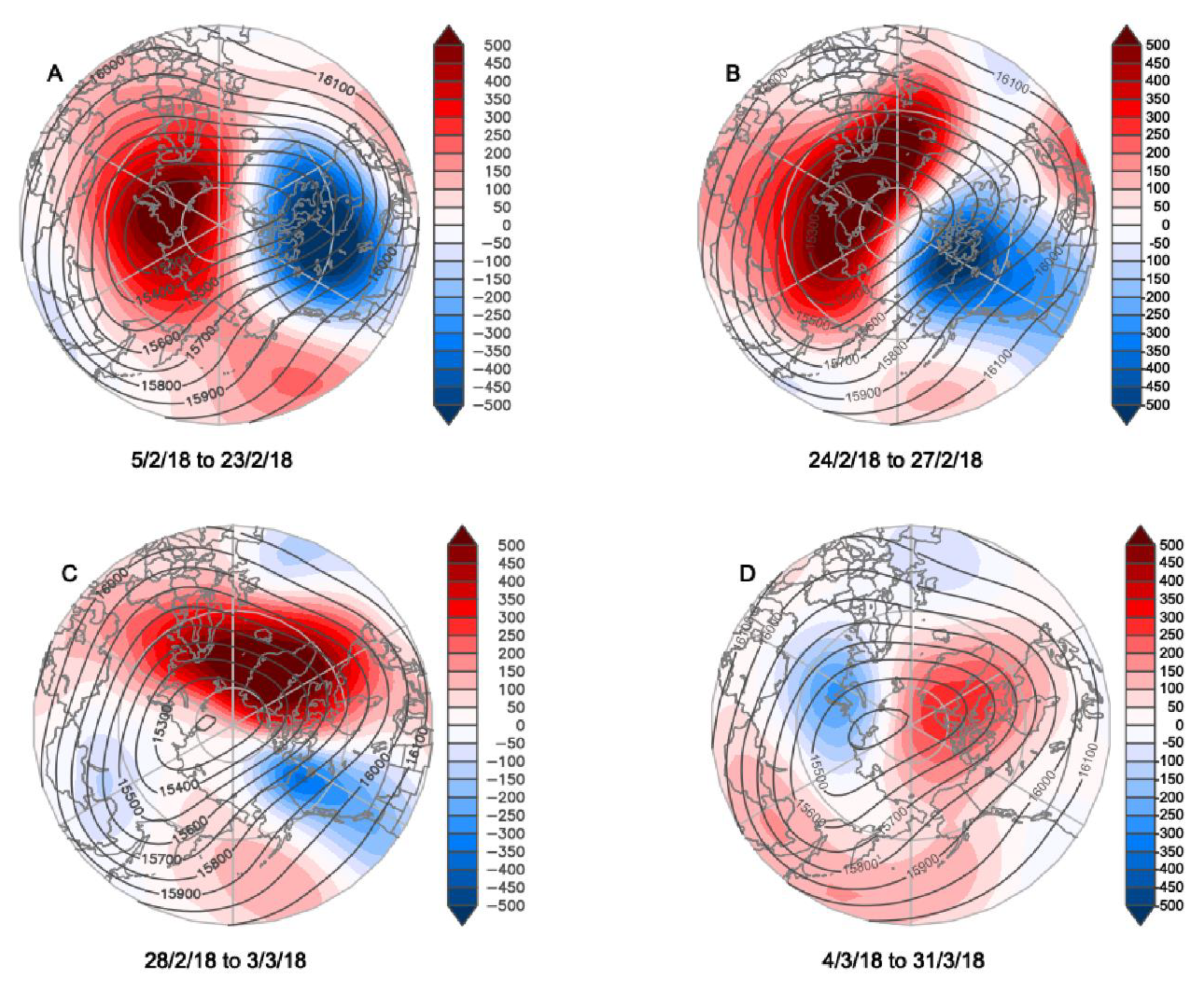
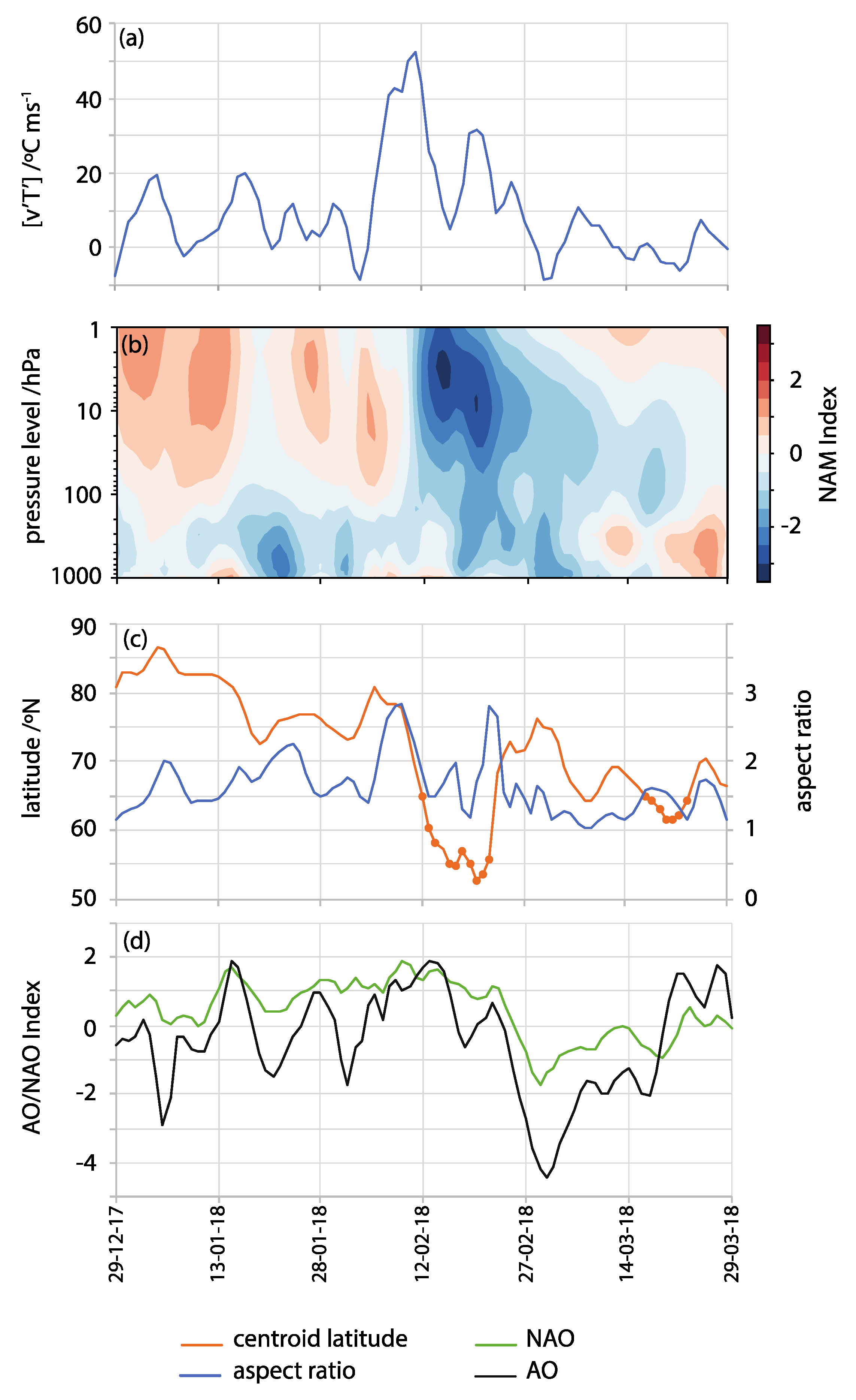
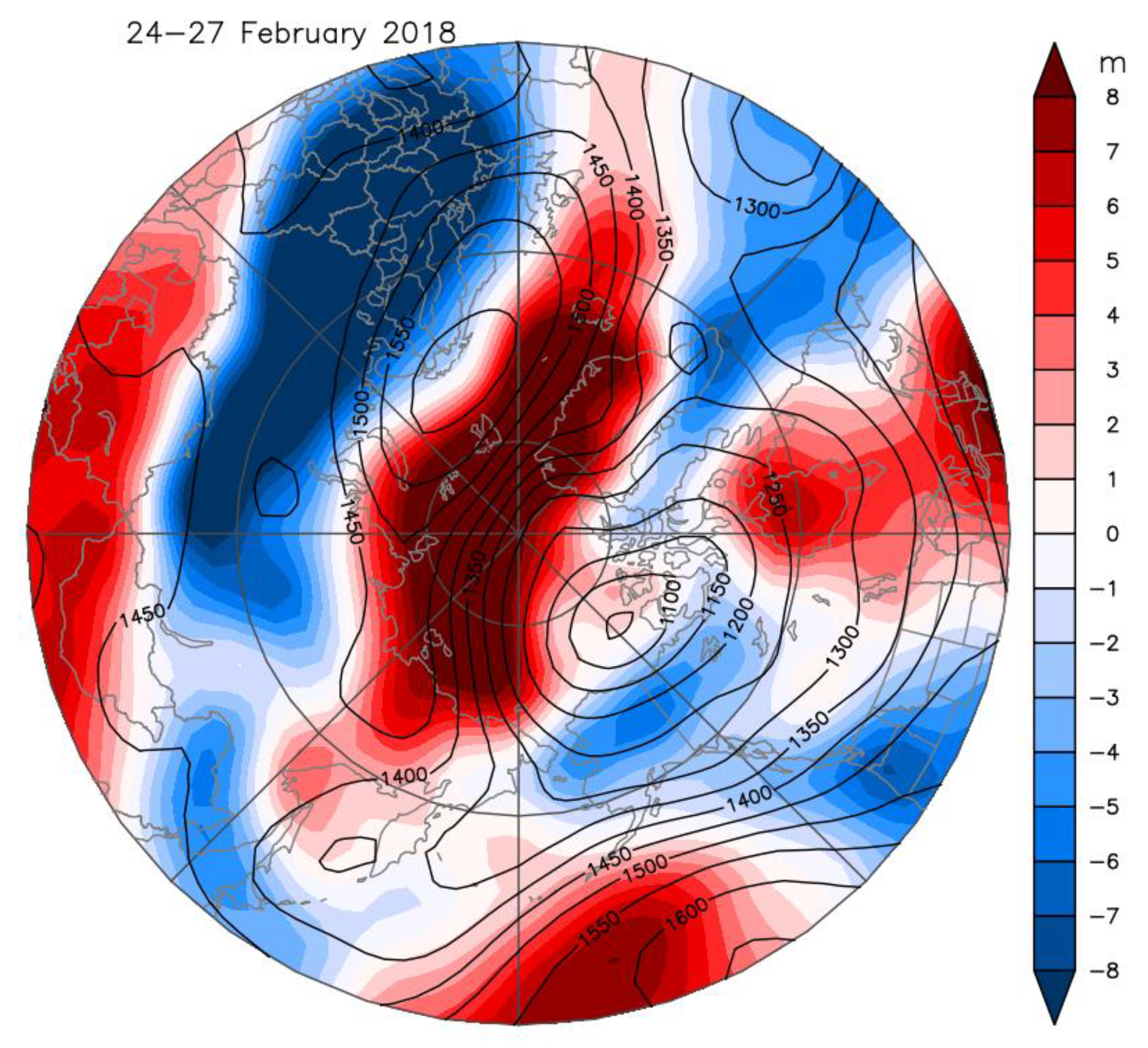
2. Stratospheric Polar Vortex: February–March, 2018

Based on the National Centers for Environmental Prediction-National Center for Atmospheric Research (NCEP–NCAR) reanalysis [10], Figure 1 tracks the geopotential height field at 100 hPa for February–March 2018; each sub-figure captures a period of relative stationarity. SPV anomalies in the lower stratosphere are known to have strongest coupling to the surface weather (e.g., [11]); hence we use a 100 hPa geopotential height field to illustrate the evolution of the vortex. A weakening of the SPV occurred through most of February and March, with a sudden stratospheric warming (SSW) [12,13,14,15] onset in mid-February. The SPV, after being centered near the North Pole for January, 2018 (not shown), was split with a stronger center persistent over northeastern Canada for most of February (Figure 1A), and a secondary center over Siberia. This North American vortex then migrated westward. A SPV was located over the northern coast of Siberia for much of March (Figure 1D).

The persistence and local intensification of the displaced SPV, and their downward impacts on midlatitude waves can be dynamically supported by temporal evolution of the potential vorticity (PV). In February (Figure 2A), two positive PV anomaly centers were located over northeastern North America–East Greenland Sea and Eastern Eurasia, corresponding to the split of the SPV to two local centers over these two regions as shown in Figure 1A. The positive PV anomaly over North America shows a stronger intensity. A positive/negative PV anomaly is defined as the local maximum/minimum PV value. According to the PV dynamics theory (e.g., [16]), it dynamically intensified and supported the increased persistence of the tropospheric low-pressure system. Displaced SPVs can show stronger negative surface pressure anomalies collocated with changes in tropopause height which are indicative of a response to PV anomalies in the lower stratosphere [13]. Additionally, there was enhanced poleward heat transport in the North Atlantic sector.

The weak SPV on the Eurasian side of the Arctic during late February was associated with a SSW [12,13,14,15]. Coupling can take place between the SPV and the tropospheric circulation that can result in extreme weather at the surface at lags of up to 40 days [11,17,18]. Using a definition of SSWs based on vortex moments of the 10 hPa geopotential height field, a split SSW event is identified when the aspect ratio (elongation of the vortex) exceeds 2.4 for seven or more days, while a displacement event is when the centroid latitude lies south of 66° N for at least seven days [13]. An advantage of this method is that it is based on vortex geometry rather than zonal mean values.

Figure 3 shows features of the SPV, SSW, and atmospheric circulation indices at lower levels for winter 2017–2018. The large increase in the meridional eddy heat flux at 100 hPa from early to mid-February represents the upward influence of the troposphere (Figure 3A), indicating an upward propagation of planetary waves that reinforced the late February SSW event. The Northern Annular Mode (NAM) Index, calculated as the inverse of the polar cap geopotential height anomaly averaged over 65–90° N at different atmospheric levels, demonstrates the downward propagation of the negative NAM anomalies (Figure 3B) following the pronounced increase in upward wave activity flux shown in Figure 3A. This suggests an SSW contribution to the tropospheric anomalies during the second half of February [14,19]. We use NAM for calculating at all atmospheric levels while the Arctic Oscillation (AO) is reserved for the 1000 hPa level. While there is a brief period of vortex splitting prior to 12 February according to the moments method, this SSW is identified primarily as a displacement event. There is a 10-day period when the vortex is displaced southward of 66° N (Figure 3C), starting before 12 February-the date of the SSW onset. This date is also identified as SSW onset by a wind reversal diagnosis [12,20]. As the vortex moves poleward again, there is a second brief elongation of the vortex (increased aspect ratio). Following, as the vortex starts to move equatorward, there is a lagged response in the AO and North Atlantic Oscillation (NAO) surface indices (Figure 3D), and these indices continue to become more negative after the vortex displacement has recovered, reaching minima around 18 days after the onset of the SSW in the stratosphere.

The transition of the primary center of the SPV from North America (Figure 1A) via central Arctic to Siberia (Figure 1B,C) took 10 days (from 22 February to 4 March) and was related to the strengthening of a ridge in the geopotential height field over the Atlantic (Figure 1B,C). The feature has the characteristics of a warm-anticyclonic wave-breaking atmospheric blocking pattern [23,24], and was reflected in a dramatic increase in daily values of the Greenland Blocking Index (GBI) [25] from −1.14 on 23 February to record high values in the NCEP/NCAR reanalysis-based series dating back to 1948 on 1–3 March, peaking at +3.03 on 2 March 2018. The daily NAO on 1 March was the second lowest in the time series since 1948.

The North American positive PV anomaly contributed to the late February SPV transition due to a negative PV anomaly intrusion into the Icelandic and Norwegian Seas. The time evolution of the PV anomalies during this process demonstrated wave breaking, causing a blocking ridging pattern and an increase of surface high pressure over northern North Atlantic and Scandinavia. This dynamic process favored the development of a negative NAO (e.g., [26]). According to [27], wave breaking is intensified following periods of weak SPV, which implies that this wave breaking episode is consistent with a downward SPV influence on the tropospheric dynamics.

The breakdown of the long-wave pattern relates to the strong northward wind component in the western North Atlantic (Figure 1B) and the final predominance of the westward propagation of the Rossby wave (Figure 1C) [28]. References [29] and [14] note that SPV location translations often are associated with blocking events.

In March, the strongest positive PV anomaly shifted to the Eurasian side of the Arctic centered over the Barents and Kara Seas (Figure 2B) that persisted for most of March. Correspondingly, the SPV center was located in the same location as the negative anomalies show in Figure 1D, above the low geopotential height center at 850 hPa. The low geopotential heights from the troposphere to the lower stratosphere shows a near vertical alignment. The intensification and persistence of this structure can be attributed to the strong positive PV anomaly. A recent study examined persistence mechanisms of an intense and long-lived Arctic cyclone system [30]; it showed that downward intrusion of the positive PV anomaly generates a cyclonic jet around the tropopause and, in turn, maintains the tropospheric cyclonic circulation. At the same time, the temporal variation of the PV anomaly extension southward resembled anticyclonic wave breaking. Both stationary low pressure over the Barents–Kara Seas and wave breaking favor the establishment of high pressure over Eurasian midlatitudes.

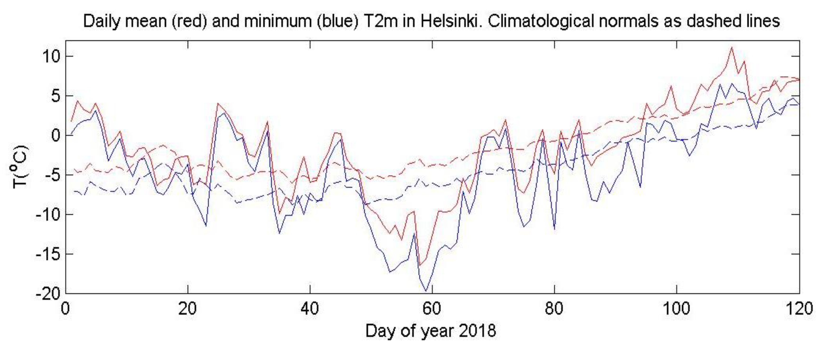
3. Surface Weather Response

The movement of the SPV over North America in February 2018 set up a tropospheric ridge/trough height field with cold temperatures over Central and Eastern Canada and the United States [5]. This persisted for most of February and was particularly evident in the second half of the month. The 850 hPa tropospheric vortex is co-located under the SPV center near Hudson Bay (Figure 1A and Figure 4). Cold temperature anomalies of <−8 °C reached well into the United States Midwest and were associated with strong cold air advection from the Arctic between the ridge over Alaska and the tropospheric vortex center.

The late-February European case is more complex [3]. While the main SPV was located over North America, it was nearly nonexistent over Europe (Figure 1A and Figure 2A); this allowed a region of tropospheric high pressure to build over Eurasia and spread westward over Northern Scandinavia and the Barents Sea associated with an anomalous weak SPV over Europe (Figure 1A and Figure 5). Cold air spread from Russia to the United Kingdom with snow falling as far south as Rome. Helsinki’s low temperatures of below −14 °C persisted for more than a week (Figure 6), while on 1 March many UK locations recorded their coldest March day in many decades [31], as the “Beast from the East” took hold. Several authors have noted in similar SSW cases that the persistence of the atmospheric structure was prolonged due to tropospheric/stratospheric interactions in both directions [6,20,32].

By mid-March the SPV was firmly over Eurasia (Figure 1D and Figure 2B). The stratospheric/tropospheric vortex connection was established and high pressure developed over the Atlantic (Figure 7). This pattern gave cold air advection from the Arctic over Europe. The cold event at Helsinki around day 80 (20 March) was not as pronounced as that in late February, as the region of coldest air was smaller and its movement was more progressive across Western Europe.

Although the stratospheric forcing on the evolution of surface weather location and intensity in February–March 2018 appears robust, we cannot exclude the potential role of other forcing factors. Although daily extremes of GBI and NAO occurred, February and March, 2018, were not exceptional in terms of monthly mean values of AO, NAO, and GBI. However, in 2018 the Tropical/Northern Hemisphere (TNH) pattern [33] reached its highest February mean value in the record starting from 1950, calculated by the NOAA Climate Prediction Centre [34]. A comparison of the three Februaries with largest monthly mean TNH values (2018, 1964, 2003) did not reveal a systematic spatial pattern of Northern Hemisphere surface air temperature anomalies.

In March 2018, the East Atlantic/West Russia (EA–WR) pattern [35,36] obtained its record-high value. The record-low March value of EA–WR occurred in 1970. The surface temperature anomalies showed similarities between 1970 and 2018: cold in Central Europe and Siberia, and warm in Alaska and Labrador–Southern Greenland region. Hence, although the study period was characterized by extreme values of TNH and EA–WR, we found no evidence of their having a major role for the “Beast from the East”.

4. Conclusions

There is considerable public interest on extreme weather events in midlatitudes that have a connection to the subarctic. Such events have been more frequent in the last decade [3,4,5], but to what degree that they are caused by recent changes in Arctic amplification is an open question [37]. A delay of sea ice formation during early winter in the Barents and Chukchi Seas is a potential forcing mechanism of the beginning of 2018 “Beast from the East” cold-air event and analogous events, but there is controversy about causality in the atmospheric community [9]. Other possible remote drivers of the closely-related SSW include mid-/high-latitude blocking and the Madden–Julian Oscillation [14]. The main dynamic factors for the “Beast from the East” severe weather were, however, internal variability of the SPV and tropospheric connections.

Late in winter there often is a subarctic-midlatitude weather connection related to the dynamics of the SPV. February–March 2018, show two types of connections. Mid-February and late-March are examples of vertically coherent geopotential height structures related to the displacement of the SPV over the two continents, and advection of cold Arctic air southward. The second type was exemplified after the SSW event of 12 February, 2018, in a region of weakened SPV over Northern Europe. These case studies show linkages between the Arctic SPV and midlatitude extreme weather based on internal variability of the polar atmosphere.

References

1. Waugh, D.W.; Sobel, A.H.; Polvani, L.M. What is the polar vortex and how does it influence weather? Bull. Am. Meteorol. Soc. 2017, 98, 37–44. [Google Scholar] [CrossRef]
2. Kidston, J.; Scaife, A.A.; Hardiman, S.C.; Mitchell, D.M.; Butchart, N.; Baldwin, M.P.; Gray, L.J. Stratospheric influence on tropospheric jet streams, storm tracks and surface weather. Nat. Geosci. 2015, 8, 433–440. [Google Scholar] [CrossRef]
3. Kretschmer, M.; Cohen, J.; Matthias, V.; Runge, J.; Coumou, D. The different stratospheric influence on cold-extremes in Eurasia and North America. Nat. Clim. Atmos. Sci. 2018, 1, 44. [Google Scholar] [CrossRef] [Green Version]
4. Cohen, J.; Pfeiffer, K.; Francis, J.A. Warm Arctic episodes linked with increased frequency of extreme winter weather in the United States. Nat. Commun. 2018, 9, 869. [Google Scholar] [CrossRef]
5. Overland, J.E.; Wang, M. Impact of the winter polar vortex on greater North America. Int. J. Climatol. 2019, 39, 5815–5821. [Google Scholar] [CrossRef] [Green Version]
6. King, A.D.; Butler, A.H.; Jucker, M.; Earl, N.O.; Rudeva, I. Observed relationships between sudden stratospheric warmings and European climate extremes. J. Geophys. Res. Atmos. 2019, 124, 13943–13961. [Google Scholar] [CrossRef]
7. Greening, K.; Hodgson, A. Atmospheric analysis of the cold late February and early March 2018 over the UK. Weather 2019, 74, 79–85. [Google Scholar] [CrossRef]
8. Cohen, J.; Screen, J.A.; Furtado, J.C.; Barlow, M.; Whittleston, D.; Coumou, D.; Francis, J.; Dethloff, K.; Entekhabi, D.; Overland, J.; et al. Recent Arctic amplification and extreme mid-latitude weather. Nat. Geosci. 2014, 7, 627–637. [Google Scholar] [CrossRef] [Green Version]
9. Nakamura, T.; Yamazaki, K.; Sato, T.; Ukita, J. Memory effects of Eurasian land processes cause enhanced cooling in response to sea ice loss. Nat. Commun. 2019, 10, 5111. [Google Scholar] [CrossRef] [PubMed] [Green Version]
10. Kalnay, E.; Kanamitsu, M.; Kistler, R.; Collins, W.; Deaven, D.; Gandin, L.; Iredell, M.; Saha, S.; White, G.; Woollen, J.; et al. The NCEP/NCAR 40-year reanalysis project. Bull. Am. Meteorol. Soc. 1996, 77, 437–471. [Google Scholar] [CrossRef] [Green Version]
11. Baldwin, M.P.; Dunkerton, T.J. Stratospheric harbingers of anomalous weather regimes. Science 2001, 294, 581–584. [Google Scholar] [CrossRef] [PubMed]
12. Charlton, A.J.; Polvani, L.M. A new look at stratospheric sudden warmings. Part I: Climatology and modeling benchmarks. J. Clim. 2007, 20, 449–469. [Google Scholar] [CrossRef]
13. Seviour, W.M.J.; Gray, L.J.; Mitchell, D.M. Stratospheric polar vortex splits and displacements in the high-top CMIP5 climate models. J. Geophys. Res. Atmos. 2016, 121. [Google Scholar] [CrossRef] [Green Version]
14. Karpechko, A.Y.; Charlton-Perez, A.; Balmaseda, M.; Tyrrell, N.; Vitart, F. Predicting sudden stratospheric warming 2018 and its climate impacts with a multimodel ensemble. Geophys. Res. Lett. 2018, 45, 13538–13546. [Google Scholar] [CrossRef] [Green Version]
15. Lee, S.H.; Butler, A.H. The 2018–2019 Arctic stratospheric polar vortex. Weather 2020, 75, 52–57. [Google Scholar] [CrossRef]
16. Hoskins, B.J.; McIntyre, M.E.; Robertson, A.W. On the use and significance of isentropic potential vorticity maps. Q. J. R. Meteorol. Soc. 1985, 111, 877–946. [Google Scholar] [CrossRef]
17. Thompson, D.W.J.; Baldwin, M.P.; Wallace, J.M. Stratospheric connection to Northern Hemisphere wintertime weather: Implications for prediction. J. Clim. 2002, 15, 1421–1428. [Google Scholar] [CrossRef]
18. Hitchcock, P.; Simpson, I.R. The downward influence of stratospheric sudden warmings. J. Atmos. Sci. 2014, 71, 3856–3876. [Google Scholar] [CrossRef]
19. Kautz, L.-A.; Polichtchouk, I.; Birner, T.; Garny, H.; Pinto, J.G. Enhanced extended-range predictability of the 2018 late-winter Eurasian cold spell due to the stratosphere. Q. J. R. Meteorol. Soc. 2020, 146, 1040–1055. [Google Scholar] [CrossRef] [Green Version]
20. Butler, A.H.; Sjoberg, J.P.; Seidel, D.J.; Rosenlof, K.H. A sudden stratospheric warming compendium. Earth Syst. Sci. Data 2017, 9, 63–76. [Google Scholar] [CrossRef] [Green Version]
21. Dee, D.P.; Uppala, S.M.; Simmons, A.J.; Berrisford, P.; Poli, P.; Kobayashi, S.; Andrae, U.; Balmaseda, M.A.; Balsamo, G.; Bauer, P.; et al. The ERA-Interim reanalysis: Configuration and performance of the data assimilation system. Q. J. R. Meteorol. Soc. 2011, 137, 553–597. [Google Scholar] [CrossRef]
22. Climate Prediction Center, National Weather Service. Available online: https://www.cpc.ncep.noaa.gov/ (accessed on 7 May 2020).
23. Masato, G.; Hoskins, B.J.; Woollings, T.J. Wavebreaking characteristics of midlatitude blocking. Q. J. R. Meteorol. Soc. 2012, 138, 1285–1296. [Google Scholar] [CrossRef]
24. Woollings, T.; Barriopedro, D.; Methven, J.; Son, S.-W.; Martius, O.; Harvey, B.; Sillmann, J.; Lupo, A.R.; Seneviratne, S. Blocking and its response to climate change. Curr. Clim. Chang. Rep. 2018, 4, 287–300. [Google Scholar] [CrossRef] [PubMed] [Green Version]
25. Hanna, E.; Hall, R.J.; Cropper, T.E.; Ballinger, T.J.; Wake, L.; Mote, T.; Cappelen, J. Greenland Blocking Index daily series 1851–2015: Analysis of changes in extremes and links with North Atlantic and UK climate variability and change. Int. J. Climatol. 2018, 38, 3546–3564. [Google Scholar] [CrossRef]
26. Strong, C.; Magnusdottir, G. Tropospheric Rossby wave breaking and the NAO/NAM. J. Atmos. Sci. 2008, 65, 2861–2876. [Google Scholar] [CrossRef]
27. Kunz, T.; Fraedrich, K.; Lunkeit, F. Impact of synoptic-scale wave breaking on the NAO and its connection with the stratosphere in ERA-40. J. Clim. 2009, 22, 5464–5480. [Google Scholar] [CrossRef]
28. Aikawa, T.; Inatsu, M.; Nakano, N.; Iwano, T. Mode-decomposed equation diagnosis for atmospheric blocking development. J. Atmos. Sci. 2019, 76, 3151–3167. [Google Scholar] [CrossRef]
29. Huang, J.; Tian, W.; Gray, L.J.; Zhang, J.; Li, Y.; Luo, J.; Tian, H. Preconditioning of Arctic stratospheric polar vortex shift events. J. Clim. 2018, 31, 5417–5436. [Google Scholar] [CrossRef]
30. Tao, W.; Zhang, J.; Zhang, X. The role of stratosphere vortex downward intrusion in a long-lasting late-summer Arctic storm. Q. J. R. Meteorol. Soc. 2017, 143, 1953–1966. [Google Scholar] [CrossRef]
31. Galvin, J.; Kendon, M.; McCarthy, M. Snow cover and low temperatures in February and March 2018. Weather 2019, 74, 104–110. [Google Scholar] [CrossRef]
32. Lu, C.H.; Ding, Y.H. Observational responses of stratospheric sudden warming to blocking highs and its feedbacks on the troposphere. Chin. Sci. Bull. 2013, 58, 1374–1384. [Google Scholar] [CrossRef] [Green Version]
33. Mo, K.C.; Livezey, R.E. Tropical-extratropical geo-potential height teleconnections during the Northern Hemisphere winter. Mon. Wea. Rev. 1986, 114, 2488–2515. [Google Scholar] [CrossRef]
34. Tropical Northern Hemisphere (TNH), NOAA Climate Prediction Center. Available online: https://www.cpc.ncep.noaa.gov/data/teledoc/tnh.shtml (accessed on 7 May 2020).
35. Barnston, A.G.; Livezey, R.E. Classification, seasonality and persistence of low-frequency atmospheric circulation pattern. Mon. Weather Rev. 1987, 115, 1083–1126. [Google Scholar] [CrossRef]
36. Ionita, M. The impact of the East Atlantic/Western Russia pattern on the hydroclimatology of Europe from mid-winter to late spring. Climate 2014, 2, 296–309. [Google Scholar] [CrossRef] [Green Version]
37. Francis, J.A.; Skific, N.; Vavrus, S.J. North American weather regimes are becoming more persistent: Is Arctic amplification a factor? Geophys. Res. Lett. 2018, 45, 11414–11422. [Google Scholar] [CrossRef] [Green Version]
Figure 1. A 100 hPa geopotential height field (m, heights indicated by isolines and anomalies by color shadings relative to a 1981–2010 base period) for selected sub-periods from February–March 2018. Data are from NCEP–NCAR reanalysis.
Atmosphere 11 00664 g001
Figure 2. Potential vorticity (PV) at 315 K isentropic surface during (A) 5–23 February and (B) 4–31 March, 2018. The unit is PVU (1.0 PVU = 10−6 K kg−1 m2 s−2). In climatology, the 315 K isentropic surface extends from the lower stratosphere in the Arctic region to the mid-troposphere in the sub-Arctic or midlatitudes.
Atmosphere 11 00664 g002
Figure 3. (a) Daily anomalies of 100 hPa meridional eddy heat flux averaged over 45–75° N, [v’T’]. (b) The Northern Annular Mode (NAM) index at different atmospheric levels, calculated as the inverse of the standardized polar cap geopotential height anomaly averaged over 65–90° N. (c) Vortex aspect ratio and centroid latitude and (d) the NAO and AO indices for winter 2017–2018. Filled circles denote periods of at least 7 consecutive days when the vortex moment threshold is crossed. NAM and vortex moments use ERA–Interim data [21] and the AO and NAO indices are from NOAA Climate Prediction Center [22].
Atmosphere 11 00664 g003
Figure 4. Composite of atmospheric 850 hPa geopotential height (contours in units of meters) and temperature anomaly fields (color shading relative to a 1981–2010 base period) for 5–23 February 2018. Data are from NCEP–NCAR reanalysis.
Atmosphere 11 00664 g004
Figure 5. Composite of atmospheric 850 hPa geopotential height (contours in units of m) and temperature anomaly fields (color shading) for 24–27 February 2018. Data are from NCEP–NCAR reanalysis.
Atmosphere 11 00664 g005
Figure 6. Helsinki daily mean and minimum temperature for early 2018 relative to the climatology averaged over 1981–2010. Data from Finnish Meteorological Institute.
Atmosphere 11 00664 g006
Figure 7. Composite of atmospheric 850 hPa geopotential height (contours, in units of m) and temperature anomaly fields (color shading) for 15–20 March 2018. Data are from NCEP–NCAR reanalysis.
Atmosphere 11 00664 g007