1. Introduction
The characteristics of the convective boundary layer (CBL), a type of planetary boundary layer (PBL) in which surface buoyancy flux drives turbulence, exhibit a strong dependency on surface and atmospheric forcings. For instance, the organization of turbulent circulations in the CBL is controlled by the interplay between buoyancy and wind shear. When surface buoyancy flux is large relative to wind shear, convective cells composed of central downdrafts and narrow circumferential updrafts appear like the Rayleigh–Bénard convection [
1,
2]. In contrast, when wind shear dominates over the surface buoyancy flux, convective rolls, pairs of linear up- and downdrafts appear, and they are typically aligned 10–20
to the left of mean wind direction in the Northern Hemisphere [
2,
3,
4,
5]. The characteristics of the two extreme and intermediate CBLs have been successfully investigated by using turbulent eddy-resolving models such as a large-eddy simulation (LES) model (see the discussions and references in [
6]). For example, Khanna and Brasseur [
7] simulated five CBLs in a range of
from 0.44 to 730, where
h and
L are the PBL depth and the Obukhov length, respectively. The stability parameter
indicates the relative roles of shear and buoyancy in the production/consumption of turbulent kinetic energy (TKE) in the PBL [
8], and Khanna and Brasseur [
7] demonstrated that various convective flow structures appear depending on the stability. Recently, Salesky et al. [
6] simulated CBLs in a wider range of
and found that the transition between the convective rolls and cells occurs gradually but a significant change in their organization occurs at
15–20. The transition of the CBL organization has been reported to affect the efficiency of momentum and heat transport [
6], and the transition can affect moisture transport and thus the mass flux of shallow cumulus convection [
9]. Furthermore, coherent perturbations especially in the convective rolls are able to influence the initiation of deep cumulus convection [
10,
11].
The CBL over land decays as the surface buoyancy flux decreases in the afternoon and evening. Especially near sunset, the CBL quickly transitioned to a residual layer and a stable boundary layer below. This so-called evening transition is accompanied by temperature drop, humidity jump, and wind speed decrease near the surface [
12]. The abrupt transition of the CBL has been investigated through field observations, laboratory experiments, theoretical models, and eddy-resolving model simulations (see the reviews by [
13,
14]). Important features of the transition are that the CBL undergoes slow decay first and then faster decay and nonlocal eddies control the decay process. Nieuwstadt and Brost [
15] performed very simplified CBL simulations in which surface heat flux is suddenly cut off. They discovered that the vertically averaged TKE stays constant for a period of
, where
is the convective velocity scale [
16], and then decreases following a power law. Sorbjan [
17] simulated a similar decaying CBL but forced by gradually decreasing surface heat flux. The decay of the CBL was shown to be controlled by two scales, the convective time scale
and the external time scale of surface heat flux change. In his simulation, nonlocal eddies persist even when the surface heat flux becomes negative. Darbieu et al. [
18] used more realistic forcing (e.g., observed surface fluxes and simulated mesoscale advection) in simulating the decaying CBLs observed in the Boundary Layer Late Afternoon and Sunset Turbulence (BLLAST) field study, and the simulated results (e.g., evolution of TKE) were similar to the observations. Pino et al. [
19] investigated the decay of convective turbulence focusing on the impacts of wind shear and inversion strength. They performed a set of four simulations and found that wind shear delays the decay. The delay of the CBL decay was confirmed in the theoretical model results of [
20]. Recently, the delay was reconfirmed in Park and Baik [
21], who simulated free and advective decaying CBLs. They insisted that unsustainable circulations, cool updrafts and warm downdrafts observed in the free decaying CBL, accelerate the decay of convective turbulence and the unsustainable circulations are hardly detectable in the advective decaying CBL maybe due to stronger wind shear. However, the mechanism explaining how wind shear delays the decay of the CBL is not completely understood. Furthermore, the simulations in [
19,
21] are limited to a narrow range of stability. Thus, a more systematic investigation is required to reveal the role of wind shear in the decay of CBLs in a wider range of stability.
The main objective of this study is to investigate how wind shear affects the decay of the CBL. We perform nine numerical simulations with varying magnitudes of geostrophic wind and surface sensible heat flux, thus covering weakly to strongly convective boundary layers, and we investigate their decaying phases after the surface heat flux is suddenly stopped. We describe the LES model and the simulation setup in
Section 2. The simulation results are presented and discussed in
Section 3, and a summary and conclusions are given in
Section 4.
2. Model Description and Setup
The parallelized LES model (PALM) version 6.0 [
22] is used to simulate growing and suddenly decaying CBLs. The nicely parallelized LES model explicitly resolves turbulent eddies of interest and parameterizes only subgrid-scale fluxes based on the inertial subrange theory. Thus, the model can accurately simulate energy-containing eddies in urban surface layers, PBLs, and cloud layers using affordable computing resources, and it has been widely used and validated (see the references in [
23]). The PALM solves the implicitly filtered Navier–Stokes equations of velocity components
u,
v,
w, potential temperature
, and subgrid-scale TKE on the staggered Arakawa C-grid [
24]. The model used in this study employs the Boussinesq approximation, and temporal and spatial integrations are done using a third-order Runge–Kutta scheme [
25] and an upwind-biased 5th-order scheme [
26], respectively. The 1.5-order Deardorff [
27] scheme is used for the parameterization of subgrid-scale fluxes.
Nine CBL simulations considering three different geostrophic wind speeds and three different surface heat fluxes are performed. The characteristics of the 9 well-developed CBLs are presented in
Table 1. The geostrophic winds in the
x (west-east) direction are 0.1, 5, and 10 m s
in buoyancy-dominated B1–3, intermediate I1–3, and strong-shear S1–3 cases, respectively. The geostrophic wind in the
y (south-north) direction is 0 m s
in all the cases. The numbers in the case names indicate the magnitudes of surface sensible heat flux, and the surface heat flux varies from 0.1 to 0.3 K m s
. Each experiment is simulated for 6 h, and the surface sensible heat flux is implemented until the cutoff time
(
t = 3 h) and then stopped. The grid size in the
x and
y directions is 20 m, and the grid size in the
z (vertical) direction is 20 m below
z = 1.2 km and gradually increased to 50 m above
z = 1.2 km. The computation domain of
km
is covered by
grid boxes. Above
z = 1.7 km, the Rayleigh damping is implemented to damp gravity waves reflected from the top boundary. The initial potential temperature is 300 K below
z = 0.7 km and increases upward with a lapse rate of 10 K km
above that level. The Coriolis force at 37
N is implemented, and it turns mean wind direction in the clockwise direction upward in the boundary layers. The time step, being dynamically determined to satisfy the Courant–Friedrichs–Lewy condition, ranges from 3.3 s to 20 s. Turbulent statistics are calculated every ∼10 s, and three-dimensional data are sampled every ∼60 s for more analysis.
3. Results and Discussion
The combination of three different geostrophic wind speeds and three different surface heat fluxes enables the simulation of CBLs in a wide range of stability. We calculate the dimensionless stability parameter
, and it ranges from 5.7 to 363.7 at
, corresponding to weakly and strongly convective regimes, respectively (
Table 1). In this study, we define the PBL depth
h as the horizontal average of levels where maximum vertical gradient of potential temperature occurs [
28]. The PBL depth can be defined in a different way as the level of minimum heat flux
, and
is lower than
h by 40–80 m (
Table 1). The PBL depth increases with increasing surface heat flux. The convective velocity scale
is defined as
, where
g and
are the gravitational acceleration and the potential temperature at the lowest model level, and it represents the magnitude of boundary layer convection. The convective velocity scale increases with increasing surface heat flux, too. The convective time scale
in this study is defined as
, where
is the convective velocity scale considering the impact of surface wind shear [
29,
30]. The modified convective velocity scale is defined as [
19]:
Here,
represents the friction velocity and the friction velocity increases with increasing geostrophic wind speed. The friction velocity slightly increases with increasing surface heat flux, too, and this is because larger surface heat flux induces stronger circulations and larger wind shear near the surface. The difference of
between the same
cases (e.g., B1–3 cases) decreases over time as convective turbulence decays, and the friction velocities in the buoyancy-dominated cases are almost the same at the end of the 6-h simulation (
Table 2).
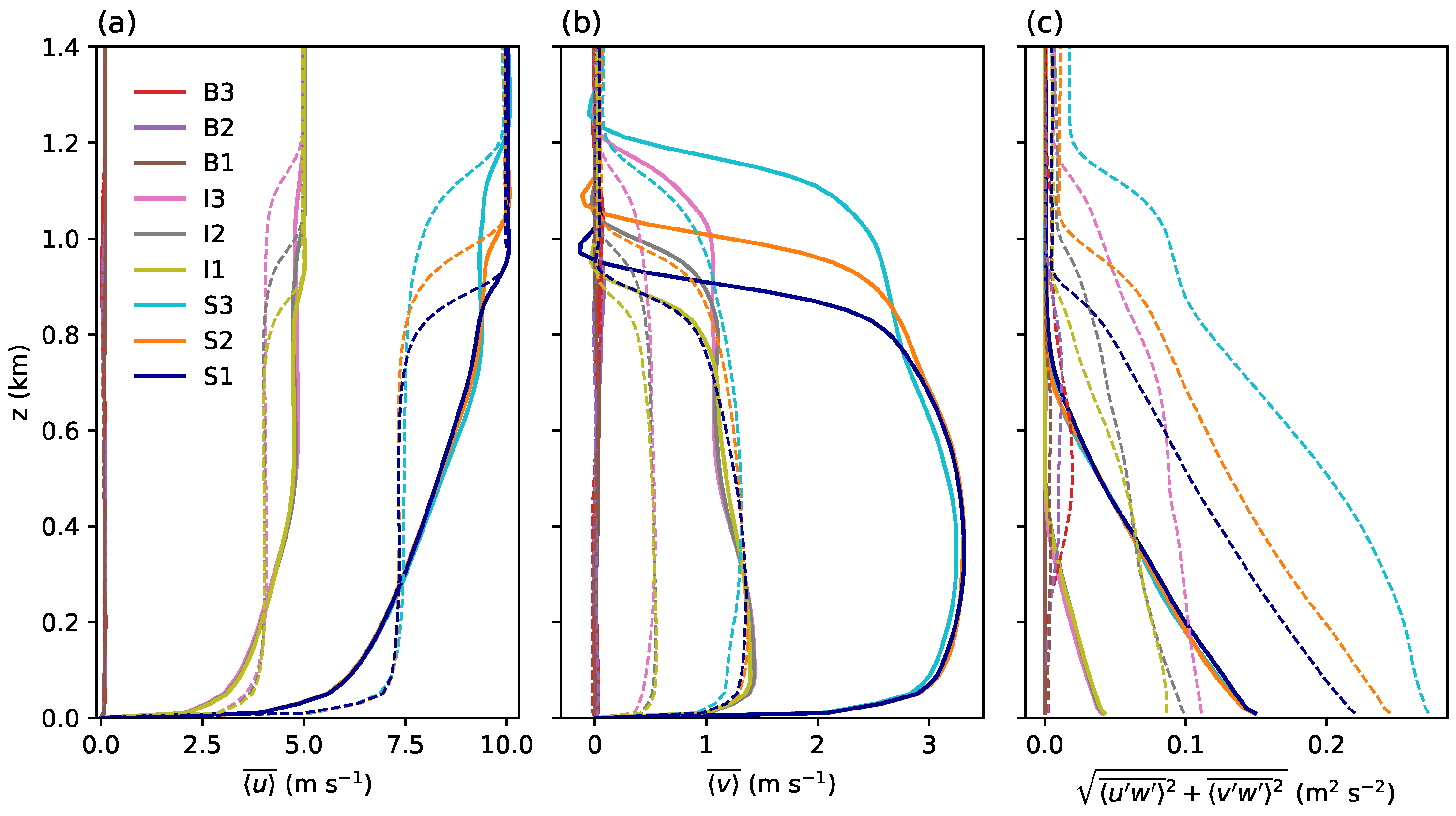
The deepening of PBL following the strength of surface thermal forcing is observed again in the vertical profiles of temporally and horizontally averaged horizontal velocities
and
and vertical turbulent momentum flux
(
Figure 1). In this study, overbars and angle brackets indicate temporal (600 s) and horizontal averages, respectively, and primes denote horizontal perturbations. The 6 CBLs in the I1–3 and S1–3 cases are grouped according to mean wind velocity and PBL depth. The PBL depth can be estimated from the depth of uniform-wind-layer, and it increases with increasing surface heat flux at
(
Figure 1a,b). The
x- and
y-directional mean wind velocities in the 6 CBLs are determined by the geostrophic wind of each case. After the cutoff of surface heat flux, the well-mixed boundary layers are transitioned to residual layers and the vertical gradient of the
x-directional velocity increases except near the surface and the PBL top. The
y-directional velocity does not show the vertically increasing pattern, but it increases over time until the end of the 6-h simulation (
Figure 1b). The temporal increase is attributable to the Coriolis force, accelerating
v when
u is smaller than
, and the increase stops in a supergeostrophic wind condition (after
t = 6 h, not shown). The vertical turbulent momentum fluxes at
in the 6 cases decrease upward, and their magnitudes show a dependency on the geostrophic wind speed and the surface heat flux. After 3 h, the dependency on the surface heat flux disappears and the momentum flux profiles collapse to three groups depending on the geostrophic wind speed. In contrast to the above 6 cases, the mean wind velocities and the vertical turbulent momentum fluxes in the (buoyancy-dominated) B1–3 cases are very small and the differences between the B1–3 cases are not detectable in their vertical profiles.
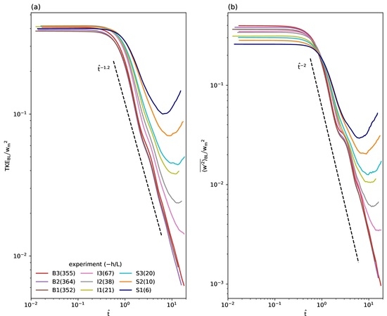
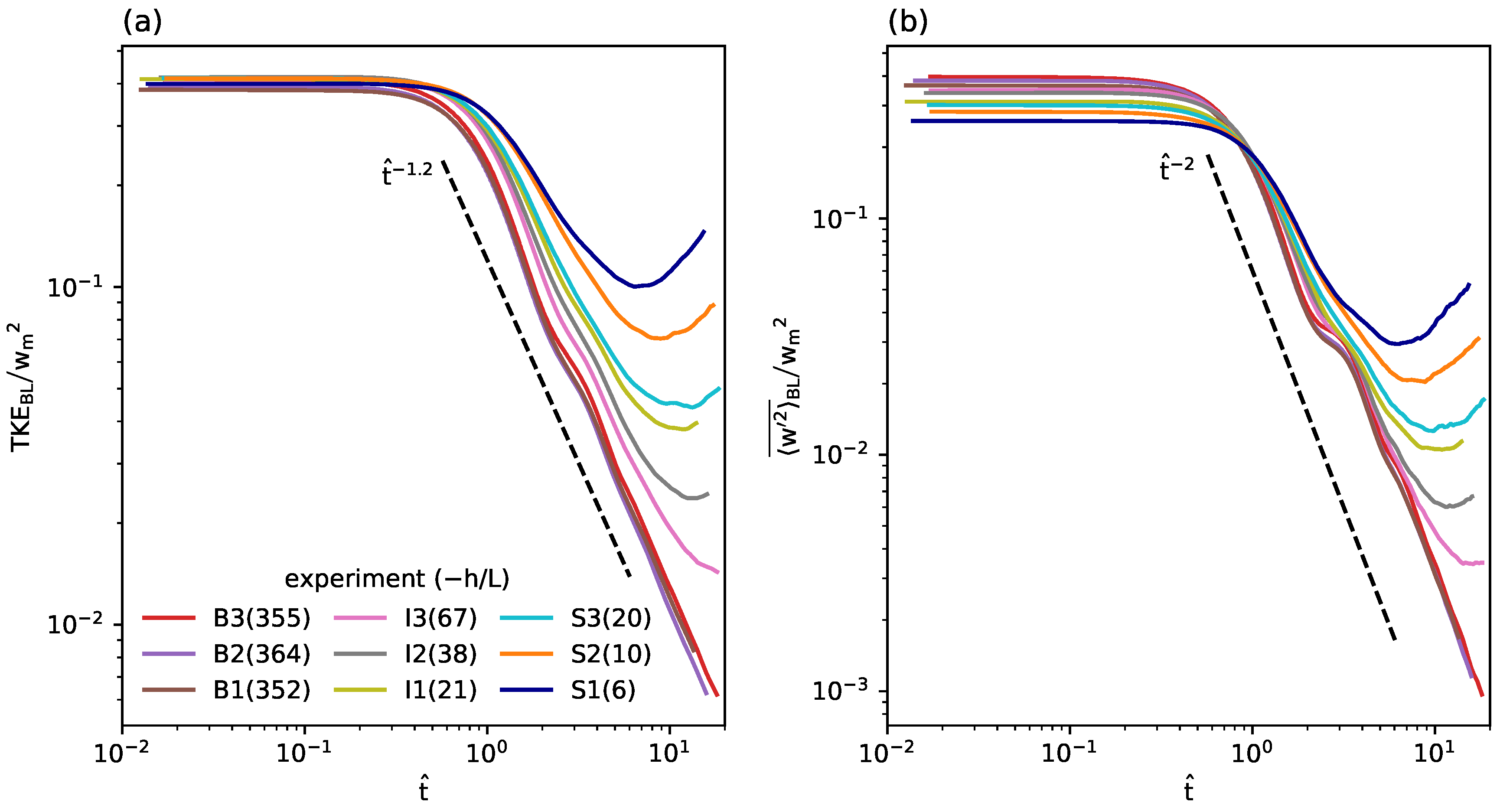
Figure 2 shows the time series of the normalized and boundary-layer-averaged TKE and vertical velocity variance. For the comparison of 9 CBLs, the TKE and vertical velocity variance are vertically averaged below
and then divided by
, and the results are finally represented as functions of the dimensionless time
. The initial level of TKE is maintained for a period of one convective time scale. Then, convective turbulence decays following a power law and the exponent is approximately −1.2 as the value in [
15]. While the TKEs of the B1–3 cases decrease monotonically until the end of the simulation, the TKEs of the I1–3 and S1–3 cases decrease much slower or even increase in the later period. After
, the vertical velocity variances decrease following a power law, too, and the exponent is close to −2 as the value in [
15]. In the I1–3 and S1–3 cases, the vertical velocity variances decrease slower than the B1–3 cases and the variances increase in the later period especially in the I1–2 and S1–3 cases (
37.7). The normalized and vertically averaged variances of
u and
v decrease slower with stronger wind shear, too (not shown). The slower decay of turbulence in the strong-shear CBLs than in the buoyancy-dominated CBLs was reported in [
19], but the increase of turbulence in the later period was not observed in their simulations. We speculate that the increase of turbulence in their simulations may be delayed due to a different experiment setup and thus not be detected in their shorter-period (2-h) simulations.
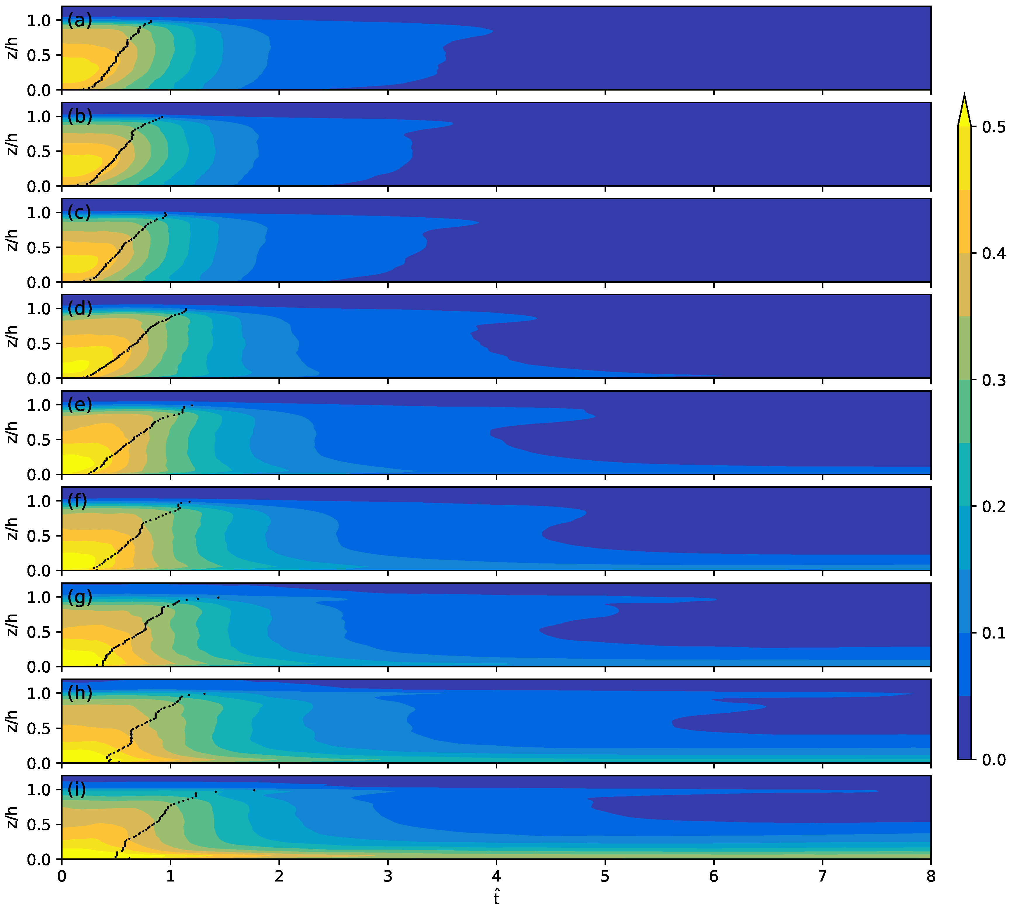
The time series of normalized TKE profiles are presented in
Figure 3. We normalize TKEs by dividing them by
. In the B1–3 cases, maximum of TKE occurs below the middle of PBL (e.g.,
) at
and the maximum level rises as convective turbulence decays, thus maximum of TKE occurs above the middle of PBL after a period of one convective time scale. As wind shear becomes stronger with respective to surface heat flux, maximum of TKE occurs at lower level and the near-surface TKE decays more slowly or even increases. For example, a significant level of TKE is maintained until the end of the simulation in the I1 and S1–3 cases. It seems that mechanically generated eddies near the surface overcome the initial decay and the following weakly but stably stratified environment.
To illustrate the overall vertical circulations, normalized vertical velocities in PBLs (below
) are averaged and the vertically averaged
fields in the B3, I2, and S1 cases are presented in
Figure 4. We select these three cases because they represent the buoyancy-dominated , intermediate , and strong wind-shear cases well. In the B3 case, convection cells are clearly seen in the vertically averaged
fields at
and the cellular structures are observed at
(
Figure 4d) and even at
(
Figure 4g). It is remarkable that the cellular convections at
= 1 and 3 are out of phase. For example, the vertically averaged
at (
x,
y) = (2.23 km, 6.97 km) is positive at
= 1 and negative at
= 3 and vice versa at (
x,
y) = (2.23 km, 5.77 km). In the S1 case, convective rolls appear and decay over time (
Figure 4c,f,i), and local eddies replace them at
= 8 (
Figure 4l). Intermediate structures between the cells and rolls appear in the I2 case [
6], and they also decay over time. However, the reversal of vertically averaged
observed in the B3 case is hardly detectable in the same fields of the I2 and S1 cases. Thus, we expect that wind shear acts to block or disturb the reversal of vertical circulations.
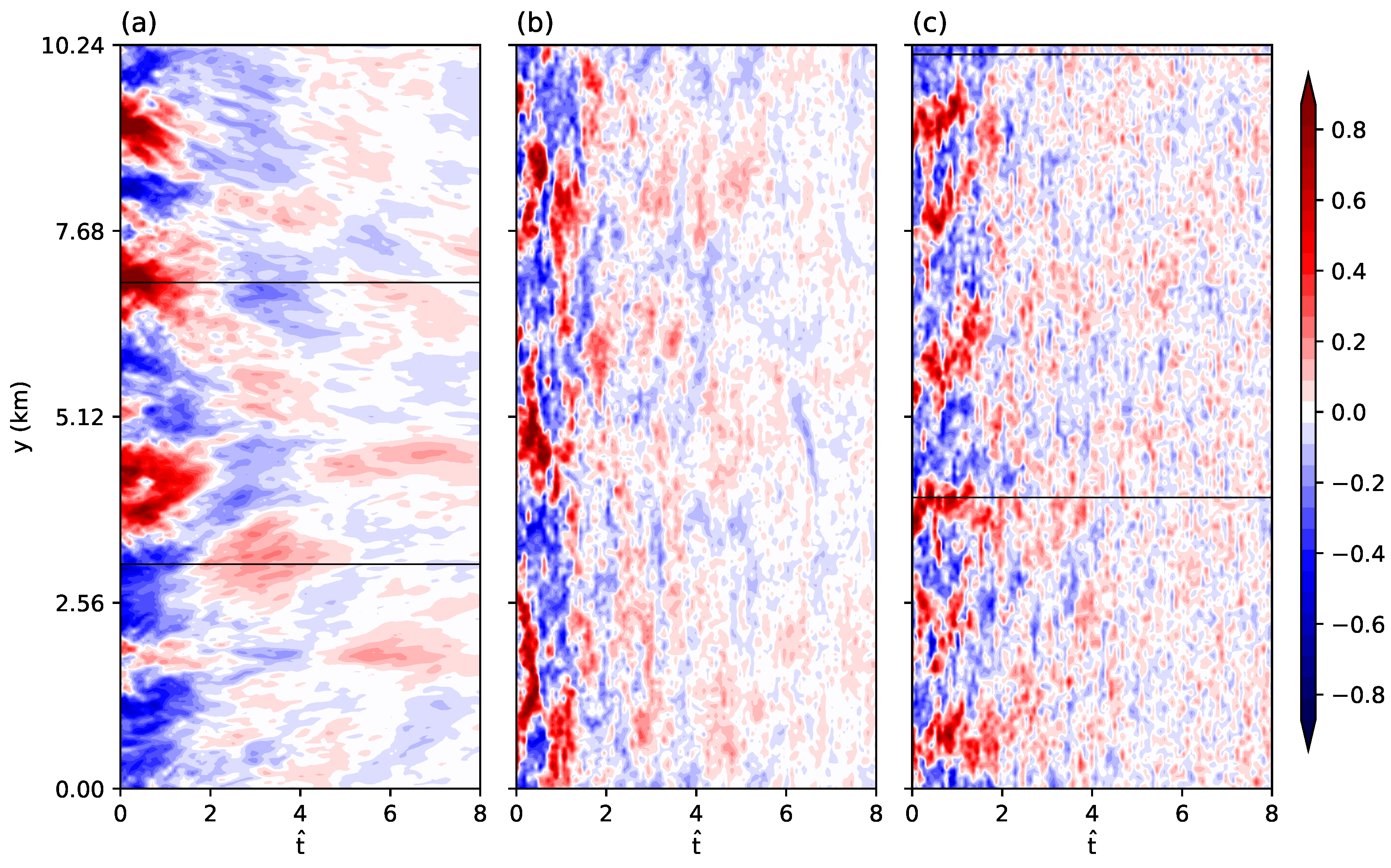
To illustrate more details of the boundary layer circulations, we present the time series of the normalized and vertically averaged vertical velocity at (
x,
y) = (2.23 km, 0–10.24 km) in
Figure 5. In the B3 case, the temporal reversal of vertically averaged
repeats along with the decay of turbulence. The existence of oscillations even in this smoothened vertical velocity field indicates that boundary-layer scale oscillations exist. The time series of
profiles at the two points (
x,
y) = (2.23 km, 6.97 km) and (2.23 km, 3.09 km) confirm the oscillations again, but the oscillations become weak and local after a period of several
(
Figure 6a,b). The oscillations are not distinct in the I2 and S1 cases. In the two cases, convective structures decay and move eastward simultaneously, and thus pure temporal changes of
are hardly detectable in the time series at fixed locations (
Figure 5b,c). The time series of
profiles in
Figure 6c,d demonstrate again that turbulent eddies in the S1 case are more complex than those in the B3 case.
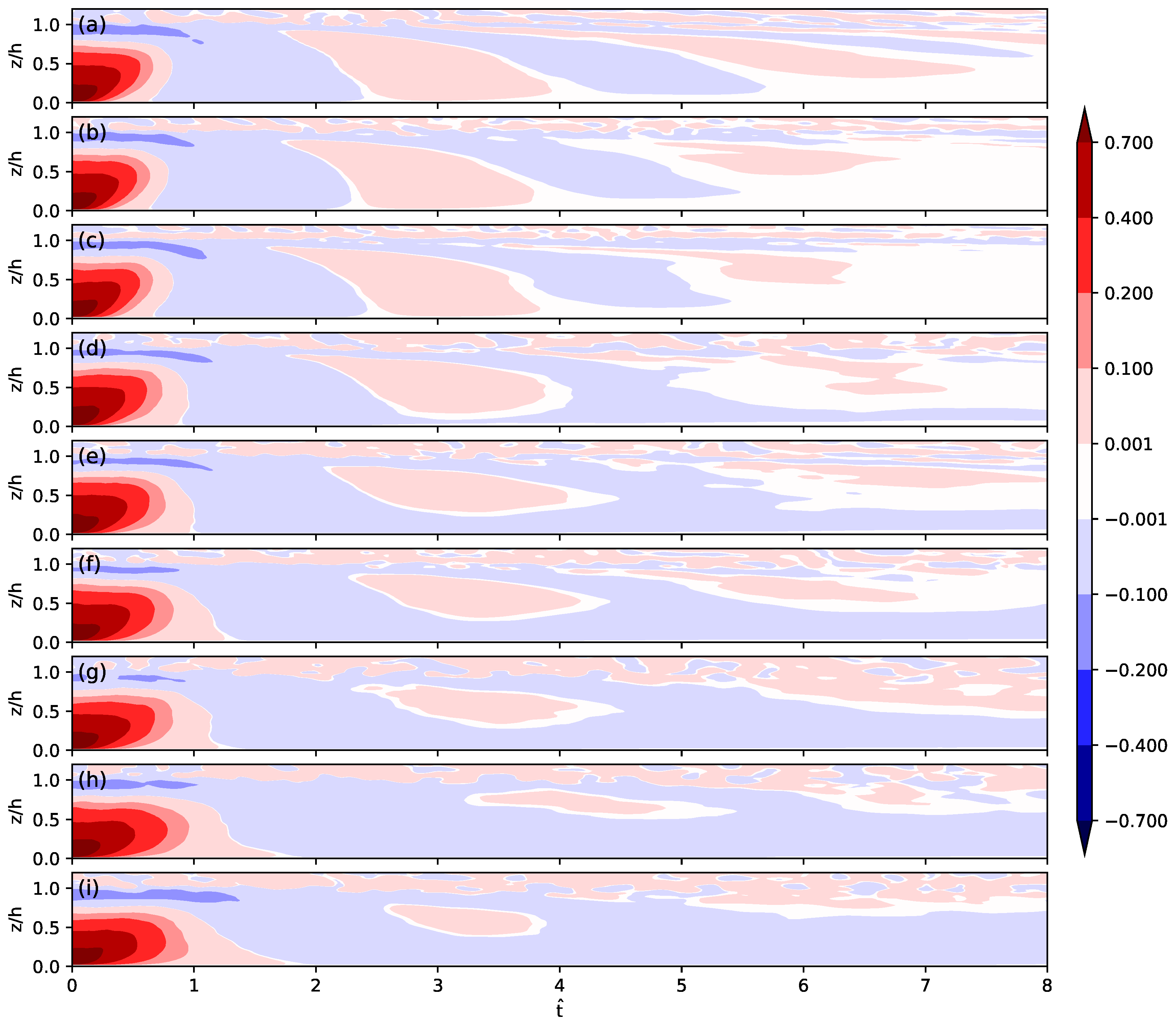
The time series of normalized vertical turbulent heat flux profiles in
Figure 7 demonstrate that the oscillation of vertical velocity induces an oscillation of heat flux in the B1–3 cases. The vertical turbulent heat fluxes are normalized by dividing by
. The vertical range of the oscillation becomes narrower over time and thus vertical heat transport is not significant any more later in the lower residual layer in the B1–3 cases, as indicated by white shading in the later period in
Figure 7a–c. In the other cases, however, the oscillation of heat flux is not distinct. Instead, the negative heat flux across the PBL after
becomes positive locally near the middle of PBL but for a short time (<
). Another remarkable feature is that the positive to negative transition of vertical heat flux in the lower PBL (e.g., below
) starts from the bottom surface in the B1–3 and I2–3 cases. In the I1 and S1–3 cases, however, the bottom-up transition seems to be blocked by near-surface eddies and the negative heat flux seems to be gradually propagating downward from above. Especially near the surface in the I1 and S1–3 cases, turbulent eddies transport heat downward all through the simulation period after the heat flux becomes negative from positive at
= 1.3–2 (
Figure 7f–i).
The joint probability density function (PDF) of potential temperature perturbation and normalized vertical velocity in
Figure 8 shows the vertical heat transport patterns in a different perspective. The joint PDF of two variables
A and
B at each bin center (
a,
b) is calculated using the expression:
Here,
and
are the bin widths of the variables
A and
B, respectively. We collect sufficient data at three levels (
= 0.23, 0.25, and 0.27) and calculate the joint PDFs using
bins at
= 0, 1, 2, 3, 5, and 8. The contours of 0.1 are plotted, and the value 0.1 is selected to visualize the distribution of representative events in the B3 and S1 cases as the best as we can. The joint PDF at
= 0 in the B3 case indicates that warm updrafts and cool downdrafts maintain the cellular convection and a similar but less stretched distribution appears in the S1 case (
Figure 8a). Potential temperature perturbation and vertical velocity are positively correlated in the two cases, and this corresponds to the positive vertical heat fluxes at
= 0 and
in
Figure 7a,i. At
= 1, the diagonally stretched distribution in the B3 case becomes circular and it becomes more and more circular as time goes on. The circular and symmetric distribution corresponds to the negligible vertical heat flux at
in the later period of the B3 case (
Figure 7a). On the other hand, the joint PDF at
= 1 in the S1 case is still diagonally stretched, matching with the positive vertical heat flux at the same time in
Figure 7i. The joint PDF in the S1 case becomes vertically stretched over time with a weak bump of slightly warmer air after
= 2. The bump of weakly sinking warm air can be attributable to that upper-level warm air parcels are pulled downward by local downdrafts like the sporadic eddies in
Figure 4l, and thus the local downdrafts transport heat downward in the stably stratified environment. We conjecture that the negative vertical heat fluxes near the surface in the I1 and S1–3 cases are attributed to this kind of distributions driven by mechanical eddy circulations.
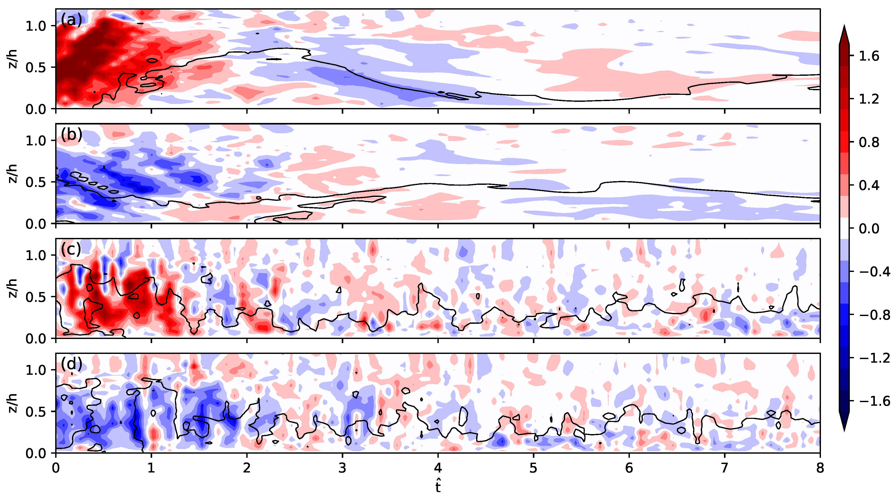
Figure 9 shows the time series of skewness (normalized third central moment) of vertical velocity
. At
= 0, a top-heavy profile of skewness is observed in all the cases and the skewness decays from the bottom up. The skewness of vertical velocity in the upper boundary layer is quite large for some time (e.g., larger than 0.8 for
= 0–0.5 in the B3 case) and then decays quickly as the boundary-layer-averaged TKE decays. However, the skewness near the surface decays right after the cutoff time. Especially in the B1–3 cases, the near-surface skewness becomes negative at
= 0.3–0.4 and a negative-skewness regime forms and extends upward at
= 2–3. This upward extension and later shrinkage seem to be related to the reversal of vertical circulations seen in
Figure 5a, and this indicates that downdrafts in the lower boundary layer play an important role in the decay of convective turbulence. In the S1–3 cases, the near-surface skewness decreases but much slower than in the B1–3 cases and small negative skewness is observed after a period of several convective time scales. The negative third moment of
w in the surface layer was reported in the neutral PBL simulated by Moeng and Sullivan [
29] but note that the small negative value can be erroneous due to missing subgrid vertical velocity variance [
31]. Right above the level of negative skewness, positive skewness of vertical velocity occurs and the positive-skewness regime extends upward over time in the S1–3 cases. The profiles of vertical velocity skewness in the I3 and I1 cases resemble the profiles in the buoyancy-dominated (B1–3) cases and those in the strong-shear (S1–3) cases, respectively, and quite intermediate profiles of vertical velocity skewness appear in the I2 case.


