Impact of Lidar Data Assimilation on Low-Level Wind Shear Simulation at Lanzhou Zhongchuan International Airport, China: A Case Study

Abstract

Doppler wind lidar has played an important role in alerting low-level wind shear (LLW). However, these high-resolution observations are underused in the model-based analysis and forecasting of LLW. In this regard, we employed the Weather Research and Forecasting (WRF) model and its three-dimensional variational (3D-VAR) system to investigate the impact of lidar data assimilation (DA) on LLW simulations. Eight experiments (including six assimilation experiments) were designed for an LLW process as reported by pilots, in which different assimilation intervals, assimilation timespans, and model vertical resolutions were examined. Verified against observations from Doppler wind lidar and an automated weather observing system (AWOS), the introduction of lidar data is helpful for describing the LLW event, which can represent the temporal and spatial features of LLW, whereas experiments without lidar DA have no ability to capture LLW. While lidar DA has an obviously positive role in simulating LLW in the 10–20 min after the assimilation time, this advantage cannot be maintained over a longer time. Therefore, a smaller assimilation interval is favorable for improving the simulated effect of LLW. In addition, increasing the vertical resolution does not evidently improve the experimental results, either with or without assimilation.

1. Introduction

Low-level wind shear (LLW), which is a known aviation safety hazard, is receiving more attention as the number of flights increases [1,2,3]. LLW generally takes place below 500 m and may be caused by certain mesoscale or microscale systems, such as thunderstorms, microbursts, and gust fronts [4,5]. When flights encounter LLW during takeoff or landing, the small temporal–spatial range of LLW occurrence makes pilots’ response difficult. Therefore, it is necessary to determine the timings and positions of LLW by numerical models or other effective methods.

Numerical weather prediction (NWP) technology is an effective tool for providing future weather information, and successful predictions on severe weather phenomena can reduce the damage to human lives and social resources [6]. Considering the small temporal–spatial scale and high variability of LLW, model-based simulation or forecasting should be performed at a high resolution (e.g., several kilometers or less). Some related studies that have been documented at present include ideal simulation experiments of terrain-induced turbulence [7], large-eddy simulation of the turbulent wake and its potential impact on low-level wind [8], a Lee wave case study over three-dimensional mountainous terrain [9], and numerical predictions (or simulations) on wind shear cases based on shallow-water models [10] or the Weather Research and Forecasting (WRF) model [11,12,13]. Furthermore, a systematic evaluation of LLW prediction was first performed through two-year NWP results at Hong Kong International Airport (HKIA), in which conventional upper-air and surface observations were assimilated into the operational aviation model [3]. The high-resolution NWP has a positive prediction skill for LLW, which can reproduce LLW features, but the predicted timing and position of LLW must be improved [3,11].

In general, LLW that occurs in non-rainy weather conditions may be more difficult to predict due to its complex mechanism than that which occurs in rainy conditions associated with the convection system [5,14]. Such LLW draws more attention [14,15]. Doppler wind lidar, as a new observational instrument for capturing this kind of LLW event, has been installed in many airports in recent years, including Hong Kong [14], Las Vegas [16], Nice [11], Tokyo [17], Beijing [18,19], and Lanzhou airports [15,20]. The wind information obtained from Doppler wind lidar has a fine temporal and spatial resolution (typically 50–200 m), which remains valuable and useful in LLW analysis in non-rainy regions [14,15,21].

To date, the applications of Doppler wind lidar in the detecting and alerting of LLW have been well-recognized [14,15,19,22]. However, lidar data have been insufficiently applied in the prediction of LLW, for example, by assimilating lidar data into NWP models. Recently, Kawabata et al. [23] evaluated the role of lidar data assimilation (DA) in predicting a mesoscale convective system through assimilating different combinations of observations from Doppler radar, Doppler lidar, and global positioning system precipitable water vapor (GPS-PWV) data. Their experimental results indicated that the addition of Doppler lidar data can improve the quality of the environmental field of a mesoscale convective system and consequently improve heavy rainfall forecasts. For LLW, particularly in non-rainy conditions, the high-quality environmental field measured with Doppler lidar should be favorable for predicting LLW. Therefore, our study aims to investigate the role of Doppler lidar DA in LLW simulation. Lanzhou Zhongchuan International Airport (ZLLL), as an area prone to LLW events where a Doppler wind lidar has been installed at the center of the runway [15], was selected as our research area.

This paper is organized as follows. Section 2 introduces the LLW event, including a brief analysis based on National Centers for Environmental Prediction (NCEP) final operational global analysis data (FNL), observations from a Doppler wind lidar, and the automated weather observing system (AWOS). Section 3 describes the design of the assimilation experiments. Section 4 presents the verification and analysis of the experimental results. Section 5 discusses the results and provides conclusions.

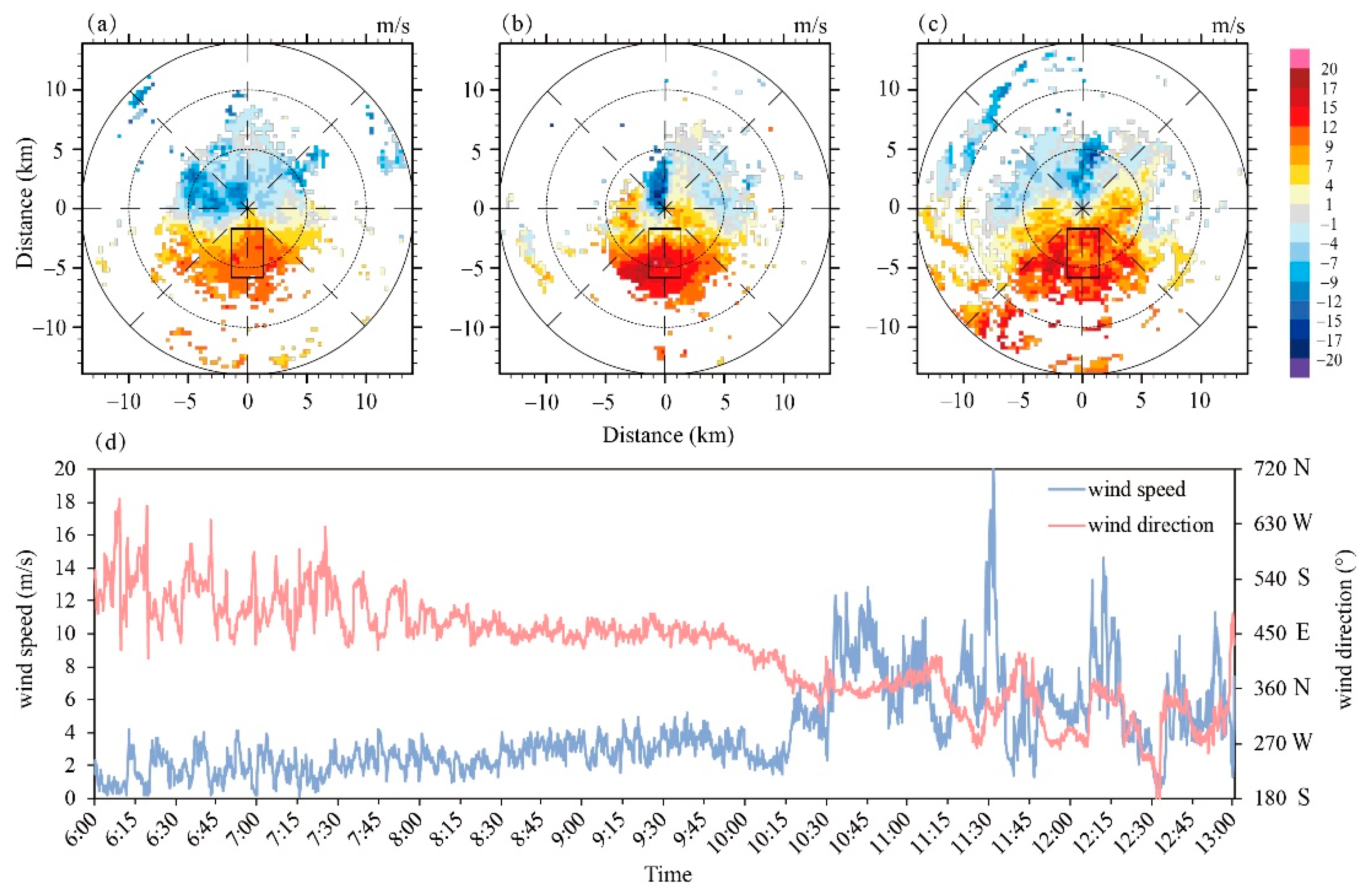
2. Overview of LLW Case

On 15 October 2016, two sequential LLW events were reported at ZLLL by pilots at 11:28 and 11:31 UTC, respectively, which caused flights to discontinue their approach and turn around at 1–2 nautical miles (NM) away from the runway end. As they were very close in terms of the occurrence time, these two LLW events are treated as one LLW process in our work. Based on synoptic analysis using NCEP-FNL data from 12:00 UTC 15 October 2016, there was an upper-level jet at 200 hPa with a maximum wind speed > 48 m/s above ZLLL (Figure 1a), and ZLLL was located behind an eastward shortwave trough at 500 hPa (Figure 1b), with the 588-ridge line of the steady western Pacific subtropical high being maintained at around 25° N. At 700 hPa, a low-level jet existed in the north of Gansu Province at about 42° N, and a large wind speed gradient appeared over ZLLL (Figure 1c). Moreover, ZLLL is in a region with wind changes and a 2 m relative humidity (RH) < 40% (Figure 1d). According to our previous studies, this LLW case is a northerly wind-type LLW, which is a common type that occurs in ZLLL [15].

The Doppler wind lidar that captured the LLW case at ZLLL has a detection range of up to 14 km, with a 200 m radial resolution. More detailed information is provided in Li et al. [15]. As shown in Figure 2b, LLW was located 1–2 NM south of the lidar at 11:27 UTC (square area), where the radial velocity (Vr) exceeded 19 m/s and the difference in Vr reached 13.35 m/s at a 2.4 km distance. Figure 2a,c present the patterns of Vrs with an approximately 10 min interval before (11:18 UTC) and after (11:36 UTC) the occurrence of this LLW. At 11:18 UTC, no wind shear occurred, although the Vr was 9–12 m/s (Figure 2a). After the LLW occurrence, the areas of high velocities were scattered to the south of the lidar (Figure 2c).

The temporal evolution of wind around the timing of LLW (Figure 2d) can be reflected by the AWOS installed at the center of the ZLLL runway, which measured the wind speed and direction at 10 m every 15 s. During 06:00–10:15 UTC, the wind speed was stable and low, with an average speed of 2.4 m/s, and a southeasterly wind prevailed around the runway. After 10:15 UTC, the wind speed increased and fluctuated sharply, when the wind direction turned northerly. At around 11:30 UTC, the wind speed changed drastically in a few minutes, reaching a maximum of 20 m/s. This indicates that LLW happened at a small temporal scale and with high variability.

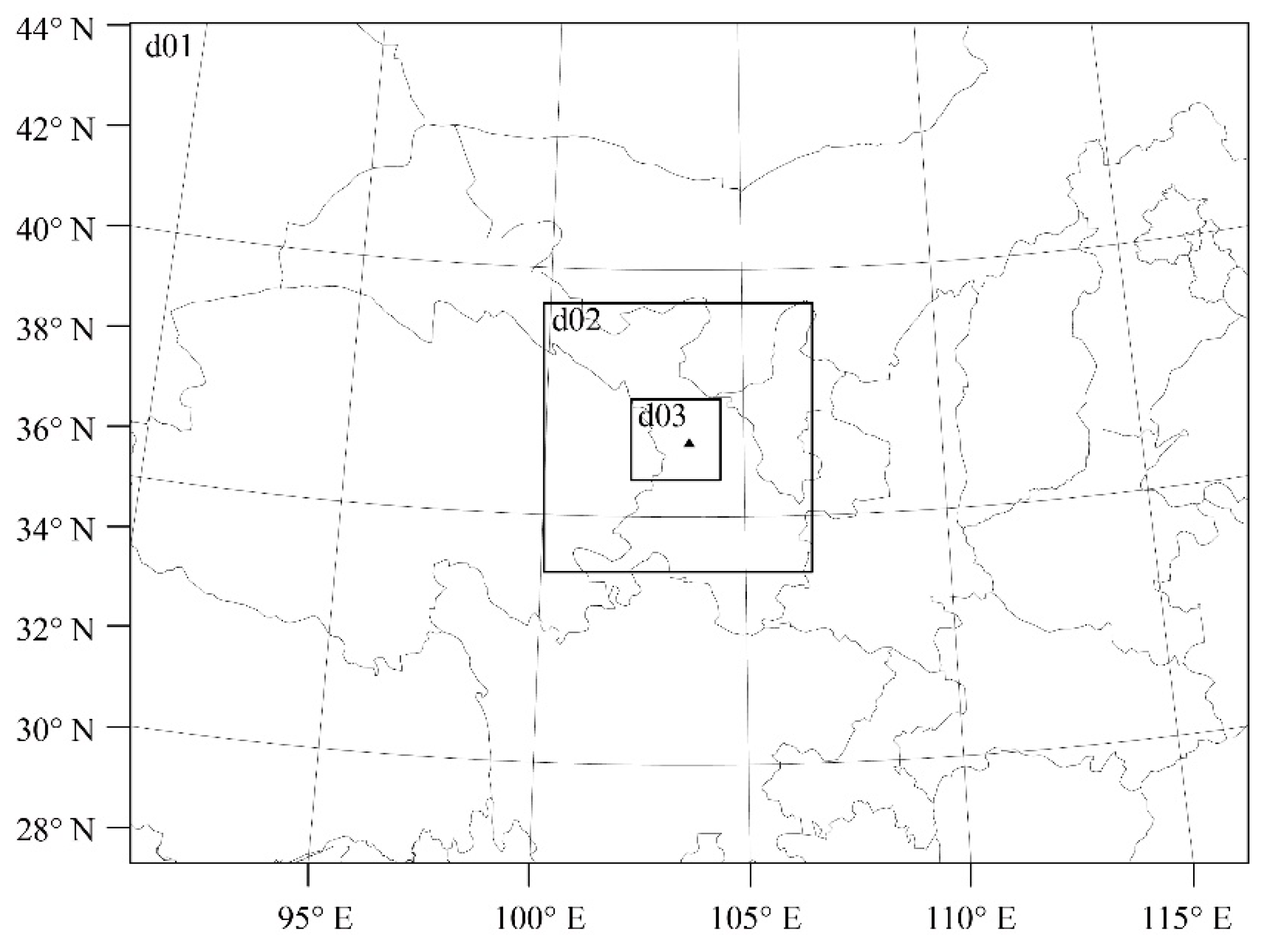
3. Experimental Design

The operational LLW prediction based on the WRF model and its three-dimensional variational (3D-VAR) system at HKIA is promising [3], so in this study, we followed up on the WRF model and its 3DVar system (version 3.8.1) to perform LLW assimilation and simulation experiments. All experiments were configured with three one-way nested domains (Figure 3) centered at 36.51° N, 103.62° E. The spatial resolutions were 25 (D01, 101 × 76), 5 (D02, 121 × 121), and 1 km (D03, 201 × 181). The model top was 50 hPa. The physics schemes used in all domains include the Rapid Radiative Transfer Model longwave radiation [24], Dudhia shortwave radiation [25], the Yonsei University (YSU) planetary boundary layer scheme [26], the Purdue–Lin microphysics scheme [27,28], and the Noah land surface scheme [29]. The Kain–Fritsch convective parameterization scheme [30] was only used for the outer domain D01. Experiments were initialized using the NCEP-FNL global analysis data with 1° × 1° grid points available every 6 h. For the inner domains, the initial and boundary conditions were generated by the model output from the outer domain.

In our original experimental setting, four one-way nested domains were employed, including the above three domains and an innermost domain with a 200 m resolution (D04, 201 × 201). By verifying the simulation results with 1 km and 200 m resolutions against observations from the lidar and AWOS, we found that the simulation with a 200 m resolution performed slightly worse than that with a 1 km resolution. This conclusion is consistent with Boilley and Mahfouf [11], in which the use of a higher horizontal resolution (500 m) in the NWP model did not provide a real improvement in the simulation of the location and time for LLWs associated with synoptic phenomena. Therefore, three one-way nested domains were used in the following assimilation and simulation experiments.

A total of eight experiments were designed (

Table 1. Details of experimental designs.

Count	Experimental Name	Eta Level	Assimilation Setting
			Cycle Interval	Assimilation Timespan
1	CON	30	Without assimilation
2	CONL60	60	Without assimilation
3	DL1h	30	1 h	0700–1100
4	DL30m	30	30 min	0700–1100
5	DL10m	30	10 min	0700–1100
6	DL10mL60	60	10 min	0700–1100
7	DL10mCycle	30	10 min	0700–1300
8	DL10mL60Cycle	60	10 min	0700–1300

), in which different assimilation intervals and timespans were examined to investigate the impact of lidar DA on LLW simulations. In addition, we also tested the influence of the vertical resolution, including 30 (L30) and 60 eta levels (L60), in which the eta coordinate is a terrain-following hydrostatic-pressure vertical coordinate used in the WRF model. L30 came from the default model setting and L60 refers to the setting of the European Centre for Medium Range Weather Forecasts (ECMWF, https://www.ecmwf.int/en/forecasts/documentation-and-support/60-model-levels). As Table 1 shows, experiments CON and CONL60 were performed with the WRF model without DA, in which the suffix “L60” represents the 60 eta level; otherwise, the 30 eta level was used. The simulation period was 06:00–13:00 UTC 15 October 2016. Another six experiments were performed, in which the prefix “DL” indicates that lidar data were assimilated in the innermost domain, and the suffixes “1h”, “30m”, and “10m” denote the different assimilation intervals at 1 h, 30 min, and 10 min, respectively. The first guess for the initial 3D-Var analysis was provided by the 1 h forecast from the WRF model output at 07:00 UTC. Specifically, the background error covariance was estimated using the National Meteorological Center (NMC) method [31] from month-long 24 and 12 h forecasts valid for October 2016. For the two assimilation experiments with the suffix “cycle”, the DA period was 07:00–13:00 UTC, while the other four assimilation experiments (named DL1h, DL30m, DL10m, and DL10mL60) were carried out over 07:00–11:00 UTC.

The Vrs at a three- and six-degree elevation used in the assimilated experiments were first subjected to quality control and outlier removal [15], and then preprocessed to model grid points via the 88d2arps program in the ARPS system [32]. The error of Vr for the assimilation experiments was specified as 1 m/s.

4. Results

4.1. Increment Analysis

To assess the ability of lidar DA to absorb lidar data, the increment fields from assimilation experiments were analyzed by using Vr differences between observations and their model equivalents in both the analysis (O-A: observation minus analysis) and background (O-B: observation minus background).

Figure 4 displays the distributions of O-B and O-A for experiments DL1h, DL30m, DL10m, and DL10mL60 at 07:00 and 10:00 UTC, respectively. With the assimilation of Vrs, the departures between observations and their model equivalents were reduced significantly. The difference can be seen for experiments DL10m and DL10mL60 at the beginning of the assimilation cycle (07:00 UTC) (Figure 4a,b). At this moment, O-B is distributed from −2.5 to 2.5 m/s, while O-A is distributed from −1.5 to 1.5 m/s, with an almost Gaussian curve. Moreover, the numbers of departures among [−0.5, 0.5] increased from 165 (O-B) to 343 (O-A) for the lower vertical resolution (30 eta level) and from 172 (O-B) to 363 (O-A) for the higher resolution L60. This implies that L60 works slightly better than L30 for providing first guess fields. With the assimilation process, experiments with a small assimilation interval (e.g., 10 min) have a better ability to absorb observed data, as shown by the experimental results at 10:00 UTC (Figure 4c,d). The O-B departure is distributed broadly in [–5, 5] m/s, while the O-A value is concentrated at [–2, 2] m/s at 10:00 UTC.

The increase in the vertical resolution also plays a positive role in the assimilation ability (Figure 4). At 07:00/10:00 UTC, there were 83.26%/83.89% O-A departures concentrated at [−0.5, 0.5] in the experiment with L60, while these were 78.67%/77.64% in the DL10m experiment. Additionally, the significant influence of different assimilation intervals can be observed in the results. For example, many observations were rejected in experiments DL1h and DL30m because of the large differences between observations and backgrounds at 10:00 UTC. In other words, about 30% of the data points were assimilated in experiments DL1h and DL30m, whereas nearly 70% of the data points were assimilated in experiments with a 10 min interval.

4.2. Comparison with Lidar Observations

To investigate the impact of lidar DA on LLW simulations, the results from the eight experiments were verified against lidar observations at ZLLL. The estimated lidar data were calculated from modeled three-dimensional wind components (U, V, and W) from the 1 km-resolution model output at the observed location of the Doppler wind lidar. Subsequently, the root mean square error (RMSE) and correlation coefficient (CC) between the observation and their model equivalents were calculated. At 11:00 UTC, 30 min before the LLW occurrence, the spatial distribution of Vrs estimated from the two experiments without DA (CON and CONL60) exhibited obvious differences from lidar observations (RMSE > 7 m/s,

Table 2. Root mean square errors (RMSEs) and correlation coefficients (CCs) between observed Vrs and estimated lidar data from eight experiments.

Time	11:00		11:10		11:20		11:30
Experiments	CC	RMSE	CC	RMSE	CC	RMSE	CC	RMSE
CON	0.603	7.173	0.616	5.878	0.319	7.320	0.334	8.572
CONL60	0.608	7.159	0.601	6.029	0.301	7.507	0.308	8.682
DL1h	0.931	3.535	0.870	3.753	0.465	6.929	0.312	8.939
DL30m	0.932	3.544	0.834	4.121	0.387	8.037	0.274	9.442
DL10m	0.955	2.694	0.790	4.824	0.259	8.568	0.153	9.898
DL10mL60	0.937	3.184	0.737	5.579	0.184	9.206	0.167	9.540
DL10mCycle	0.955	2.694	0.920	2.889	0.855	3.522	0.755	5.021
DL10mL60Cycle	0.937	3.184	0.896	3.314	0.850	3.670	0.638	5.918

), and the magnitude of estimated Vrs was relatively small (Figure 5a,f,i). However, the results from all assimilation experiments were consistent with the observations, including similar distributions and magnitudes (Figure 5b–e,g,h). The RMSEs were decreased by half or more, while the CCs were increased to >0.93 compared to experiments without DA (Table 2). Moreover, assimilation experimental results with 10 min assimilation intervals showed a greater consistency with the lidar observation than the results of other experiments (Table 2; Figure 5d,e,g,h). Therefore, lidar DA with a shorter interval is beneficial for simulating the wind field, which can absorb more observed information, as shown in the O-A analysis in Section 4.1. Furthermore, similar results were found in experiments with a different vertical resolution, but the DA experiment with L30 performed slightly better than that with L60 (as shown by RMSE and CC in Table 2). This may be reflected in certain details, such as the fact that the weak negative value obtained from experiment DL10m became a weak positive value in experiment DL10mL60 to the northwest of the lidar.

Since wind shear occurred at 11:28 and 11:31 UTC, we further verified the experimental results from the eight experiments against lidar observations at 11:30 UTC. The observations showed that the velocity difference was >7.7 m/s to the south side of the lidar (Figure 6i) when LLW occurred. Lidar Vrs calculated from all experiments displayed obvious differences (Table 2; Figure 6). The Vrs from the two experiments without DA (CON and CONL60) had similar spatial distributions and there were large differences (RMSE > 8 m/s) from observations (Table 2; Figure 6a,f). Among all DA experiments, only DL10mCycle and DL10mL60Cycle had similar distributions to lidar observations with smaller RMSEs, while others exhibited more consistency with experiments without DA (Table 2; Figure 6b–d,g). From these experiments that ended the assimilation cycle at 11:00 UTC, the lidar assimilation had an obvious positive effect in estimating wind fields at 11:00 UTC. However, this effect declined with an increasing integration time. At 11:30 UTC, the assimilation experiments did not perform well, and even worse than the CON experiment without DA, which can be seen from the RMSEs and CCs in Table 2. Though the DL1h experiment worked better than the DL30m and DL10m experiments at 11:30 UTC, the experimental result is almost close to the results from the CON experiment (Table 2). This means that the role of lidar DA was mainly maintained in the first 10–20 min after the assimilation time. The cycling experiments (DL10mCycle and DL10mCycleL60) ended at 13:00 UTC reproduced similar characteristics for the Vr to lidar observations at 11:30 UTC (Figure 6e,h), whose RMSEs are smaller than other experimental results (Table 2). In this case, a smaller assimilation interval is required for LLW simulation. However, the Vr magnitude obtained with 30 eta levels (experiment DL10mCycle) was closer to the lidar observations than DL10mCycleL60 (Figure 6e,h), and DL10mCycle obtained a smaller RMSE and higher CC (Table 2).

4.3. Comparison with AWOS Observation

Another available observation was obtained from the AWOS installed at ZLLL. The U and V components at 10 m were calculated from the 1 km-resolution model output and used for the comparison with the AWOS observation. Figure 7 presents the time evolutions of the observed wind information and their model equivalents from eight experiments, and

Table 3. RMSEs and CCs of observed 10 m U and V components and their model equivalents from eight experiments.

Experiment Name	U Component (m/s)		V Component (m/s)
	CC	RMSE	CC	RMSE
CON	−0.493	4.185	0.495	2.966
CONL60	−0.258	4.116	0.508	2.924
DL1h	−0.298	4.284	0.502	2.994
DL30m	−0.358	4.490	0.604	2.706
DL10m	−0.277	4.483	0.741	2.265
DL10mL60	−0.085	3.979	0.751	2.228
DL10mCycle	0.489	3.134	0.803	2.055
DL10mL60Cycle	0.508	3.012	0.804	2.030

lists the RMSEs and CCs between their observations and simulations.

Identical to the description in Section 2, a weak wind can be observed for 06:00–10:15 UTC, which then changed rapidly after 10:15 UTC (Figure 7). All experiments have a good ability to simulate the wind field during 06:00–10:15 UTC, while there are obvious differences from different experiments after 10:15 UTC. Experiments CON and CONL60 have no ability to simulate LLW because the features of LLW with a rapid change of wind are not found throughout the entire simulation period (Figure 7). In contrast, DA experiments can obtain the wind change after 10:15 UTC, but there is a difference when using different assimilation intervals in the assimilation experiments. U and V components estimated from experiments with a large assimilation interval deviate from the analysis quickly and lead to a large RMSE (e.g., the green dashed line in Figure 7; Table 3), while experiments with a smaller interval perform better at maintaining the trend of wind (e.g., the green solid line in Figure 7). As mentioned in Section 4.2, the role of DA is only maintained for about 10–20 min, which results in a difference between experiments with different assimilation timespans (e.g., experiments DL10m and DL10mCycle). Experiment DL10mL60Cycle performed slightly better than DL10mCycle (Table 3), which indicates that the 60 eta level has a positive role in simulating wind fields at a lower altitude. In addition, the simulation accuracy of V components is higher than that of U components (Table 3), which could be because the assimilated Vrs along the runway are consistent with the direction of V components.

4.4. Model-Based Analysis

In this section, the better simulation results from experiment DL10mL60Cycle are used for further analysis. Figure 8 displays the cross-sections of the wind field, vertical velocity, and pseudo-equivalent potential temperature θse. In the latitude cross-section, high wind speeds reaching up to 11.8 m/s are concentrated at a distance of 2–3 km, where LLW occurred (1–2 NM south of ZLLL, Figure 8a), which is a good representation of the small-scale characteristics of LLW. A large wind gradient can be found south of the maximum wind speed, with a variance of 11.8–1.5 m/s within 7 km (Figure 8a). In particular, a significant downdraft flow, along with a high wind speed, mainly covered the upper area of ZLLL (Figure 8d,e). In addition, as θse decreased with height at <500 hPa (Figure 8d,e), updrafts (Figure 8b,c,e) accompanied by a higher RH (Figure 8a,b) appeared at the west and north sides of ZLLL, which indicates that the atmosphere at ZLLL was unstable and conducive to the development of convection. All of these conditions are favorable for the LLW process. Therefore, flights landing at ZLLL from south to north would first go through an increasing headwind (headwind shear) and then decreasing headwind (tailwind shear), accompanied by a downdraft (Figure 8a).

The above simulation results are consistent with the LLW information provided by wind lidar observations. The results also indicate that the LLW has a small temporal and spatial scale. In this case, accurately predicting LLW is not a straightforward matter, as any small change in the initial field may create a different simulation result. As shown in Section 4.2 and Section 4.3, experiments without DA and with an assimilation cycle that ended at 11:00 UTC displayed a limitation in simulating LLW.

5. Conclusions

LLW occurs with rapid changes in the wind direction or speed, whose small-scale and short-lived characteristics make its accurate simulation and prediction difficult. Doppler wind lidar, as an effective tool for detecting LLW, has not been used efficiently in the numerical simulation of LLW. In this study, we aim to assimilate high temporal–spatial Doppler wind lidar observations into the NWP model to improve the simulation ability of LLW and examine the impact of lidar DA through different assimilation intervals and vertical resolutions. The following conclusions can be drawn:

• Experiments without DA have no ability to capture the small-scale features of LLW at ZLLL. The lidar DA can effectively absorb lidar observations, and consequently improve the simulation ability of the WRF model on LLW;
• Assimilation experiments with a small interval (e.g., 10 min) are beneficial for the simulation of LLW, whereas experiments with a large interval are unfavorable for maintaining the development of the wind field. Moreover, a higher vertical resolution (L60) may not provide much improvement in simulating LLW at ZLLL;
• The simulation results indicate that this LLW case occurred at a small temporal and spatial scale, accompanied by a large wind speed gradient in the southern area of ZLLL. A small change in the initial field may result in different simulation results;
• The accurate simulation of LLW is helpful for improving aviation safety. Since LLW can occur in various weather conditions, more LLW case studies and experiments should be conducted in the future for the application of lidar DA in LLW simulation and prediction.

References

1. International Civil Aviation Organization (ICAO). Meteorological Service for International Air Navigation: Annex 3 to the Convention on International Civil Aviation, 16th ed.; ICAO: Montréal, QC, Canada, 2007; p. 187. [Google Scholar]
2. Nechaj, P.; Gaál, L.; Bartok, J.; Vorobyeva, O.; Gera, M.; Kelemen, M.; Polishchuk, V. Monitoring of Low-Level Wind Shear by Ground-based 3D Lidar for Increased Flight Safety, Protection of Human Lives and Health. Int. J. Environ. Res. Public Health 2019, 16, 4584. [Google Scholar] [CrossRef] [PubMed] [Green Version]
3. Hon, K.-K. Predicting Low-Level Wind Shear Using 200-m-Resolution NWP at the Hong Kong International Airport. J. Appl. Meteorol. Clim. 2020, 59, 193–206. [Google Scholar] [CrossRef]
4. Fujita, T.T.; Caracena, F. An Analysis of Three Weather-Related Aircraft Accidents. Bull. Am. Meteorol. Soc. 1977, 58, 1164–1181. [Google Scholar] [CrossRef]
5. International Civil Aviation Organization (ICAO). Manual on Low-Level Wind Shear and Turbulence; ICAO: Montréal, QC, Canada, 2005; p. 222. [Google Scholar]
6. Benjamin, S.G.; Brown, J.M.; Brunet, G.; Lynch, P.; Saito, K.; Schlatter, T.W. 100 Years of Progress in Forecasting and NWP Applications. Meteorol. Monogr. 2019, 59, 13.1–13.67. [Google Scholar] [CrossRef]
7. Clark, T.L.; Keller, T.; Coen, J.; Neilley, P.; Hsu, H.-M.; Hall, W.D. Terrain-Induced Turbulence over Lantau Island: 7 June 1994 Tropical Storm Russ Case Study. J. Atmos. Sci. 1997, 54, 1795–1814. [Google Scholar] [CrossRef] [Green Version]
8. Cheung, J.O.P.; Chan, P.W.; Leung, D.Y.C. Large-eddy simulation of the wind flow across a terminal building on the airfield. Int. J. Earth Sci. Eng. 2011, 4, 486–489. [Google Scholar]
9. Li, L.; Chan, P.W.; Zhang, L.; Hu, F. Numerical Simulation of a Lee Wave Case over Three-Dimensional Mountainous Terrain under Strong Wind Condition. Adv. Meteorol. 2013, 2013, 1–13. [Google Scholar] [CrossRef]
10. Carruthers, D.; Ellis, A.; Hunt, J.; Chan, P.W. Modelling of wind shear downwind of mountain ridges at Hong Kong International Airport. Meteorol. Appl. 2014, 21, 94–104. [Google Scholar] [CrossRef] [Green Version]
11. Boilley, A.; Mahfouf, J.-F. Wind shear over the Nice Côte d’Azur airport: Case studies. Nat. Hazards Earth Syst. Sci. 2013, 13, 2223–2238. [Google Scholar] [CrossRef] [Green Version]
12. Jiang, L.H.; Qin, Y.T.; Yang, Y.Y.; Wang, Z. Microscale Numerical Simulation about Field Wind and Wind Shear with the Aviation Numerical Weather Prediction Model. Sci. Tech. Eng. 2016, 16, 156–161. (In Chinese) [Google Scholar] [CrossRef]
13. Chan, P.W.; Hon, K.K. Performance of super high resolution numerical weather prediction model in forecasting terrain-disrupted airflow at the Hong Kong International Airport: Case studies. Meteorol. Appl. 2016, 23, 101–114. [Google Scholar] [CrossRef]
14. Shun, C.M.; Chan, P.W. Applications of an Infrared Doppler Lidar in Detection of Wind Shear. J. Atmos. Ocean. Technol. 2008, 25, 637–655. [Google Scholar] [CrossRef]
15. Li, L.; Shao, A.; Zhang, K.; Ding, N.; Chan, P.-W. Low-Level Wind Shear Characteristics and Lidar-Based Alerting at Lanzhou Zhongchuan International Airport, China. J. Meteorol. Res. 2020, 34, 633–645. [Google Scholar] [CrossRef]
16. Keohan, C.F.; Barr, K.; Hannon, S.M. Evaluation of Pulsed Lidar Wind Hazard Detection at Las Vegas International Airport. In Proceedings of the 12th Conference on Aviation, Range, and Aerospace Meteorology, Atlanta, GA, USA, 29 January–2 February 2006. [Google Scholar]
17. Matayoshi, N.; Iijima, T.; Yamamoto, K.; Fujita, E. Development of Airport Low-level Wind Information (ALWIN). In Proceedings of the 16th AIAA Aviation Technology, Integration, and Operations Conference, Washington, DC, USA, 13–17 June 2016. [Google Scholar]
18. Chen, Y.; An, J.; Wang, X.; Sun, Y.; Wang, Z.; Duan, J. Observation of wind shear during evening transition and an estimation of submicron aerosol concentrations in Beijing using a Doppler wind lidar. J. Meteorol. Res. 2017, 31, 350–362. [Google Scholar] [CrossRef]
19. Zhang, H.; Wu, S.; Wang, Q.; Liu, B.; Yin, B.; Zhai, X. Airport low-level wind shear lidar observation at Beijing Capital International Airport. Infrared Phys. Technol. 2019, 96, 113–122. [Google Scholar] [CrossRef] [Green Version]
20. Thobois, L.; Cariou, J.P.; Gultepe, I. Review of Lidar-Based Applications for Aviation Weather. Pure Appl. Geophys. 2019, 176, 1959–1976. [Google Scholar] [CrossRef]
21. Choy, B.L.; Lee, O.S.M.; Shun, C.M.; Cheng, C.M. Prototype Automatic LIDAR- Based Wind Shear Detection Algorithms. In Proceedings of the 11th Conference on Aviation, Range, and Aerospace Meteorology, Hyannis, MA, USA, 3–8 October 2004. [Google Scholar]
22. Tang, W.; Chan, P.W.; Haller, G. Lagrangian Coherent Structure Analysis of Terminal Winds Detected by Lidar. Part I: Turbulence Structures. J. Appl. Meteorol. Clim. 2011, 50, 325–338. [Google Scholar] [CrossRef] [Green Version]
23. Kawabata, T.; Iwai, H.; Seko, H.; Shoji, Y.; Saito, K.; Ishii, S.; Mizutani, K. Cloud-Resolving 4D-Var Assimilation of Doppler Wind Lidar Data on a Meso-Gamma-Scale Convective System. Mon. Weather Rev. 2014, 142, 4484–4498. [Google Scholar] [CrossRef]
24. Mlawer, E.J.; Taubman, S.J.; Brown, P.D.; Iacono, M.J.; Clough, S.A. Radiative transfer for inhomogeneous atmospheres: RRTM, a validated correlated-k model for the longwave. J. Geophys. Res. Space Phys. 1997, 102, 16663–16682. [Google Scholar] [CrossRef] [Green Version]
25. Dudhia, J. Numerical study of convection observed during the winter monsoon experiment using a mesoscale two dimensional model. J. Atmos. Sci. 1989, 46, 3077–3107. [Google Scholar] [CrossRef]
26. Hong, S.-Y.; Noh, Y.; Dudhia, J. A New Vertical Diffusion Package with an Explicit Treatment of Entrainment Processes. Mon. Weather Rev. 2006, 134, 2318–2341. [Google Scholar] [CrossRef] [Green Version]
27. Lin, Y.-L.; Farley, R.D.; Orville, H.D. Bulk Parameterization of the Snow Field in a Cloud Model. J. Clim. Appl. Meteorol. 1983, 22, 1065–1092. [Google Scholar] [CrossRef] [Green Version]
28. Chen, S.-H.; Sun, W.-Y. A One-dimensional Time Dependent Cloud Model. J. Meteorol. Soc. Jpn. 2002, 80, 99–118. [Google Scholar] [CrossRef] [Green Version]
29. Chen, F.; Dudhia, J. Coupling an advanced land surface-hydrology model with the Penn State-NCAR MM5 modeling system. Part I: Model implementation and sensitivity. Mon. Weather Rev. 2001, 129, 569–585. [Google Scholar] [CrossRef] [Green Version]
30. Kain, J.S. The Kain–Fritsch Convective Parameterization: An Update. J. Appl. Meteor. 2004, 43, 170–181. [Google Scholar] [CrossRef] [Green Version]
31. Parrish, D.F.; Derber, J.C. The National Meteorological Center’s Spectral Statistical-Interpolation Analysis System. Mon. Weather Rev. 1992, 120, 1747–1763. [Google Scholar] [CrossRef]
32. Brewster, K.; Hu, M.; Xue, M.; Gao, J. Efficient Assimilation of Radar Data at High Resolution for Short-Range Numerical Weather Prediction. In Proceedings of the World Weather Research Program Symposium on Nowcasting and Very Short-Range Forecasting, WSN05, Tolouse, France, 5–9 September 2005. [Google Scholar]
Figure 1. Horizontal distributions of the geopotential height (contour; dagpm) and wind vectors (m s–1) at (a) 200, (b) 500, and (c) 700 hPa, and (d) 2 m relative humidity (RH) (filled; %) and 10 m wind vectors from the NCEP final (FNL) data at 12:00 UTC on 15 October 2016. The filled areas in (a,c) indicate the upper-level jet and low-level jet with a wind speed > 40 and > 12 m/s, respectively. The thick black lines represent troughs, and the red triangle indicates the site of Lanzhou Zhongchuan International Airport (ZLLL).
Atmosphere 11 01342 g001
Figure 2. Lidar plan position indicator (PPI) scan for Vrs at a six-degree elevation at (a) 11:18 UTC, (b) 11:27 UTC, and (c) 11:36 UTC, respectively, and (d) time series of the 10 m wind speed (blue) and wind direction (red) observed by an automated weather observing system (AWOS).
Atmosphere 11 01342 g002
Figure 3. The model domains and site of the Doppler lidar (denoted by the triangle).
Atmosphere 11 01342 g003
Figure 4. Background (a,c) and analysis (b,d) departures for lidar radial velocity (Vr) from assimilation experiments at (a,b) 07:00 UTC and (c,d) 10:00 UTC 15 October 2016.
Atmosphere 11 01342 g004
Figure 5. Vrs estimated from experiments (a) CON, (b) DL1h, (c) DL30m, (d) DL10m, (e) DL10mCycle, (f) CONL60, (g) DL10mL60, and (h) DL10mL60Cycle, and (i) observations at a six-degree elevation at 11:00 UTC.
Atmosphere 11 01342 g005
Figure 6. Vrs estimated from experiments (a) CON, (b) DL1h, (c) DL30m, (d) DL10m, (e) DL10mCycle, (f) CONL60, (g) DL10mL60, and (h) DL10mL60Cycle, and (i) observations at a six-degree elevation at 11:30 UTC.
Atmosphere 11 01342 g006
Figure 7. Time series of 10 m (a) U and (b) V components observed by the AWOS station and their model equivalents from eight experiments. The shaded areas indicate the maximum and minimum observations in 10 min.
Atmosphere 11 01342 g007
Figure 8. Latitude (a) and longitude (b) pressure cross-sections of the wind vector and speed (white line; m/s), RH (shaded; %). Horizontal distribution of vertical velocity (c) at 700 hPa. Latitude (d) and longitude (e) pressure cross-sections of the vertical velocity (shaded; m/s) and pseudo-equivalent potential temperature θse (contour; K) at 11:30 UTC from the experiment DL10mL60Cycle. The five-pointed star indicates the site of ZLLL and the vertical velocities are magnified five-fold to visualize the vertical motion.
Atmosphere 11 01342 g008