Modeling Maximum Tsunami Heights Using Bayesian Neural Networks


Abstract
:1. Introduction
2. Numerical Simulation
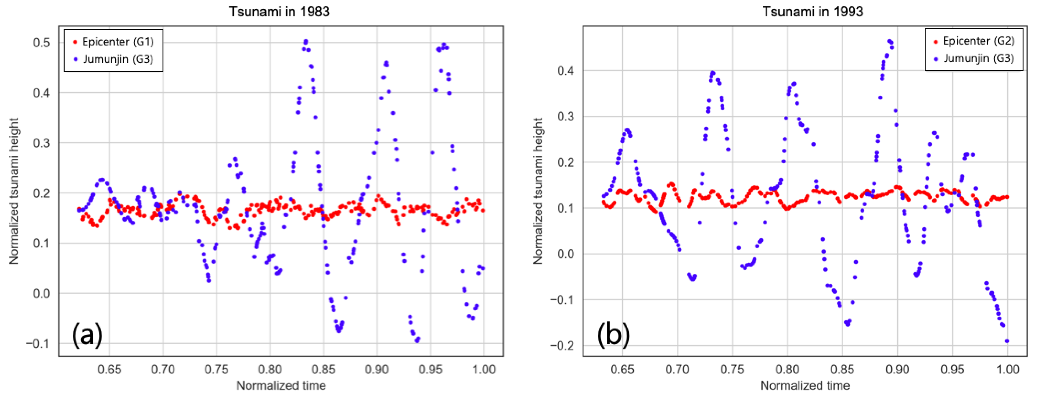
2.1. Propagation
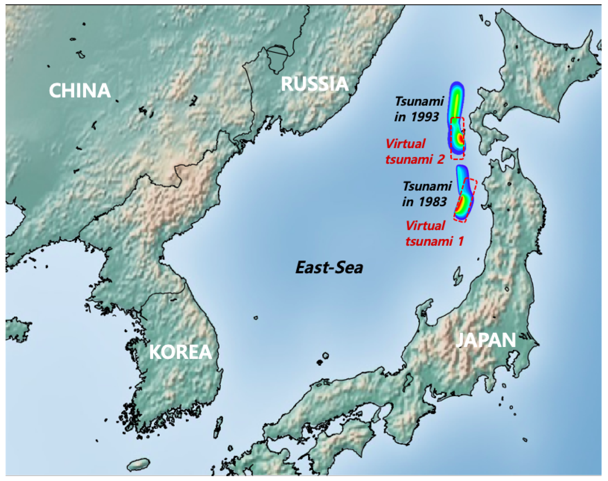
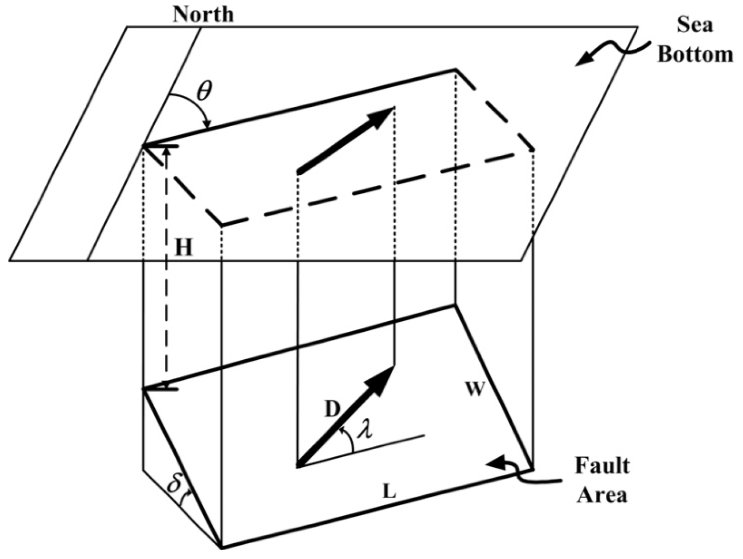
2.2. Initial Free Surface Displacement
3. Bayesian Neural Networks
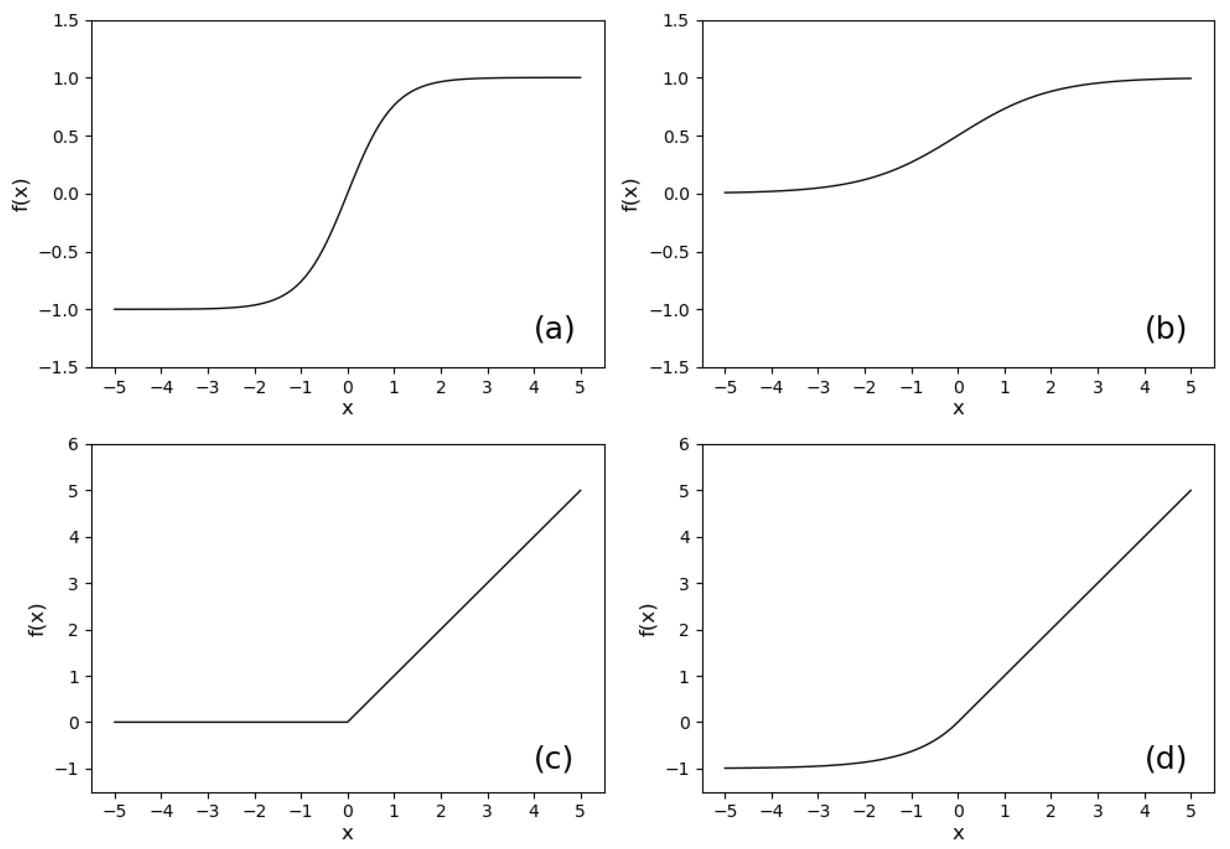
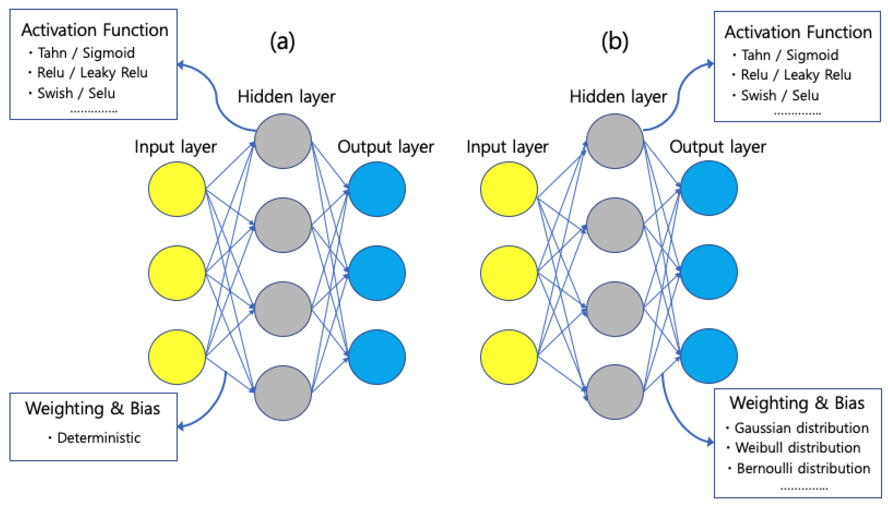
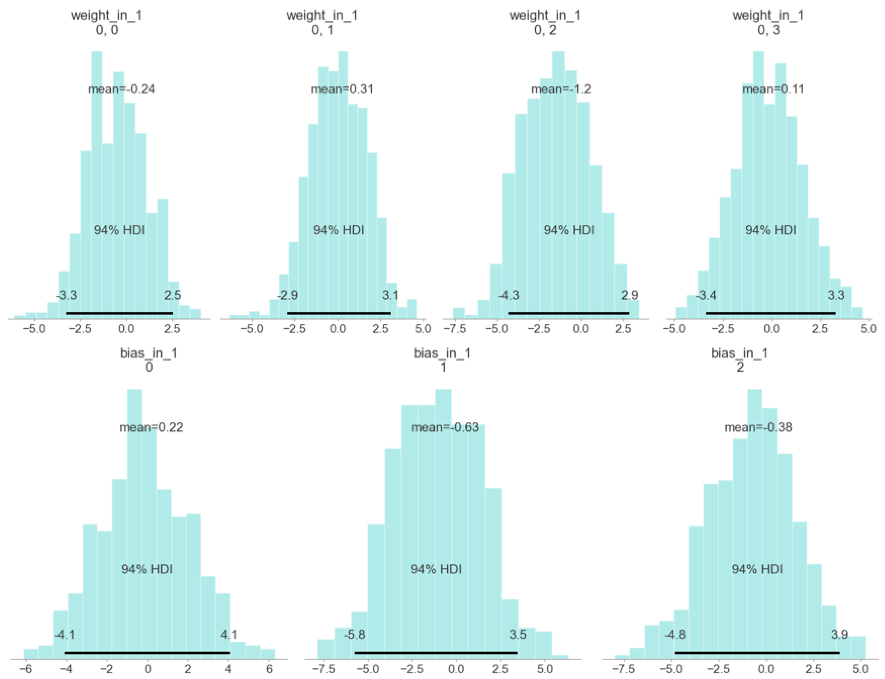
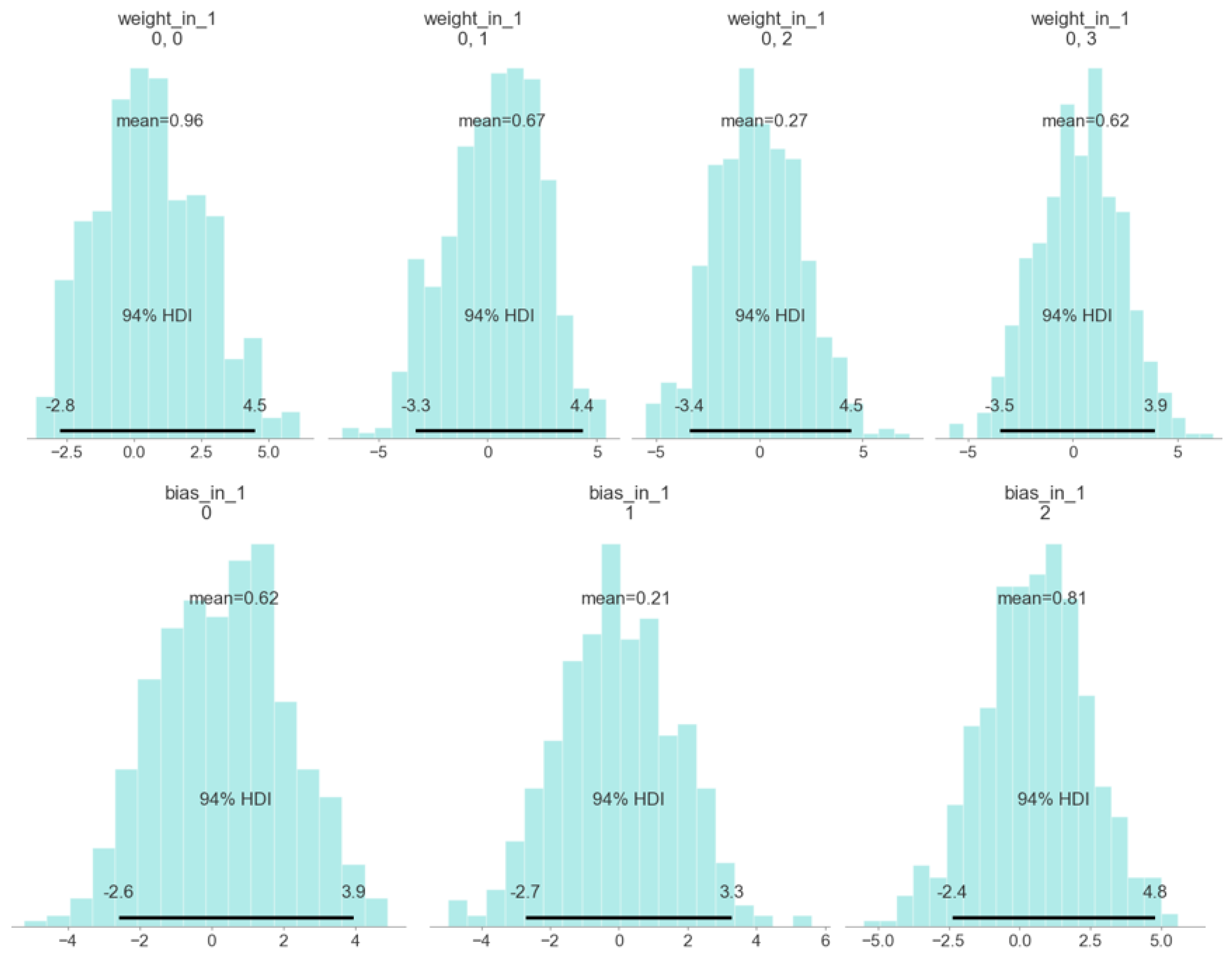
3.1. Neural Networks
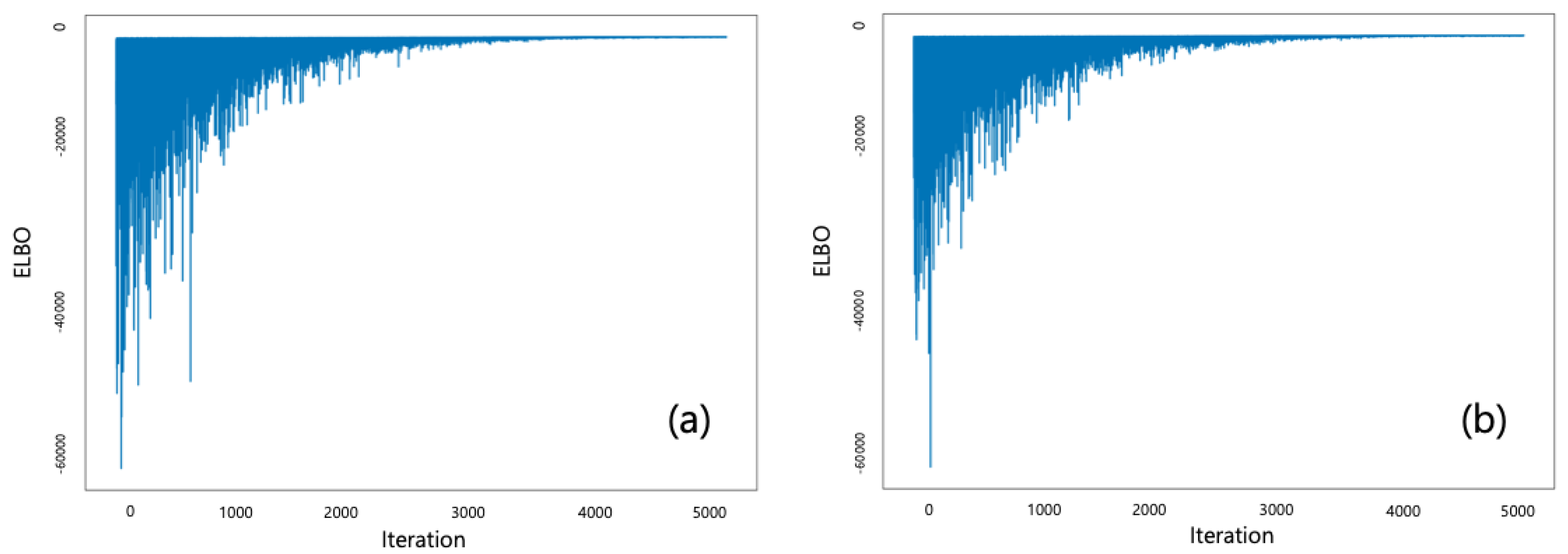
3.2. Bayesian Inference
4. Results
4.1. Training
4.2. Testing
4.3. Prediction
5. Summary and Conclusions
Author Contributions
Funding
Acknowledgments
Conflicts of Interest
References
- Cho, Y.-S.; Hwang, H.-S.; Kim, J.-Y.; Kwan, H.-K. Development of Hazard Map with probable maximum tsunamis. J. Coast. Res. 2016, 75, 1057–1061. [Google Scholar] [CrossRef]
- Imamura, F.; Shuto, N.; Goto, C. Numerical simulations of the transoceanic propagation of tsunamis. In Proceedings of the Congress Asian and Pacific Regional Division, Yogyakarta, Indonesia, 8–10 September 1998; pp. 265–272. [Google Scholar]
- Cho, Y.-S.; Liu, P.L.-F. Crest length effects in nearshore tsunami run-up around islands. J. Geophys. Res. 1999, 104, 7907–7913. [Google Scholar] [CrossRef]
- Yoon, S.B. Propagation of tsunamis over slowly varying topography. J. Geophys. Res. 2002, 107, 4-1–4-11. [Google Scholar] [CrossRef]
- Choi, B.H.; Pelinovsky, E.; Hong, S.J.; Woo, S.B. Computation of tsunamis in the East (Japan) Sea using dynamically interfaced nested model. Pure Appl. Geophys. 2003, 160, 1383–1414. [Google Scholar] [CrossRef]
- Cho, Y.-S.; Sohn, D.-H.; Lee, S.-O. Practical modified scheme of linear shallow-water equations for distant propagation of tsunamis. Ocean. Eng. 2007, 34, 1769–1777. [Google Scholar] [CrossRef]
- Hideki, A. Outline of deep learning. In Deep Learning; Muneki, Y., Shinitsi, M., Daisuke, O., Takayuki, O., Bollegala, D.K., Eds.; Kindaikakagusha: Tokyo, Japan, 2015; pp. 9–13. [Google Scholar]
- Itamar, R.; Dalya, B.; Sahar, S. Probabilistic Random Forest: A Machine Learning Algorithm for Noisy Data sets. Astron. J. 2019, 157, 1–12. [Google Scholar]
- Zoubin, G. Probabilistic machine learning and artificial intelligence. Nature 2015, 521, 452–459. [Google Scholar]
- Suyama, A. Machine learning and bayesian learning. In Introduction to Machine Learning by Bayesian Inference; Sugiyama, M., Ed.; Kodansha: Tokyo, Japan, 2017; pp. 82–85, 121–123. [Google Scholar]
- Back, U.-S. 1983 Tsunami in East-Sea; Korea Meteorology Administration: Seoul, Korea, 1983; p. 44. [Google Scholar]
- Korean Peninsula Energy Development Organization. Estimation of Tsunami Height for KEDO LWR ProjecT Report; Korea Power Engineering Company: Seoul, Korea, 1999. [Google Scholar]
- Kim, K.-H.; Cho, Y.-S.; Kwon, H.-H. An integrated Bayesian approach to the probabilistic tsunami risk model for the location and magnitude of earthquakes: Application to the Eastern Coast of the Korean Peninsula. Stoch. Environ. Res. Risk Assess. 2018, 32, 1243–1257. [Google Scholar] [CrossRef]
- Cho, Y.-S. Numerical Simulation of Tsunami Propagation and Run-Up. Ph.D. Dissertation, University of Cornell, NewYork, NY, USA, 1995; pp. 11–52. [Google Scholar]
- Shinichi, N. Probability and bayesian theorem. In Variational Bayesian Learning; Kodansya: Tokyo, Japan, 2019; pp. 79–80. [Google Scholar]
- ASCE Committee. Aritifical Neural Networks in Hydrology: Preliminary concepts. J. Hydrol. Eng. 2000, 5, 115–123. [Google Scholar] [CrossRef]
- Tsoukalas, L.H. Fuzzy Methods in Neural Networks. In Fuzzy and Neural Approaches in Engineering; Uhrig, R.E., Ed.; Wiley: Hoboken, NJ, USA, 1997; pp. 32–58. [Google Scholar]
- Yarin, G. Uncertainty in Deep Learning. Ph.D. Dissertation, University of Cambridge, Cambridge, UK, 2016; pp. 17–20. [Google Scholar]
- Song, M.-J.; Cho, Y.-S. Probabilistic Tsunami Heights Model using Bayesian Machine Learning. J. Coast. Res. 2020, 95, 1291–1296. [Google Scholar] [CrossRef]
- Koki, S. Neural networks. In Deep Learning from Scratch; O’Reilly Japan: Tokyo, Japan, 2016; p. 77. [Google Scholar]
- Afshin, G.; Vladik, K.; Olga, K. Why 70/30 or 80/20 Relation Between Training and Testing Sets: A Pedagogical Explanation; Technical Reports; University of Texas: El Paso, TX, USA, 2018; pp. 1–6. [Google Scholar]
- Amazon Machine Learning: Developer Guide; Amazon: Seattle, WA, USA, 2020; p. 12.


| Classification | Longitude | Latitude | H | L | W | D | M | |||
|---|---|---|---|---|---|---|---|---|---|---|
| (°E) | (°N) | (km) | (°) | (°) | (°) | (km) | (km) | (km) | ||
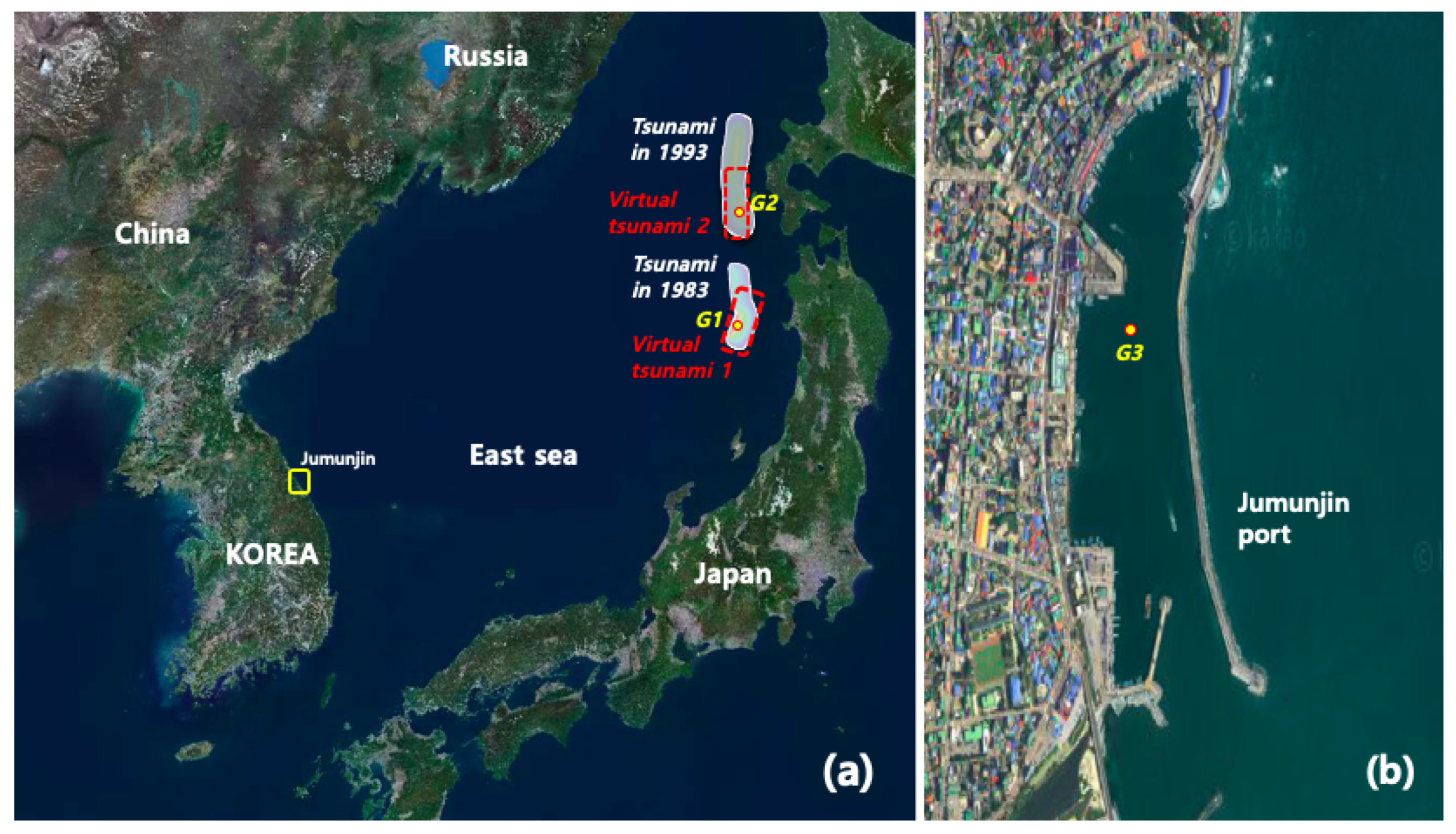
| Tsunami in 1983 | 139.02 | 40.54 | 3 | 355 | 25 | 80 | 60 | 30 | 3.05 | 7.7 |
| 139.30 | 42.10 | 5 | 163 | 60 | 105 | 24.5 | 25 | 12.0 | ||
| Tsunami in 1993 | 139.25 | 42.34 | 5 | 175 | 60 | 105 | 30 | 25 | 2.50 | 7.8 |
| 139.40 | 43.13 | 10 | 188 | 35 | 80 | 90 | 25 | 5.71 | ||
| Virtual tsunami 1 | 138.70 | 40.20 | 1 | 10.0 | 40 | 90 | 125.9 | 62.9 | 6.31 | 8.0 |
| Virtual tsunami 2 | 138.90 | 40.90 | 1 | 5 | 40 | 90 | 125.9 | 62.9 | 6.31 | 8.0 |
| Location | Historical Tsunamis | Numerical Model | BNNs | BIAS (m) | ||
|---|---|---|---|---|---|---|
| Tsunami Height (m) | Tsunami Height (m) | |||||
| Jumunjin | 1983 | 2.26 | 0.0 | 2.9 | 2.31 | +0.05 |
| 1993 | 1.86 | 0.2 | 2.5 | 1.86 | 0.00 | |
| 1.86 | 0.3 | 2.5 | 1.90 | +0.04 | ||
| Location | Virtual Tsunamis | Numerical Model | BNNs | Difference (m) | ||
|---|---|---|---|---|---|---|
| Tsunami Height (m) | Tsunami Height (m) | |||||
| Jumunjin | Virtual tsunami 1 | 2.21 | 0.0 | 2.9 | 2.14 | −0.07 |
| Virtual tsunami 2 | 1.63 | 0.2 | 2.5 | 1.05 | −0.57 | |
| 1.63 | 0.3 | 2.5 | 1.54 | −0.08 | ||
Publisher’s Note: MDPI stays neutral with regard to jurisdictional claims in published maps and institutional affiliations. |
© 2020 by the authors. Licensee MDPI, Basel, Switzerland. This article is an open access article distributed under the terms and conditions of the Creative Commons Attribution (CC BY) license (http://creativecommons.org/licenses/by/4.0/).
Share and Cite
Song, M.-J.; Cho, Y.-S. Modeling Maximum Tsunami Heights Using Bayesian Neural Networks. Atmosphere 2020, 11, 1266. https://doi.org/10.3390/atmos11111266
Song M-J, Cho Y-S. Modeling Maximum Tsunami Heights Using Bayesian Neural Networks. Atmosphere. 2020; 11(11):1266. https://doi.org/10.3390/atmos11111266
Chicago/Turabian StyleSong, Min-Jong, and Yong-Sik Cho. 2020. "Modeling Maximum Tsunami Heights Using Bayesian Neural Networks" Atmosphere 11, no. 11: 1266. https://doi.org/10.3390/atmos11111266