Extending Limited In Situ Mountain Weather Observations to the Baseline Climate: A True Verification Case Study

Abstract

The availability of in situ atmospheric observations decreases with elevation and topographic complexity. Data sets based on numerical atmospheric modeling, such as reanalysis data sets, represent an alternative source of information, but they often suffer from inaccuracies, e.g., due to insufficient spatial resolution. sDoG (statistical Downscaling for Glacierized mountain environments) is a reanalysis data postprocessing tool designed to extend short-term weather station data from high mountain sites to the baseline climate. In this study, sDoG is applied to ERA-Interim predictors to produce a retrospective forecast of daily air temperature at the Vernagtbach climate monitoring site (2640 MSL) in the Central European Alps. First, sDoG is trained and cross-validated using observations from 2002 to 2012 (cross-validation period). Then, the sDoG retrospective forecast and its cross-validation-based uncertainty estimates are evaluated for the period 1979–2001 (hereafter referred to as the true evaluation period). We demonstrate the ability of sDoG to model air temperature in the true evaluation period for different temporal scales: day-to-day variations, year-to-year and season-to-season variations, and the 23-year mean seasonal cycle. sDoG adds significant value over a selection of reference data sets available for the site at different spatial resolutions, including state-of-the-art global and regional reanalysis data sets, output by a regional climate model, and an observation-based gridded product. However, we identify limitations of sDoG in modeling summer air temperature variations particularly evident in the first part of the true evaluation period. This is most probably related to changes of the microclimate around the Vernagtbach climate monitoring site that violate the stationarity assumption underlying sDoG. When comparing the performance of the considered reference data sets, we cannot demonstrate added value of the higher resolution data sets over the data sets with lower spatial resolution. For example, the global reanalyses ERA5 (31 km resolution) and ERA-Interim (80 km resolution) both clearly outperform the higher resolution data sets ERA5-Land (9 km resolution), UERRA HARMONIE (11 km resolution), and UERRA MESCAN-SURFEX (5.5 km resolution). Performance differences among ERA5 and ERA-Interim, by contrast, are comparably small. Our study highlights the importance of station-scale uncertainty assessments of atmospheric numerical model output and downscaling products for high mountain areas both for data users and model developers.

1. Introduction

Availability and quality of in situ meteorological observations dramatically decrease with elevation and topographic complexity (e.g., [1,2,3]). Maintenance of weather stations at high altitudes in complex topography is hampered by many practical obstacles. Most sites are not accessible by car and can be reached only by foot, skis or helicopters; often, the expertise of mountain guides is needed. As a consequence, the stations usually cannot be visited on a daily basis. Furthermore, weather conditions such as strong wind, precipitation as snow, strong precipitation and lightning pose challenges for the design of stations at high altitudes in complex topography. In many cases, winter data are missing when stations are buried under snow (e.g., [4,5]). Natural hazards such as rock falls, avalanches or glacial lake outburst floods (e.g., [6]) rule out many high mountain sites for the installation of weather stations at all [7].

As a consequence, long-term, quality-controlled observations (with 20 years of records or more) are exceptional at high altitudes in complex topography. In the European Alps, interpolated meteorological data sets based on observations are available at up to one-kilometer-scale spatial resolutions, ranging back as far as 1961 [2,8] and 1865 [3]. The interpolation scheme presented by the authors of [2] addresses the challenges of topographic complexity by considering the representativeness of the topography in addition to distance, and by using a parametric function that models nonlinearities in the thermal vertical profile. However, the authors of [2] also point to the limitations of their method for remote, un-sampled valleys. For British Columbia, the authors of [9] interpolated daily station data to 1/16 degrees spatial resolution using high-resolution monthly climatology as a predictor. For the data-scarce areas within their domain, however, the authors of [9] used reanalysis data (see below) to “fill in” as virtual stations. In fact, the generation of observation-based data sets requires dense, high-quality station networks that are often limited to individual territories such as Austria and Switzerland [2,8].

Reanalysis data are globally gridded, multivariable and multidecade atmospheric data sets for past periods (e.g., [10,11,12]). They include observations, but they do not rely on interpolation. Reanalysis data are produced by combining numerical weather prediction model output with quality-controlled observations using data assimilation. Most reanalysis products are available for the second half of the 20th century, from 1950 or 1979 to the present satellite era (e.g., [10,12]). Especially for data-scarce regions, reanalysis data are considered to be superior to the traditional, interpolation-based gridded data sets because the gaps are filled using state-of-art numerical weather prediction models (e.g., [13]). Yet the spatial resolution of global reanalysis data sets is restricted to several 10 to 100 km due to the high computational cost of data assimilation, which compromises their utility particularly for areas with complex topography. Recently, several high-resolution regional reanalysis products have emerged, e.g., for the European domain at spatial resolutions of 5 to 11 km [14]. Regional reanalyses are generated by applying data assimilation to the regional climate model output, with the regional climate model (RCM) being driven by global reanalysis data. Regional reanalyses add value over global reanalysis data sets by providing higher resolution horizontally, vertically, and in time (e.g., [13]). Historical regional climate model (RCM) simulations are related to regional reanalyses; like the regional reanalyses, historical RCM simulations use reanalysis data as forcing, and thus implicitly include information from observations. However, in contrast to the regional reanalyses, historical RCM simulations do not include an assimilation of the RCM output to observations. The WCRP Coordinated Regional Climate Downscaling Experiment CORDEX, http://wcrp-cordex.ipsl.jussieu.fr/, [15] produced simulations by different mesoscale models at up to 12.5 km resolution. Historical RCM simulations at kilometer-scale resolutions are currently still in an experimental phase (e.g., [16]). CORDEX simulations have been validated against gridded observational data sets for Europe (e.g., [17]). Studies with a particular focus on the performance of CORDEX on complex topography point out the importance of model evaluation up to the station scale (e.g., [18]). In fact, long-term regional climate model simulations have the largest potential to add value over their coarse-scale drivers [19], and at the same time, they are the most challenging for the data-scarce areas with complex topography.

Even more than regional climate dynamic downscaling, the statistical downscaling approaches rely on the quality and availability of observations for model training and validation [20]. Honest evaluation of statistical downscaling (i.e., avoiding overconfidence) is particularly intricate, because the statistical procedures are not based on process understanding [21]. The most commonly applied technique for model selection and uncertainty estimation in statistical forecasting is cross-validation [22]. In contrast to split-sample validation, cross-validation allows each observation to be used both in the model training and in the evaluation process, and is thus particularly useful in the case of observation scarcity [23,24]. However, cross-validation can be misleading, e.g., when applied to validate bias correction of free-running climate model simulations [25]. As an alternative, the authors of [25] highlighted the importance of validating noncalibrated temporal and spatial aspects of the modeled time series. For example, the authors of [26] showed that statistical corrections applied to a considered time scale (e.g., daily) may be detrimental to other time scales (e.g., monthly or annual). Statistical downscaling, particularly bias correction methods, have ultimately received considerable criticism in cases when the downscaling results were communicated without reliable uncertainty estimates (e.g., [27,28,29]). The authors of [27] argued that statistical postprocessing often masks rather than reduces uncertainty in climate science. In fact, the practitioner’s dilemma has been identified as no longer being the lack of downscaled data, but how to choose an appropriate data set and to assess its credibility [30]. One of the major uncertainties in statistical downscaling relates to the stationarity assumption, which is difficult to verify (e.g., [29,31]).

sDoG (statistical Downscaling for Glacierized mountain environments) is a statistical downscaling tool designed to extend limited observation time series from high mountain weather stations to complete multidecade time series in the past [23,24]. sDoG relies on statistically adjusting reanalysis data to local-scale conditions with a strategy to circumvent the pitfalls of fitting temporally short and highly autocorrelated records. It is one-dimensional in the physical and variable space, and can be applied to various atmospheric quantities at a daily time scale (e.g., air temperature, precipitation, wind speed, relative humidity). The authors of [24] trained and cross-validated sDoG to daily air temperature measured at the Vernagtbach climate monitoring site (Central European Alps at 2640 MSL) using measurements for the period from 2002 to 2012. sDoG uncertainty estimates are based on cross-validation within this period (2002 to 2012) and at the time scale of the model training (daily). The availability of daily air temperature measurements at the Vernagtbach climate monitoring site back to 1979 allows us to perform a true evaluation, in contrast to cross-validation. In this study, we use the term true evaluation for assessing the performance of sDoG for the 23 years period from 1979 to 2001 (hereafter referred to as the true evaluation period). sDoG is compared to the measurements for different time aspects, and the sDoG performance is benchmarked with the performance of various state-of-art reference data sets at very distinct spatial resolutions, that are available for the site and extend over the true evaluation period. In Section 2.1, the Vernagtbach climate monitoring site is introduced. The sDoG tool is presented in Section 2.2. The evaluation strategy of the present study is outlined in Section 2.3. Results for different temporal aspects and results relative to different reference data sets are shown in Section 3.2 and Section 3.1. A verification of the cross-validation-based uncertainty estimates is shown in Section 3.3. Finally, we discuss and summarize the analyses of this study in Section 4.

2. Data And Methods

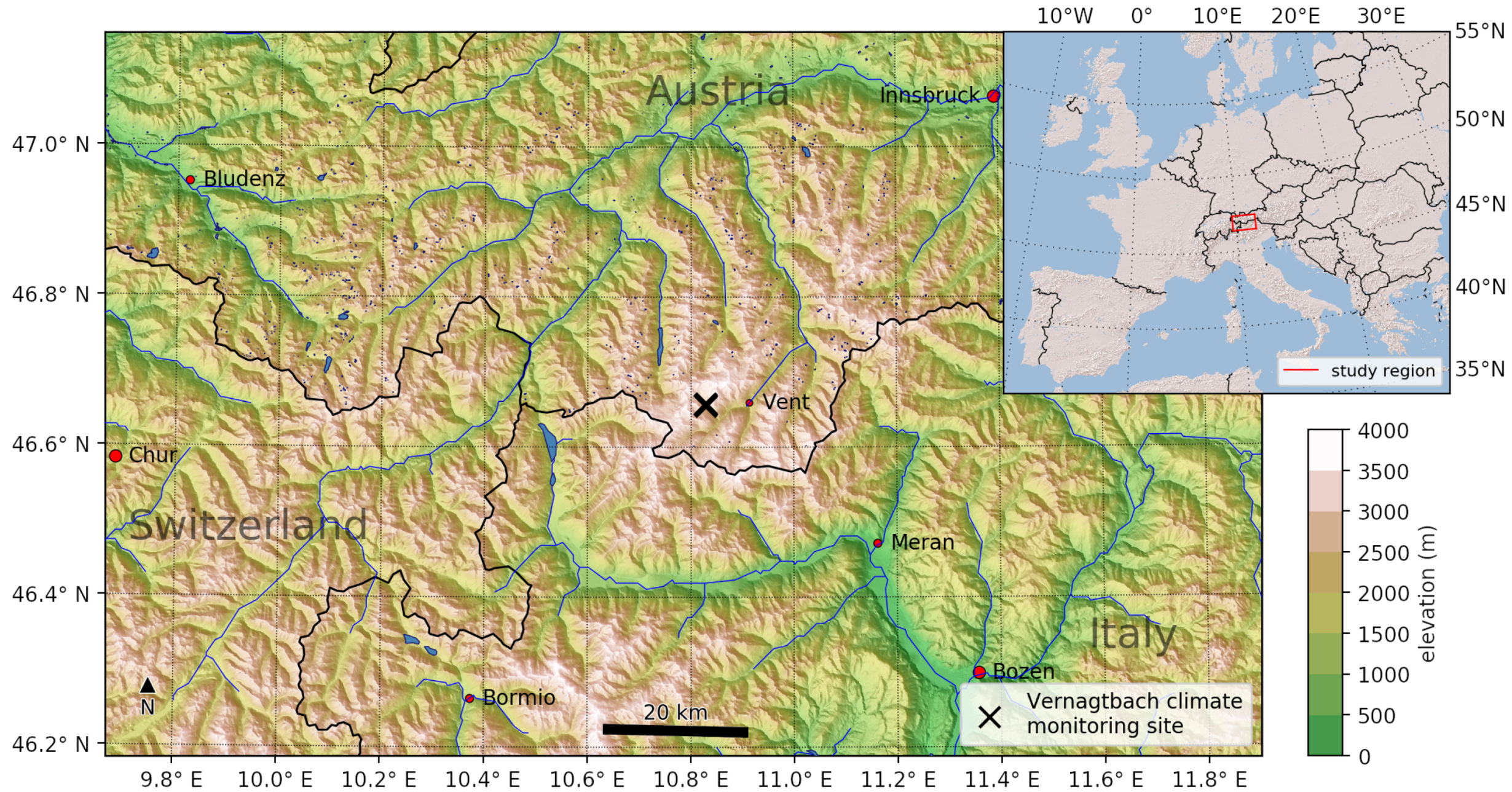
2.1. The Vernagtbach Climate Monitoring Site (VERNAGT)

The Vernagtbach climate monitoring site, hereafter referred to as VERNAGT, is located at 2640 MSL in the Vernagtbach glacier basin in the Austrian European Alps (see Figure 1). The European Alps are a 1200 km long, approximately 200 km wide and up to 4800 MSL high mountain range, characterized by strong spatial gradients of weather and climate [32]. VERNAGT is situated in an inner alpine dry valley close to the main alpine crest that includes peaks above 3000 MSL. The mean annual precipitation at VERNAGT is about 1500 mm [33]. VERNAGT is surrounded by rocky terrain, with a distance of about 1500 m to the glacier terminus in 2012 [34]. When VERNAGT was installed in fall 1973 as part of a long-term glacier monitoring programme, the glacier terminus was at a distance of approximately 1000 m from the station [35]. Since then, VERNAGT has undergone several revisions that were necessary to adapt to changes in the discharge conditions of the Vernagtbach, measurement techniques and the available funding [4,36]. VERNAGT data considered in this study cover the period 1979 to 2012 and were downloaded by PANGAEA (Data Publisher for Earth and Environmental Science, https://pangaea.de/). For the analysis in this study, VERNAGT observations downloaded as five-minutes centered averages were converted to daily means (only for days with complete records) and to annual and seasonal means (with a maximum of five days of missing data allowed for each year or season). Data gaps mostly affect the winter and spring time series, when the measurement devices were buried under snow. Thus, within the twenty-three years long true evaluation period, there are eleven annual mean values, twenty-two autumn mean values, eleven winter mean values, fourteen spring mean values, and twenty-three summer mean values available.

2.2. sDoG: Statistically Postprocessing Reanalysis Data to the Station Scale (One-Dimensional)

This study applies the statistical downscaling method sDoG (statistical Downscaling for Glacierized mountain environments) [23,24]. sDoG is a statistical postprocessor of reanalysis data originally developed for glacierized mountain environments. The statistical procedures underlying sDoG, however, are not limited to glacierized mountain environments and can, in principle, be applied for any site of interest. sDoG adjusts reanalysis data to in situ meteorological observations to more accurately represent station-scale atmospheric conditions. The overarching goal of sDoG is to extend short, typically few years long weather station records to multidecade long records in the past, similar in concept to the studies by [37,38]. sDoG is designed to consider the pitfalls of fitting limited, often patchy weather station data. The minimum possible length of an observational time series as input for sDoG has been identified as approximately three years [23]. Next to the length of the observational time series, observation quality plays a key role in the development of skillful models with sDoG. Measurement errors deleteriously impact the model training, but the sDoG algorithm is designed to detect these problems. Low performance quantified in the double cross-validation procedure employed by sDoG can be either an indication of low predictive power of the coarse-scale predictors or a symptom of measurement errors [23,24].

In contrast to most downscaling methods, sDoG is applicable only to reanalysis data and not to freely running climate models as predictors, because it uses information about the time sequencing in the observations for fitting the statistical relationships [39,40]. sDoG, in contrast to the vast majority of downscaling studies, thus profits from the advantages of numerical weather prediction postprocessing techniques, i.e., generally shorter time series can be used for model training, and cross-validation can be applied for assessing the model accuracy. Downscaling of free running climate models, in contrast, is limited to correct long-term distributional aspects, and it is not recommended to use cross-validation for assessing the performance of these models [21]. Currently, and as presented in this study, the sDoG code is one-dimensional—that is, applicable to only one site and one atmospheric quantity; thus, sDoG does not consider intersite and intervariable correlations. sDoG is written in MATLAB and it is available as a bitbucket repository (https://bitbucket.org/MarlisH/sdog/src/master/).

A crucial element of sDoG is the predictor selection, i.e., the selection of the information from the reanalysis data set that is important for the quantity of interest [24]. Note that in its current version, sDoG applies ERA-Interim data as predictors, with the adaptation of sDoG to include ERA5 being under way. For the dimensionality reduction in the predictor space, sDoG combines least-squares regression with the Least Absolute Shrinkage and Selection Operator, LASSO [41]. Note that next to least-squares regression, generalized linear models and symmetry producing variable transformations are available options in sDoG (e.g., for precipitation). The sDoG model for VERNAGT air temperature in this study is based on a systematic analysis of different predictor options performed by the authors of [24]. More precisely, the authors of [24] compared the efficiency of using predictor information either in terms of horizontal fields of a single atmospheric quantity (G), a single atmospheric quantity at different vertical levels (L), different atmospheric quantities at one level and one grid point (V), or combinations thereof: horizontal fields of different atmospheric quantities (GV), or different atmospheric quantities on different vertical levels (VL) or horizontal fields of a variable at different levels (GL). This analysis was repeated for different sites (including VERNAGT) and atmospheric quantities individually for each day of year. The results of [24] showed high dependence of the model skill on the applied predictor option and the importance of using different predictors for different days of year. The analysis also revealed cases for which larger predictor data sets yielded lower model skill. In other words, considering more information in the modeling procedure did not necessarily improve the results, as found particularly the in case of limited observation quality [24]. For more information on the predictor selection algorithm, see [24].

The sDoG core includes a double cross-validation procedure with an inner loop for model selection and an outer loop for uncertainty estimation. The cross-validation considers serial correlation by applying a buffer (determined by the autocorrelation function) between training and evaluation observations (moving block cross-validation). Like the predictor selection, the double cross-validation procedure is performed for each day of the year separately. The development of different functional relationships for different days of the year is more sophisticated than combining seasonal standardization with a single model for the entire year, because the latter method does not account for seasonality in the model error [24]. sDoG calculates one and two standard error estimates for each day of the year by assuming a Gaussian distribution of the cross-validation-based test error. More precisely, the one standard error (1SE) is defined as the standard deviation of the cross-validation-based test error, and the two standard error (2SE) is defined as the 95th percentile of the cross-validation-based test error. Significance testing of the skill of the developed relationships is based on the moving block bootstrap; for details, see [24].

The authors of [24] applied sDoG for daily precipitation, air temperature, relative humidity, wind speed and solar radiation at three sites, all located in complex terrain in the close proximity to mountain glaciers: next to VERNAGT, the Mount Brewster measuring site in the Southern Alps of New Zealand, and the Artesonraju measuring site in the tropical South American Andes. Of all sites and assessed variables, the most successful model was obtained for VERNAGT air temperature, with the lowest uncertainty and the highest skill scores exceeding 0.9 for the entire year [24]. For other variables/sites, e.g., for precipitation at VERNAGT or for air temperature at the Artesonraju measuring site, sDoG shows larger cross-validation-based uncertainty estimates presumably related to shortcomings of the observations [24]. In this study, sDoG was used for the first time to extend an observational time series beyond the model training/cross-validation period. Furthermore, the sDoG performance was evaluated at various time scales beyond the daily time scale of the model training. We focus on VERNAGT air temperature in a true verification setting, to address potential problems of sDoG not identified by the cross-validation procedure (best-case scenario).

2.3. Evaluation Strategy

Decade-long measurement series such as those available from VERNAGT are exceptional for remote mountain sites. The true verification performed in this study consisted of the following steps. First, sDoG was trained using data from 2002 to 2012 only. Then, sDoG produced a retrospective forecast of daily air temperature at VERNAGT for the period from 1979 to 2001. Finally, the sDoG retrospective forecast was evaluated based on VERNAGT observations from 1979 to 2001. In the remainder of this paper, the term “obs-training” refers to VERNAGT observations from 2002 to 2012, and “obs-trueval” refers to the VERNAGT observations over the true evaluation period 1979 to 2001 (

Table 1. Short names and details for the reference data sets considered in this study. All reference data sets were bias corrected based on obs-training (bc); see Equation (3). The altitude (MSL) refers to the height of the surface topography for the coordinates corresponding to VERNAGT.

Short Name	Data Set	MSL	Period	Grid	Reference
ERA-Interim	ERA-Interim 750 hPa air temperature (bc)	1750 m	1979–2019	80 km	[45]
ERA5	ERA5 750 hPa air temperature (bc)	2426 m	1979–pres	31 km	[12]
ERA5-Land	ERA5-Land 2 m air temperature (bc)	2871 m	1981–pres	9 km	[12]
HARMONIE	HARMONIE 2 m air temperature (bc)	2710 m	1961–pres	11 km	[46]
MESCAN-SURFEX	UERRA MESCAN-SURFEX 2 m air temperature (bc)	2817 m	1961–2019	5.5 km	[14]
ALARO	CORDEX ALARO-0 2 m air temperature (bc)	2843 m	1979–2010	12.5 km	[47]
Vent	Vent station 2 m air temperature (bc)	1905 m	1935–pres	point	[48]
SPARTACUS	SPARTACUS 2 m air temperature (bc)	2941 m	1961–2012	1 km	[8]

). The evaluation focused on various time scales (day-to-day, seasonal, annual, season-cycle), and thus explicitly distinguished between calibrated and not calibrated aspects. Furthermore, added value of sDoG was quantified over alternative data sets (listed below). The comparison of sDoG to reference data sets not only shed more light on the potential of sDoG, but also added information for users with respect to each individual reference data set for VERNAGT. Along with the retrospective forecast, sDoG delivers cross-validation-based uncertainty estimates in terms of confidence intervals. The true evaluation performed in this study offers the possibility to test the validity of cross-validation by testing if the cross-validation-based uncertainty estimates (based on obs-training) hold for the true evaluation period.

Added value of the sDoG retrospective forecast over each of the reference data sets is calculated as percentage improvement (or reduction of error, RE). RE is calculated here after [42]:

$$RE=100·SS,$$

(1)

with

$$SS=1-\overline{ϵ{\left(t\right)}^2}/\overline{{ϵ}_{\mathrm{r}}{\left(t\right)}^2}.$$

(2)

$SS$ is the mean squared error (MSE)-based skill score [43]. The term $\overline{ϵ{\left(t\right)}^2}$ is the MSE of the model to be evaluated (here, sDoG), and $\overline{{ϵ}_{\mathrm{r}}{\left(t\right)}^2}$ is the MSE of a given reference model. In this study, errors are calculated as differences between sDoG and the reference data sets (Table 1) to the VERNAGT observations from 1979 to 2001 (obs-trueval) at all considered time scales. Note that the range of RE is $(-\infty ,100]$. A RE of sDoG close to zero thus implies that the performance of sDoG is similar to the performance of the reference data sets. A RE of sDoG close to 100% means that the term $\overline{ϵ{\left(t\right)}^2}/\overline{{ϵ}_{\mathrm{r}}{\left(t\right)}^2}$ tends to zero and thus that sDoG clearly outperforms the reference data set. Negative values of RE cannot be interpreted in terms of percentage reduction of error, but they imply that the errors of sDoG are larger than the errors of the reference data set. RE thus quantifies if and how much sDoG adds value over all reference data sets considered here.

Application of Equations (1) and (2) for different temporal scales is performed here as follows. $ϵ\left(t\right)$ is calculated as the difference between obs-trueval and sDoG, and ${ϵ}_{\mathrm{r}}\left(t\right)$ as the difference between obs-trueval and each reference data set with the time series aggregated to each of the investigated time scales. The investigated time scales are (1) the overall daily time scale including all types of variability (daily, seasonal, and year-to-year), (2) day-to-day variability (corresponding to the overall daily time scale with the seasonal cycle and the year-to-year variations removed), (3) the 23-years mean seasonal cycle (thus, 365 values) and (4) year-to-year variations and season-to-season variations (with absolute values removed). This way, values of RE can be assigned to the different modes of variability considered in their calculation.

The significance of RE is tested based on the moving block bootstrap [24]. The moving block bootstrap procedure considers differences of the effective sample size for the different time scales investigated in this study [44]. In practice, it is more difficult to prove significance of RE values if the underlying error time series have few values and/or are affected by serial correlation because this reduces the effective sample size [44]. For example, for the annual, winter, spring, summer and autumn time series, only 11, 11, 13, 22 and 23 values of obs-trueval are available for the calculation of RE, respectively. Note also that differences in RE between different reference data sets are not tested here for significance, but can be interpreted in terms of “no added value” of one reference data set with a larger RE value over another with a smaller RE value. Smaller (larger) RE values of sDoG at a given time scale imply smaller (larger) MSEs, and thus errors of the reference data sets, respectively.

The true verification setting in this study allows us to verify the cross-validation-based uncertainty estimates 1SE and 2SE. 1SE and 2SE are the 68% (1SE) and 95% (2SE) confidence intervals of the sDoG retrospective forecast, estimated as standard deviation (1SE) and 95 percentile (2SE) of the test error based on cross-validation in the training period. The evaluation of 1SE and 2SE is performed by counting the portion of obs-trueval that effectively fall within sDoG ± 1SE and sDoG ± 2SE. This analysis is shown individually for each year, and on average over the true evaluation period. If the resulting portion exceeds 68% in case of sDoG ± 1SE and 95% in case of sDoG ± 2SE, this indicates that 1SE and 2SE estimated here by cross-validation underestimate the true uncertainties found in the evaluation period.

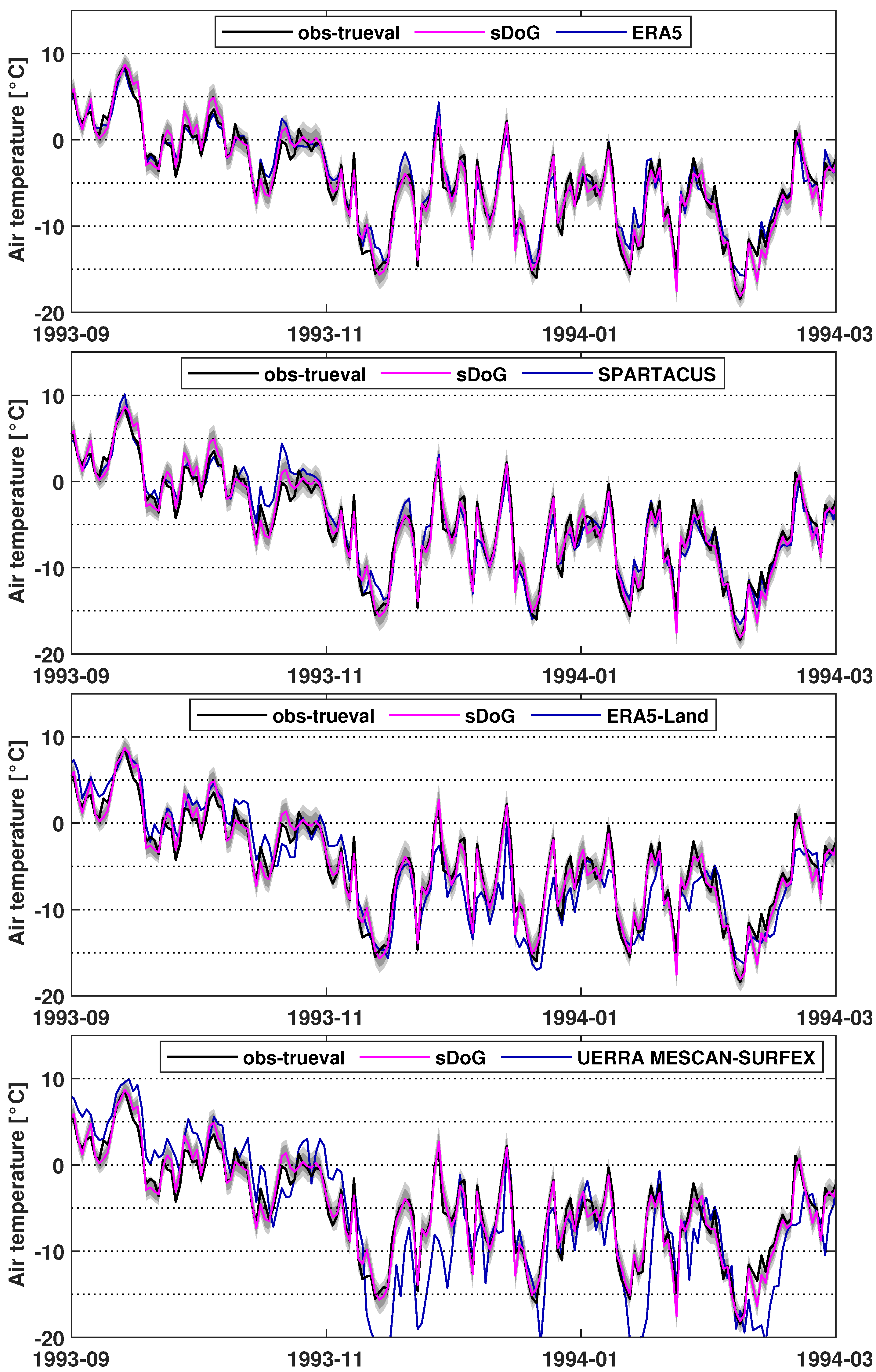
2.4. The Reference Data Sets

Table 1 details the reference data sets used to benchmark the performance of sDoG in this study. Firstly, different types of reanalysis products are considered, including ERA-Interim (predictors of sDoG), available globally at approximately 80 km horizontal resolution and from 1979 to August 2019 [45]; ERA5, the newest reanalysis data set by the ECMWF on a 30 km grid (globally) available from 1979 to present [12]; ERA5-Land, a replay of the land component of ERA5 at 9 km horizontal resolution, extending back to 1981; the regional reanalysis UERRA HARMONIE on a 11 km grid available for the European domain from 1961 to present [46], and UERRA MESCAN-SURFEX data set, a land surface analysis of HARMONIE at 5.5 km horizontal resolution [14]. Furthermore, a regional climate model simulation of the past observed climate is considered, namely ALARO-0 within the CORDEX initiative driven by ERA-Interim at the initial and lateral boundaries and available at 12.5 km horizontal resolution (0.11${}^{°}$) from 1979 to 2010 [47]. Finally, two reference data sets based only on observations are included, namely SPARTACUS, a 1 km gridded air temperature data set based on quality controlled observations for Austria available from 1961 to present [8], and the air temperature time series of a station located at only four kilometers distance to VERNAGT: Vent station (indicated in Figure 1). Note that Vent station was not involved in the generation of SPARTACUS.

For data available on pressure levels, like ERA-Interim and ERA5, there are two options of extracting air temperature for a site of interest, (1) 2 m air temperature or (2) air temperature from the pressure level corresponding to the site. In a preliminary analysis for this study, we tested both 2 m air temperature and 750 hPa air temperature by ERA-Interim for VERNAGT (pressure at VERNAGT varies around 740 hPa), and found 750 hPa air temperature outperforming 2 m air temperature concerning all considered aspects (not shown). In the remainder of this study, we therefore show results only for 750 hPa air temperature for both ERA-Interim and ERA5. For all other reference data sets (not available on pressure levels), 2 m air temperature is used (see also

Table 2. Overview about the added value of sDoG over all considered reference data sets and at all considered time scales in the true evaluation period. The first column shows the biases of all reference data sets and sDoG (last row) to obs-trueval (true evaluation observations from 1979 to 2001). The values in brackets are the biases of the reference data sets without bias correction, thus including the altitude bias. The remaining columns show the added value in terms of reduction of error RE (Equation (1)) of sDoG over all assessed reference data sets (top to bottom) at different time scales (left to right). Values of RE not found to be significantly positive (at a 5% significance level) are shown in brackets. Negative scores are given for completeness, but are not equivalent to RE of a reference data set over sDoG, because the range of RE is $(-\infty ,1]$ see [42].

	Mean Bias [${}^{°}$C]	Reduction of Error RE of sDoG (%)
Short-name		overall	day-to-day	seasonal cycle	year-to-year
(see Table 1)					annual	SON	DJF	MAM	JJA
obs-training	0.62	-	-	-	-	-	-	-	-
ERA-Interim	0.12 (1.15)	56	26	76	55	(15)	61	(16)	(–17)
ERA5	0.28 (0.7)	40	24	(41)	74	42	56	(9)	(–8)
ERA5-Land	0.58 (–2.38)	83	61	94	91	79	(31)	66	(27)
HARMONIE	–0.10 (–1.76)	81	66	93	63	72	58	65	(–49)
MESCAN-SURFEX	–0.62 (–4.12)	94	91	98	98	96	98	88	(35)
ALARO	0.18 (–0.89)	90	88	90	94	94	92	89	75
Vent	0.24 (3.87)	68	52	85	67	66	(43)	(22)	(–14)
SPARTACUS	0.09 (–2.25)	50	44	(8)	(8)	38	(28)	(0)	(–33)
sDoG	0.21	-	-	-	-	-	-	-	-

). Note that ERA-Interim on pressure levels outperforming ERA-Interim surface data was also pointed out for VERNAGT, and for two other high mountain sites in New Zealand and Peru [24]. For all gridded reference data sets except SPARTACUS, the four closest grid points are bilinearly interpolated to the study site’s coordinates. For SPARTACUS, the closest grid point is considered.

Due to the high topographic complexity around VERNAGT, none of the reference data sets corresponds to the altitude of the site exactly (see Table 1). Even for SPARTACUS on a 1 km grid, a height difference of about 300 m remains to VERNAGT. The 750 hPa pressure level considered in the case of ERA-Interim and ERA5 does not correspond exactly to the altitude of VERNAGT. Thus, all reference data sets suffer from an altitudinal bias in some form due to the atmospheric lapse rate (Table 2, bias values in brackets). It is beyond the scope of this study to seek an observation-independent altitude adjustment for all reference data sets. However, to isolate the performance of the reference data sets for each temporal aspect addressed here from the altitude bias that would otherwise obliterate the results, all reference data sets (RD) are standardized ($bc$) to the mean of obs-training, as follows:

$${\mathrm{RD}}_{bc}\left(t\right)=\mathrm{RD}\left(t\right)-\overline{\mathrm{RD}(2002–2012)}+\overline{\mathrm{obs}-\mathrm{training}},$$

(3)

with $\overline{\mathrm{RD}(2002–2012)}$ being the temporal mean of a reference data set over the period 2002 to 2012, and $\overline{\mathrm{obs}-\mathrm{training}}$ the temporal mean of obs-training. This way, all reference data sets “have seen” VERNAGT observations, but are still independent of obs-trueval, like sDoG. In this study, no additional correction for a misrepresentation of the seasonal cycle in the reference data sets is applied. However, in the calculation of RE values for the year-to-year and season-to-season variability, absolute values are removed, and thus the general and seasonal offsets in the reference models are eliminated automatically. Seasonal offsets are then evaluated explicitly with the evaluation of the 23-years mean seasonal cycle. This way, we clearly distinguish between the performance in representing year-to-year variability and the performance in simulating the seasonal cycle correctly.

3. Results

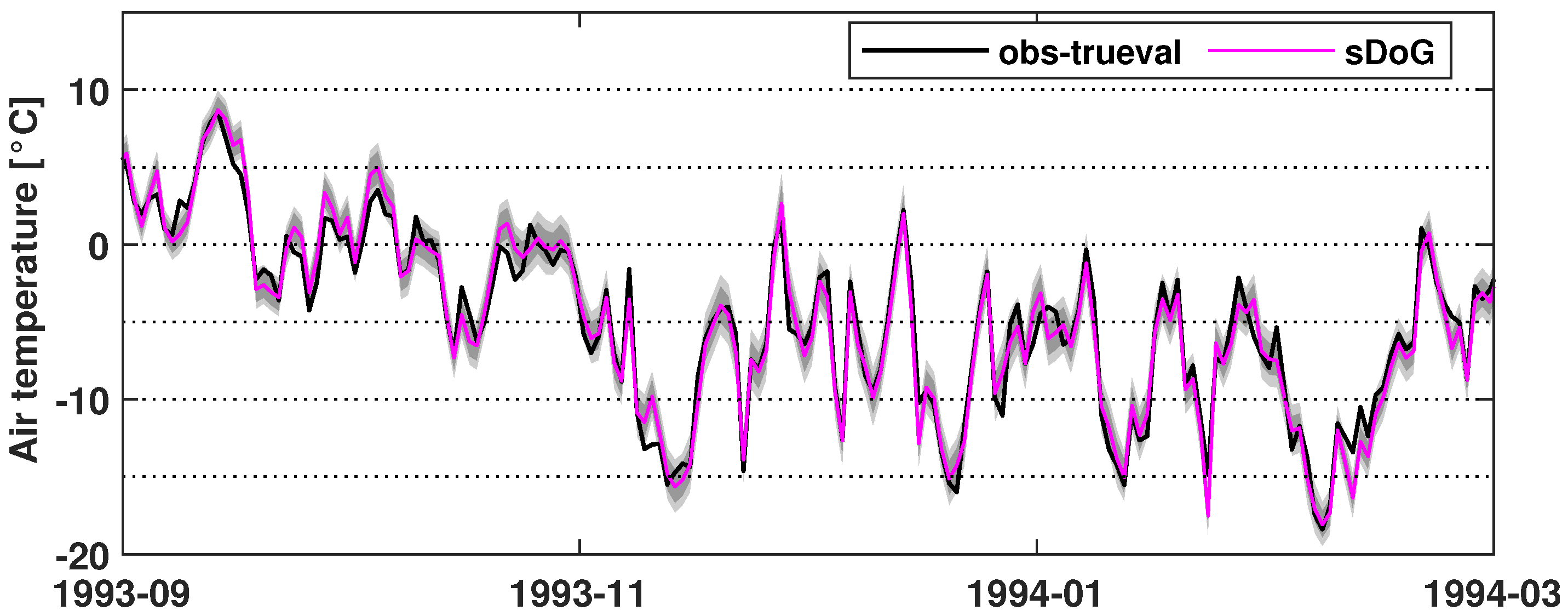
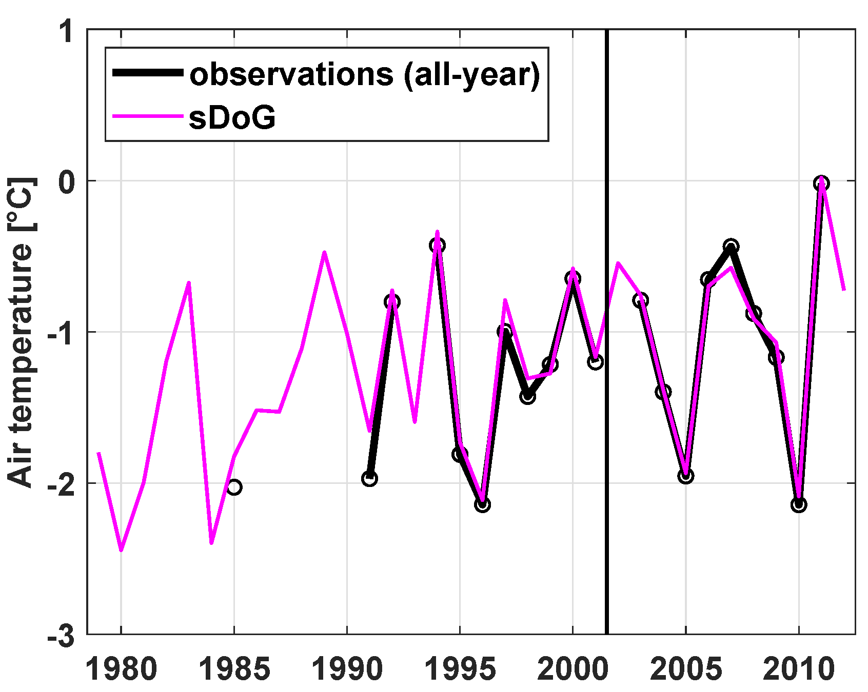
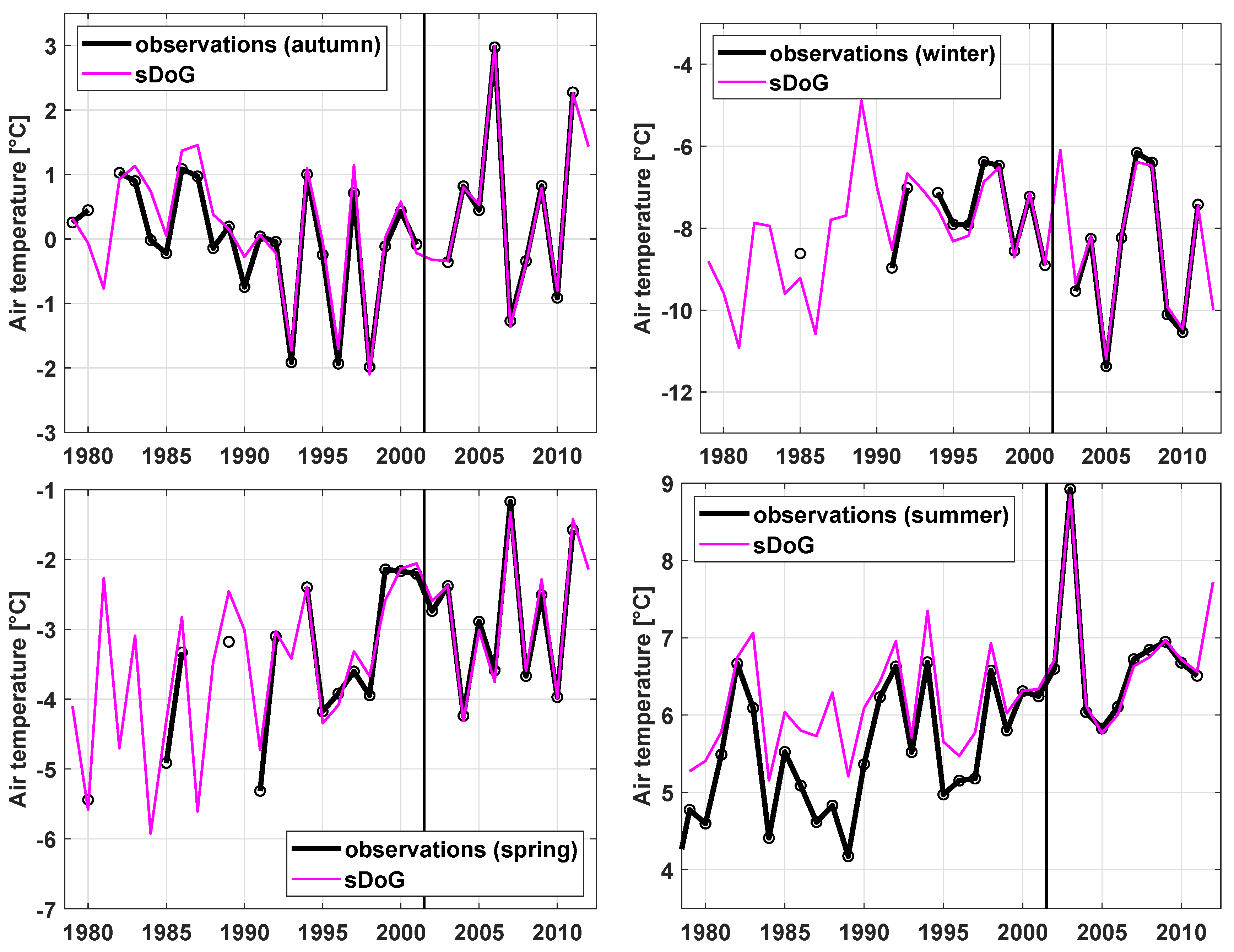
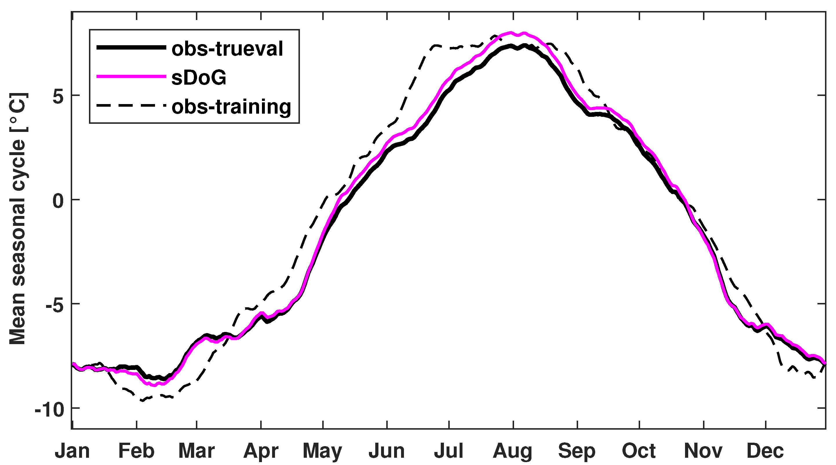
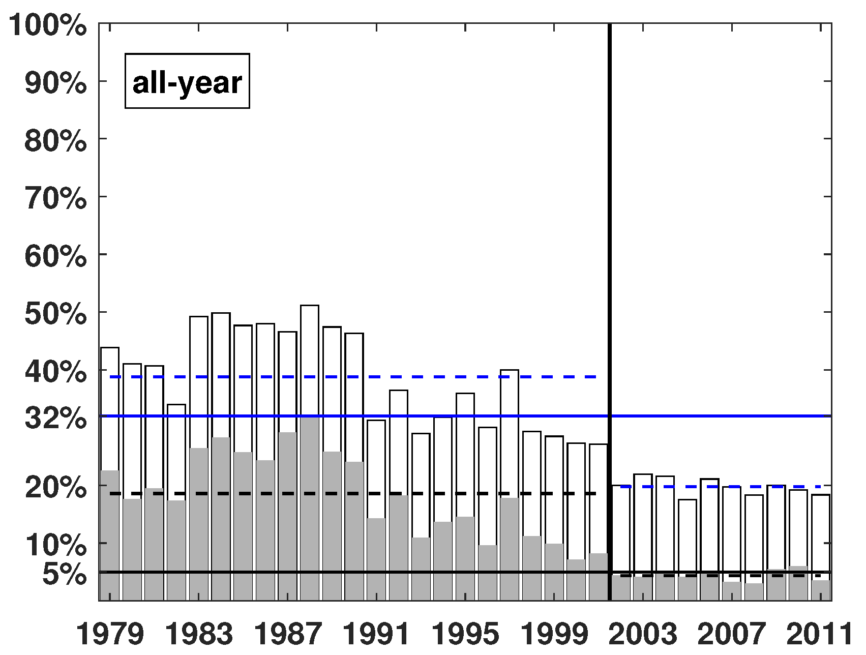
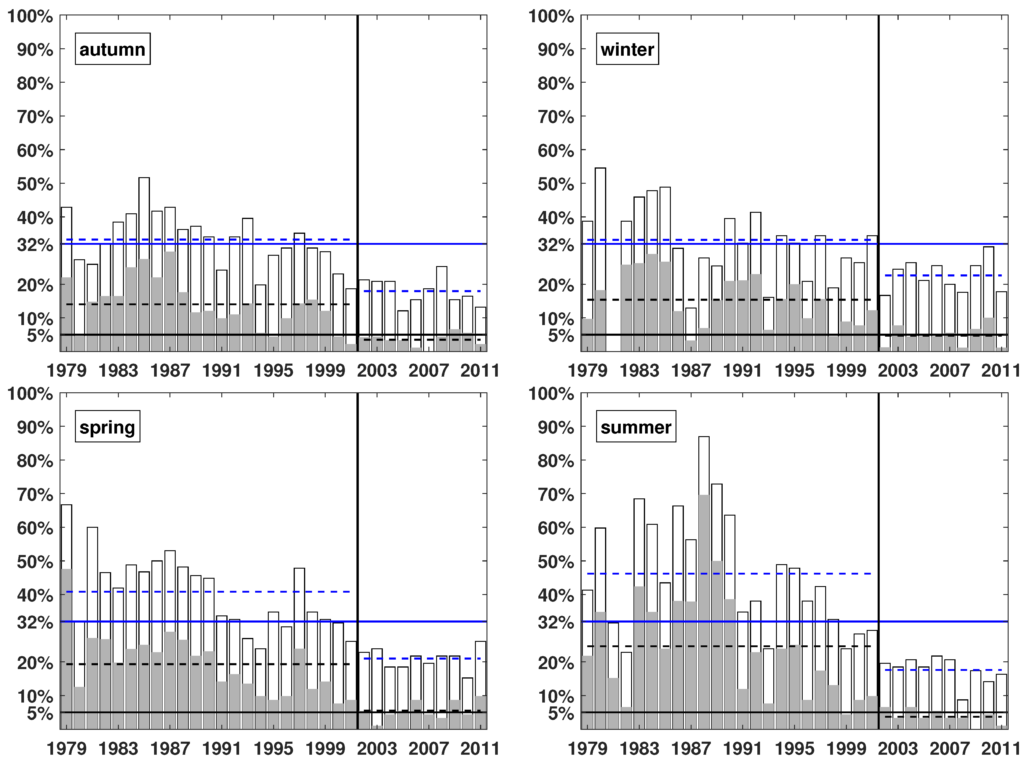
3.1. sDoG Performance at Different Time Scales

Figure 2 shows an arbitrarily selected, six-months-long snapshot of VERNAGT air temperature daily means in the beginning of the true evaluation period. Shown are the measurements together with the sDoG retrospective forecast. Figure 2 shows that sDoG is in close agreement with the observations. The differences between sDoG and obs-trueval are small compared to the overall variability of the time series. For the displayed time window, there is a temperature range of more than 25 ${}^{°}$C. Figure 3 and Figure 4 show year-to-year variations of the annual and seasonal temperatures at VERNAGT: obs-trueval (1979–2001), obs-training (2002–2012) and sDoG (1979–2012). Mean annual temperatures at VERNAGT have a range of about 2 ${}^{°}$C, while the seasonal temperatures (autumn, winter, spring and summer) have a range of about 5 ${}^{°}$C. sDoG corresponds well to obs-training for all seasons (see Figure 3 and Figure 4, post-2002). This is not a matter because sDoG is trained to daily values which show much larger variations than the annual values (see [26]). In the true evaluation period, errors between sDoG and obs-trueval are smallest for the autumn time series, with the mean absolute error amounting to 0.2 ${}^{°}$C. The largest errors are found for the summer time series, with a mean absolute error of 0.38 ${}^{°}$C. For the summer time series in particular, the errors between sDoG and obs-trueval are larger in the true earlier evaluation period than in the later evaluation period and they are systematically positive; sDoG simulates too warm summers. In the evaluation of the overall daily time series (e.g., in Figure 2), this bias is masked, because variability at the daily time scale is much larger.

Figure 5 compares the mean annual cycle of air temperature at VERNAGT over the true evaluation period as measured (obs-trueval) with the sDoG retrospective forecast. The mean annual cycle in obs-trueval ranges from –8 ${}^{°}$C to +7 ${}^{°}$C. The annual cycle averaged over the training period (obs-training) is also shown. sDoG corresponds closely to obs-trueval, with smaller errors in winter than in summer, where sDoG systematically overestimates obs-trueval with errors up to 0.6 ${}^{°}$C. Differences between obs-trueval and obs-training, by contrast, exceed 3 ${}^{°}$C for some days of the year, are positive from April through November and negative for winter and early spring. The differences between sDoG and obs-trueval being much smaller than the differences between sDoG and obs-training indicate that sDoG is well trained without overfit and that the predictors are meaningful. Also, while obs-training is lower than obs-trueval throughout the winter months December to February, sDoG slightly overestimates December temperatures, is almost identical to obs-trueval in January and slightly underestimates obs-trueval in February. Thus, although the overall variability in the time series used for training is much larger than the annual cycle (compare, e.g., Figure 2 and Figure 5), sDoG is able to capture changes of the mean seasonal cycles from obs-training to obs-trueval. The overall bias between sDoG and obs-trueval is 0.21 ${}^{°}$C (see Table 2), and between obs-trueval and obs-training 0.62 ${}^{°}$C. sDoG is thus able to correct obs-training towards obs-trueval, but the remaining bias is still in an order of magnitude relevant for trend detection (e.g., [49]).

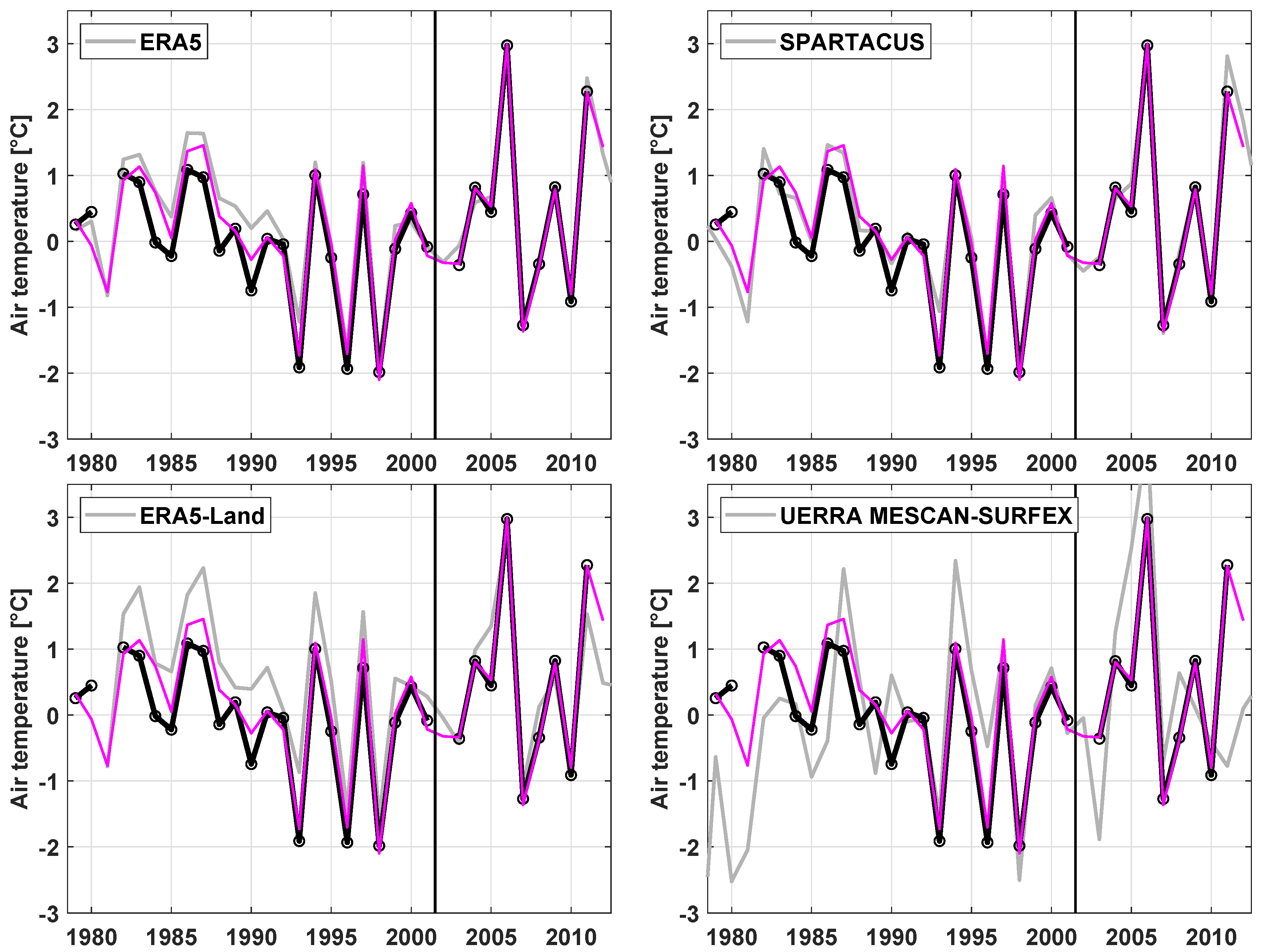
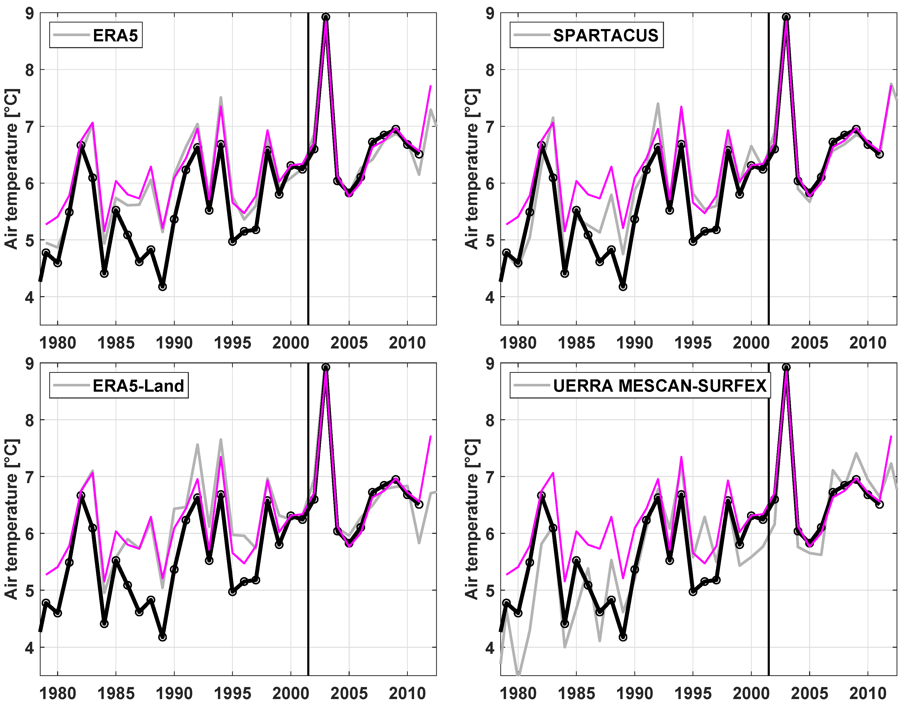
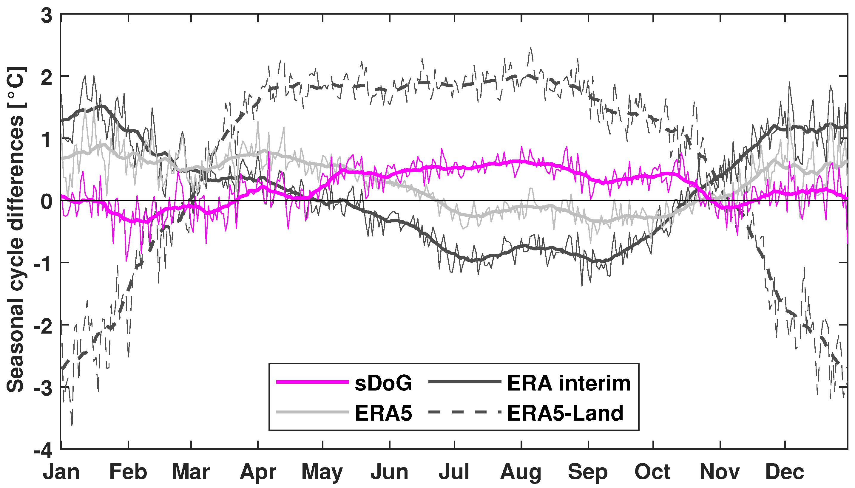
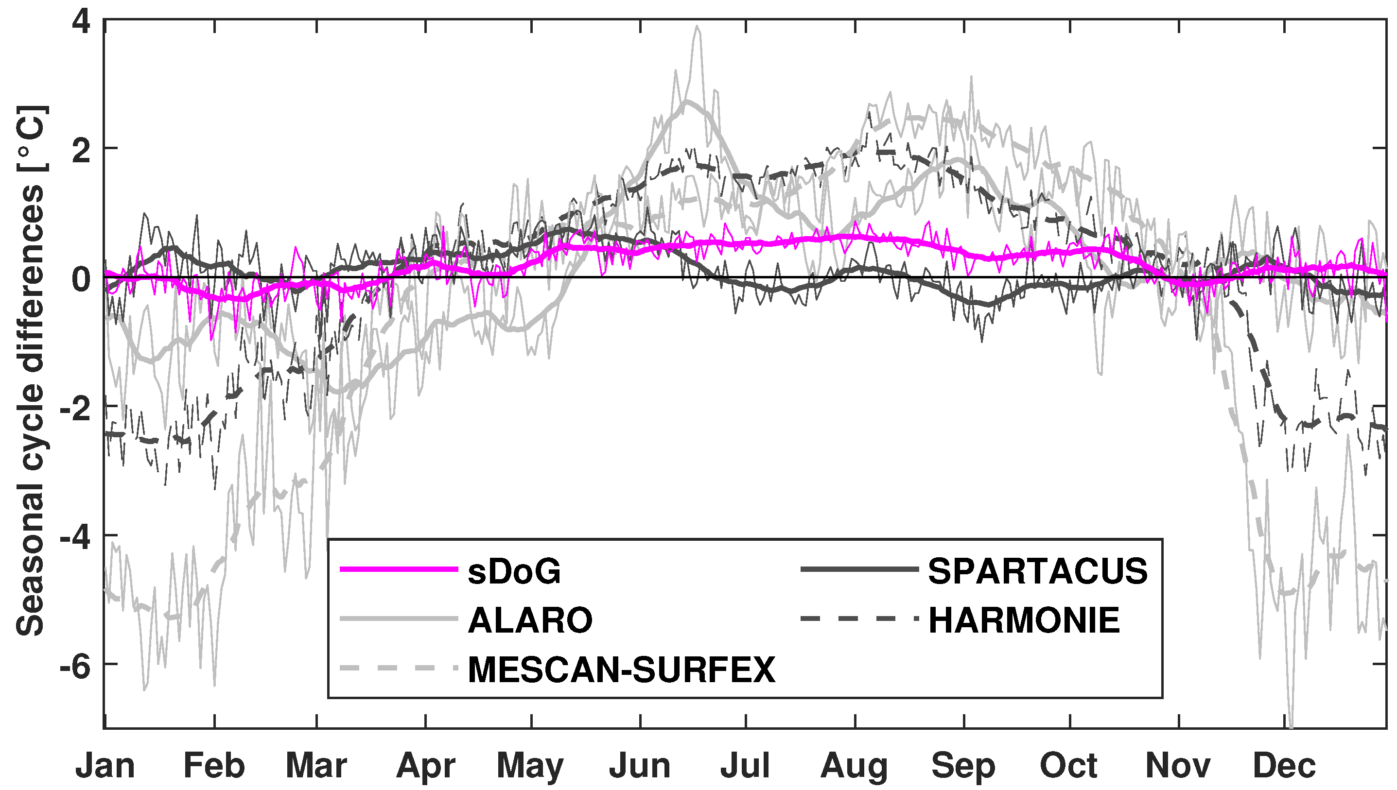
3.2. Added Value of sDoG Over the Reference Data Sets

In this section, the performance of sDoG in the true evaluation period is compared to the performance of the reference data sets listed in Table 1. Table 2 shows values of RE of sDoG over all considered reference data sets at all considered time scales. Furthermore, Figure 6 shows a snapshot of daily air temperatures at VERNAGT in the earlier true evaluation period together with sDoG, ERA5, SPARTACUS, ERA5-Land and MESCAN-SURFEX. The selection of reference data sets reflects the range of RE values, from low (ERA5 and SPARTACUS), intermediate (ERA5-Land), and high values of RE (MESCAN-SURFEX, see also Table 2). Figure 7 and Figure 8 show autumn and summer time series with the same selection of reference data sets. Figure 9 and Figure 10 show differences between the mean seasonal cycles averaged over the true evaluation period of all reference data sets to obs-trueval. How does the performance of sDoG compare to the performances of available alternative data sets, and how do the considered data sets perform amongst each other?

RE values of sDoG are significantly positive over all reference data sets for the overall daily values (i.e., daily values including seasonal cycle and year-to-year variations) and the day-to-day variations (i.e., daily values with seasonal cycle and year-to-year variations removed). RE ranges from 24% for the best performing reference data set (ERA5) to 90% for the reference data sets with the largest errors (MESCAN-SURFEX). Regarding year-to-year variations, values of RE of sDoG are positive over all reference data sets for the annual, autumn, winter and spring time series, ranging from 0 (SPARTACUS spring time series) to 98% (MESCAN-SURFEX annual and winter time series), but are not significantly positive for all reference data sets. Failing to prove significance for the annual, autumn, winter and spring time series is also related to the fact that less values are available for the calculation of RE values than for the other time scales. Concerning the summer time series, values of RE of sDoG are positive over only three out of seven considered reference data sets, and significantly positive in only one case (ALARO). Concerning the representation of the seasonal cycle, values of RE of sDoG are significantly positive over all reference data sets except for SPARTACUS and ERA5. Failing to prove significance of RE of sDoG over ERA5 even though the value of RE amounts 41% relates to the high serial correlation of the season cycle time series that reduces the effective sample size in the significance estimation see [42].

When comparing the performance amongst the reference data sets, ERA5 is the best reference data set regarding the daily time scale (with and without seasonal cycle and year-to-year variations), and SPARTACUS is the best reference data set regarding the seasonal cycle and year-to-year variations (see Table 2 and Figure 6, Figure 7, Figure 8 and Figure 9). Note also that while ERA5 and ERA-Interim show problems in modeling summer air temperatures similarly as sDoG, SPARTACUS captures the observed variations in the first part of the true evaluation period more closely. Regarding day-to-day variability, by contrast, ERA5 and ERA-Interim show slightly higher performances than SPARTACUS (e.g., Figure 6). ERA-Interim outperforms ERA5 concerning year-to-year variations and shows a performance very close to ERA5 concerning day-to-day variability, but improvement of ERA5 over ERA-Interim is evident in the representation of the seasonal cycle (see also Figure 10). SPARTACUS clearly outperforms Vent at all considered time aspects.

Overall, the best performing reference data sets are SPARTACUS, ERA5 and ERA-Interim, and the reference data sets with the worst performance are ERA5-Land, HARMONIE, ALARO and MESCAN-SURFEX. Note also that the differences of RE values within the best performing reference data sets are small compared to the differences of RE values between the best and the worst performing reference data sets. In other words, the performances of SPARTACUS, ERA5 and ERA-Interim are comparably similar, while there is a larger gap to the performances of ERA5-Land, HARMONIE, ALARO, and MESCAN-SURFEX. In fact, values of RE of sDoG over ERA5-Land, HARMONIE, ALARO and MESCAN-SURFEX range up to 94% for the overall day-to-day, up to 91% for the day-to-day isolated variations, up to 98% for the seasonal cycle, and up to 98% for year-to-year variations. Only for the winter time series, ERA5-Land outperforms ERA5 as well as ERA-Interim. Within the worst performing reference data sets, ERA5-Land and HARMONIE outperform ALARO and MESCAN-SURFEX. MESCAN-SURFEX, the only product that includes two numerical-model-based downscaling steps, shows the lowest performance.

To sum up, the two global reanalysis products ERA5 and ERA-Interim outperform the higher-resolution, numerical-model-based downscaling products ERA5-Land, HARMONIE, MESCAN-SURFEX and ALARO. For the numerical-model-based downscaling products considered here, these results do not support the assumption of added value over their coarse scale drivers (e.g., [19]). However, sDoG applied to the coarsest scale reference data set considered here (ERA-Interim) clearly outperforms ERA-Interim and all higher-resolution reference data sets for all time aspects despite summer air temperature variability.

3.3. Verification of the Cross-Validation-Based Uncertainty Estimates of sDoG

Figure 11 and Figure 12 demonstrate the verification of the cross-validation-based uncertainty estimates 1SE and 2SE, the 68% and 95% confidence intervals of sDoG, respectively. More precisely, for each year in the true evaluation period, the percentages of values of obs-trueval exceeding sDoG ± 1SE and sDoG ± 2SE (e.g., illustrated as dark and light grey shaded areas in Figure 2 and Figure 6) are shown. The analysis performed at a daily time scale is shown for all data (Figure 11), and for data stratified to the individual seasons (Figure 12), to investigate how the shortcomings of the cross-validation-based estimates of 1SE and 2SE relate to each season. Figure 12 shows that sDoG uncertainties are more realistic for the autumn and winter seasons than for spring and summer. In fact for autumn and winter, the cross-validation-based 1SE almost fits the true 1SE, including over the entire true evaluation period, on average 66.7% and 66.8% of the data. For spring and summer by contrast, the 1SE estimate includes only 59% and 54% of the true evaluation data, respectively. Also evident in Figure 11 and Figure 12 is that the cross-validation-based 1SE estimate is more realistic than the cross-validation-based 2SE estimate: for autumn and winter, the 2SE estimate includes 85% and 86% of the true evaluation data, and for spring and summer the 2SE estimate includes 81% and 75%. Furthermore, sDoG 1SE and 2SE estimates are more often exceeded in the first part of the true evaluation period (1979 to 1990, more distant to the training period), than in the later true evaluation period (1991 to 2001). This is evident in the annual data (Figure 11), but particularly for the spring and summer seasons (Figure 12).

In the training period, the 1SE and 2SE estimates overestimate the true errors (see Figure 11 and Figure 12: dashed black and blue lines are below the solid black and blue lines post 2001). This is because 1SE and 2SE are calculated from the cross-validation-based test errors. The difference between the solid and black lines in the training period shows the merit of the applied cross-validation procedure: it shifts the error estimates from the errors in the training period towards more realistic values.

4. Discussion and Conclusions

sDoG is a one-dimensional downscaling model designed to extend short-term weather station data from high mountain sites to the baseline climate. This study evaluates sDoG and its cross-validation-based uncertainty estimates for daily air temperature at the Vernagtbach climate monitoring site (2640 MSL in the European Alps). sDoG is trained and cross-validated using data from 2002 to 2012, while the evaluation considers data from 1979 to 2001. The results show that sDoG adds significant value over various reference data sets available for the study area in the true evaluation period at very distinct spatial resolutions, including global and regional reanalysis data sets (ERA-Interim, ERA5, ERA5-Land, UERRA HARMONIE, UERRA MESCAN-SURFEX), regional climate model output (historical simulation of the model ALARO-0 by the CORDEX initiative), and a 1 km-resolution gridded observation-based product available for the territory of Austria (SPARTACUS).

Added value of sDoG is demonstrated over all reference data sets at all considered time scales (day-to-day, seasonal cycle, and year-to-year). Problems of sDoG, however, emerge in the modeling of summer air temperatures, for which added value of sDoG is positive over only three out of eight reference data sets, and significant in only one case. This comparably poor performance of sDoG is most likely related to a nonstationarity of the microclimate of the Vernagtbach climate monitoring site that violates the stationarity assumption underlying sDoG. More precisely, throughout the evaluation period the Vernagtferner (glacier) terminus formerly close to the site retreated several hundred meters leaving behind rocky moraine terrain. Overall, the glacierized area in the region around the Vernagtbach climate monitoring site diminished (e.g., [34,35]). This nonstationarity of the microclimate is more important for spring and summer than for autumn and winter, and affects sDoG in an order of magnitude relevant for trend analysis (e.g., [49]). In the case of the Vernagtbach climate monitoring site the changes of the surrounding microclimate are well documented (e.g., [34,35,36]. This information is not yet considered in the sDoG modeling procedure, which next to the training observations uses only reanalysis data predictors. An avenue for further developing sDoG not investigated in this study could be to consider metadata available for the entire forecasting period (e.g., distance of the station to the glacier terminus) as predictors in the downscaling procedure.

Evaluation of the cross-validation-based standard errors of sDoG (daily values) shows that the one standard error, 1SE (68 percentile) is more accurately modeled than the two standard error, 2SE (95 percentile). Discrepancies of the cross-validation-based 1SE to the true 1SE affect mostly daily values in summer and spring and in the first part of the true evaluation period (i.e., prior to 1990). For the autumn and winter time series, by contrast, the cross-validation-based 1SE is very close to the true 1SE throughout the true evaluation period. Discrepancies are however more important concerning 2SE. The cross-validation-based 2SE underestimates the true 2SE throughout the true evaluation period and for all seasons. The underlying cause of this underestimation might be that the cross-validation sample (twelve years) is too short for an accurate determination of the 95% confidence interval of sDoG. This affects the applicability of sDoG for the analysis of extreme values. Further investigation is needed to determine the minimum amount of data required to accurately determine 2SE based on cross-validation, when the stationarity assumption is satisfied.

Next to the validation of sDoG, this study also offers a detailed, station-scale evaluation and comparison of all considered reference data sets. The evaluation of all reference data sets is performed after applying a very basic downscaling step to remove an average altitude bias. Without this bias correction, the altitude bias would dominate the evaluation of all considered reference data sets as even for the highest resolution data sets the altitude bias remains important. In practice, the simple bias correction proposed in this study has the same prerequisite like sDoG: a few-yearly observational time series of the site needs to be available. For sites without observations, removing the altitude bias is intricate because the thermal vertical profiles are known to vary locally and seasonally (e.g., [2]). Removing the altitude bias using pressure level information is an option for the data sets available on pressure levels (e.g., reanalysis data), but this step assumes that the lapse rate extracted by the coarse-scale data set is accurate.

The best performing reference data sets in this study are SPARTACUS, ERA5, and ERA-Interim. Concerning day-to-day and year-to-year variations, the performances of ERA5 and ERA-Interim are very similar, but ERA5 shows improvement over ERA-Interim in the representation of the 23-year mean seasonal cycle. The gridded observations-product SPARTACUS clearly outperforms the weather station Vent (at only four kilometers distance to the Vernagtbach climate monitoring site) for all considered time aspects. This hints at the sophistication of the air temperature interpolation algorithm underlying SPARTACUS and the added value of the gridded, quality controlled product even at a station scale see [2,8]. ERA5-Land is a surface analysis of ERA5 at 9 km (versus 31 km of ERA5) grid resolution. Our study, however, cannot evidence added value of ERA5-Land over ERA5 for air temperature at the Vernagtbach climate monitoring site. ERA5-Land shows larger mean squared errors than ERA5 (and also ERA-Interim) for all time scales except the winter time series. Similarly, the regional reanalysis HARMONIE at 11 km resolution does not show added value over its driving data set ERA-Interim at 80 km grid resolution. Even more underwhelming is the performance of the MESCAN-SURFEX, a 5.5 km grid surface analysis applied to HARMONIE. MESCAN-SURFEX shows the largest mean squared errors of all reference data sets at all considered time aspects. This performance drawback of MESCAN-SURFEX cannot be related to insufficient spatial resolution or dislocation. In fact, the performance differences between ERA-Interim and ERA5 (89 km versus 31 km grid) are small compared to the performance differences between both ERA-Interim and ERA5 to MESCAN-SURFEX (89 and 31 km versus 5.5 km grid). We also find the CORDEX ALARO simulation showing weaker performance than the driving data ERA-Interim for all considered time aspects. This must be contrasted to the lack of added value for MESCAN-SURFEX, ERA5-Land, and HARMONIE, because ALARO is run as freely evolving climate simulation constrained by ERA-Interim only at the lateral boundaries throughout the simulation period. Thus, added value is not to be expected concerning time sequencing aspects [47]. However in the representation of the 23-year mean seasonal cycle ALARO conceptually should add value over ERA-Interim.

Even though our study is based on only one site, the accordance between the best performing reference data sets (SPARTACUS, ERA5 and ERA-Interim) albeit largely varying spatial resolutions, and their superior performance over several higher resolution data sets are noteworthy. A similar analysis as performed in this study but for more sites and different atmospheric quantities could shed a more general light onto the lack of added value of the investigated RCM-based data sets found here for air temperature at the Vernagtbach climate monitoring site. In fact, a general conclusion on the added value of numerical-model-based downscaling or regional climate modeling does not exist, since it is known that regional climate models can also amplify errors present in a global climate simulation (e.g., [50]).

While this study does not evaluate downscaling models other than sDoG, note that sDoG differs from most downscaling approaches in that it is not applicable to freely running climate models as predictors. This is because sDoG uses information about the time sequencing in the observations for fitting the statistical relationships, which enables the application of sDoG to relatively short time series. Furthermore, sDoG is different from most downscaling models as its goal is to extend and/or complement weather station data for past periods [37,38]. More precisely, sDoG aims for a reconstruction of baseline climates rather than knowledge about future climate change. The exploration of statistical downscaling methods to extend or complement interrupted station records—like sDoG—has been suggested also for the generation of long-term gridded observation-based products like SPARTACUS see [2]. Output by sDoG, however, provided a successful evaluation, can be used for the training of downscaling models that focus on future climate change, (e.g., as “pseudo-observations”). This also includes the present day evaluation and further development of kilometer-scale regional climate simulation runs (e.g., [16]). This way, sDoG could contribute to increase knowledge about future climate change for data-scarce high mountain regions. While our study sheds light onto benefits and shortcomings of sDoG and other state-of-art atmospheric data sets, it confirms once more the continued need of a reliable and dense in situ observational network for high mountain regions (e.g., [51]).

References

1. Pepin, N.C.; Lundquist, J.D. Temperature trends at high elevations: Patterns across the globe. Geophys. Res. Lett. 2008, 35. [Google Scholar] [CrossRef] [Green Version]
2. Frei, C. Interpolation of temperature in a mountainous region using nonlinear profiles and non-Euclidean distances. Int. J. Climatol. 2014, 1585–1605. [Google Scholar] [CrossRef]
3. Isotta, F.A.; Begert, M.; Frei, C. Long-Term Consistent Monthly Temperature and Precipitation Grid Data Sets for Switzerland Over the Past 150 Years. J. Geophys. Res. Atmos. 2019, 124, 3783–3799. [Google Scholar] [CrossRef]
4. Escher-Vetter, H.; Braun, L.N.; Siebers, M. Hydrological and Meteorological Records from the Vernagtferner Basin—Vernagtbach Station, for the Years 2002 to 2012. Available online: https://doi.pangaea.de/10.1594/PANGAEA.829516 (accessed on 2 October 2020).
5. Cullen, N.J.; Conway, J.P. A 22 month record of surface meteorology and energy balance from the ablation zone of Brewster Glacier, New Zealand. J. Glaciol. 2015, 61, 931–946. [Google Scholar] [CrossRef] [Green Version]
6. Carey, M. In the Shadow of Melting Glaciers. Climate Change and Andean Society; Oxford University Press: Oxford, UK, 2010; p. 288. [Google Scholar]
7. Juen, I. Glacier Mass Balance and Runoff in the Cordillera Blanca, Peru. Ph.D. Thesis, University of Innsbruck, Innsbruck, Austria, 2006. [Google Scholar]
8. Hiebl, J.; Frei, C. Daily temperature grids for Austria since 1961—Concept, creation and applicability. Theor. Appl. Climatol. 2016, 124, 161–178. [Google Scholar] [CrossRef]
9. Werner, A.T.; Schnorbus, M.A.; Shrestha, R.R.; Cannon, A.J.; Zwiers, F.W.; Dayon, G.; Anslow, F. A long-term, temporally consistent, gridded daily meteorological dataset for northwestern North America. Sci. Data 2019, 6. [Google Scholar] [CrossRef] [PubMed] [Green Version]
10. Kalnay, E.; Kanamitsu, M.; Kistler, R.; Collins, W.; Deaven, D.; Gandin, L.; Iredell, M.; Saha, S.; White, G.; Woollen, J.; et al. The NCEP/NCAR 40-Year Reanalysis Project. Bull. Am. Meteorol. Soc. 1996, 77, 437–471. [Google Scholar] [CrossRef] [Green Version]
11. Rienecker, M.M.; Suarez, M.J.; Gelaro, R.; Todling, R.; Bacmeister, J.; Liu, E.; Bosilovich, M.G.; Schubert, S.D.; Takacs, L.; Kim, G.K.; et al. MERRA: NASA’s modern-era retrospective analysis for research and applications. J. Clim. 2011, 24, 3624–3648. [Google Scholar] [CrossRef]
12. Hersbach, H.; Bell, W.; Berrisford, P.; Horányi, A.; Sabater, J.M.; Nicolas, J.; Radu, R.; Schepers, D.; Simmons, A.; Soci, C.; et al. Global Reanalysis: Goodbye ERA-Interim, Hello ERA5; The European Centre for Medium-Range Weather Forecasts: Reading, UK, 2019; pp. 17–24. [Google Scholar] [CrossRef]
13. Kaiser-Weiss, A.K.; Borsche, M.; Niermann, D.; Kaspar, F.; Lussana, C.; Isotta, F.A.; van den Besselaar, E.; van der Schrier, G.; Undén, P. Added value of regional reanalyses for climatological applications. Environ. Res. Commun. 2019, 1, 071004. [Google Scholar] [CrossRef]
14. Bazile, E.; Abida, R.; Verrelle, A.; Le Moigne, P.; Szczypta, C. Report for the 55 Years MESCAN-SURFEX Re-Analysis; Technical Report; Météo-France/CNRS: Toulouse, France, 2017. [Google Scholar]
15. Giorgi, F.; Jones, C.; Asrar, G. Addressing climate information needs at the regional level: The CORDEX framework. WMO Bull. 2009, 58, 175–183. [Google Scholar]
16. Shi, X.; Chow, F.K.; Street, R.L.; Bryan, G.H. Key Elements of Turbulence Closures for Simulating Deep Convection at Kilometer-Scale Resolution. J. Adv. Model. Earth Syst. 2019, 11, 818–838. [Google Scholar] [CrossRef] [Green Version]
17. Kotlarski, S.; Keuler, K.; Christensen, O.B.; Colette, A.; Déqué, M.; Gobiet, A.; Goergen, K.; Jacob, D.; Lüthi, D.; van Meijgaard, E.; et al. Regional climate modeling on European scales: A joint standard evaluation of the EURO-CORDEX RCM ensemble. Geosci. Model Dev. 2014, 7, 1297–1333. [Google Scholar] [CrossRef] [Green Version]
18. Foley, A.; Kelman, I. EURO-CORDEX regional climate model simulation of precipitation on Scottish islands (1971–2000): Model performance and implications for decision-making in topographically complex regions. Int. J. Climatol. 2018, 38, 1087–1095. [Google Scholar] [CrossRef] [Green Version]
19. Di Luca, A.; de Elía, R.; Laprise, R. Challenges in the Quest for Added Value of Regional Cloate Dynamical Downscaling. Curr. Clim. Chang. Rep. 2015, 1, 10–21. [Google Scholar] [CrossRef]
20. Maraun, D.; Wetterhall, F.; Ireson, A.M.; Chandler, R.E.; Kendon, E.J.; Widmann, M.; Brienen, S.; Rust, H.W.; Sauter, T.; Themeßl, M.; et al. Precipitation downscaling under climate change. Recent developments to bridge the gap between dynamical models and the end user. Rev. Geophys. 2010, 48. [Google Scholar] [CrossRef]
21. Maraun, D.; Shepherd, T.G.; Widmann, M.; Zappa, G.; Walton, D.; Gutiérrez, J.M.; Hagemann, S.; Richter, I.; Soares, P.M.M.; Hall, A.; et al. Towards process-informed bias correction of climate change simulations. Nat. Clim. Chang. 2017, 7, 764–773. [Google Scholar] [CrossRef] [Green Version]
22. Michaelsen, J. Cross-validation in statistical climate forecast models. J. Clim. Appl. Meteorol. 1987, 26, 1589–1600. [Google Scholar] [CrossRef] [Green Version]
23. Hofer, M.; Marzeion, B.; Mölg, T. A statistical downscaling method for daily air temperature in data-sparse, glaciated mountain environments. Geosci. Model Dev. 2015, 8, 579–593. [Google Scholar] [CrossRef] [Green Version]
24. Hofer, M.; Nemec, J.; Cullen, N.J.; Weber, M. Evaluating Predictor Strategies for Regression-Based Downscaling with a Focus on Glacierized Mountain Environments. J. Appl. Meteorol. Climatol. 2017, 56, 1707–1729. [Google Scholar] [CrossRef]
25. Maraun, D.; Widmann, M. Cross-validation of bias-corrected climate simulations is misleading. Hydrol. Earth Syst. Sci. 2018, 22, 4867–4873. [Google Scholar] [CrossRef] [Green Version]
26. Haerter, J.; Hagemann, S.; Moseley, C.; Piani, C. Climate model bias correction and the role of timescales. Hydrol. Earth Syst. Sci. 2011, 15, 1065–1073. [Google Scholar] [CrossRef] [Green Version]
27. Ehret, U.; Zehe, E.; Wulfmeyer, V.; Warrach-Sagi, K.; Liebert, J. HESS Opinions “Should we apply bias correction to global and regional climate model data?”. Hydrol. Earth Syst. Sci. 2012, 16, 3391–3404. [Google Scholar] [CrossRef] [Green Version]
28. Hewitson, B.C.; Daron, J.; Crane, R.G.; Zermoglio, M.F.; Jack, C. Interrogating empirical-statistical downscaling. Clim. Chang. 2014, 122, 539–554. [Google Scholar] [CrossRef] [Green Version]
29. Dixon, K.W.; Lanzante, J.R.; Nath, M.J.; Hayhoe, K.; Stoner, A.; Radhakrishnan, A.; Balaji, V.; Gaitán, C.F. Evaluating the stationarity assumption in statistically downscaled climate projections: Is past performance an indicator of future results? Clim. Chang. 2016, 135, 395–408. [Google Scholar] [CrossRef] [Green Version]
30. Barsugli, J.J.; Guentchev, G.; Horton, R.M.; Wood, A.; Mearns, L.O.; Liang, X.Z.; Winkler, J.A.; Dixon, K.; Hayhoe, K.; Rood, R.B.; et al. The Practitioner’s Dilemma: How to Assess the Credibility of Downscaled Climate Projections. Eos Trans. Am. Geophys. Union 2013, 94, 424–425. [Google Scholar] [CrossRef] [Green Version]
31. Erlandsen, H.B.; Parding, K.M.; Benestad, R.; Mezghani, A.; Pontoppidan, M. A hybrid downscaling approach for future temperature and precipitation change. J. Appl. Meteorol. Climatol. 2020, 1–46. [Google Scholar] [CrossRef]
32. Schmidli, J.; Schmutz, C.; Frei, C.; Wanner, H.; Schär, C. Mesoscale precipitation variability in the region of the European Alps during the 20th century. Int. J. Climatol. 2002, 22, 1049–1074. [Google Scholar] [CrossRef]
33. Braun, L.N.; Escher-Vetter, H.; Siebers, M.; Weber, M. Water Balance of the highly Glaciated Vernagt Basin, Ötztal Alps; chapter The Water Balance of the Alps; Innsbruck University Press: Innsbruck, Austria, 2007; Volume 3, pp. 33–42. [Google Scholar]
34. Rissel, R. Physikalische Interpretation des Temperatur-Index-Verfahrens zur Berechnung der Eisschmelze am Vernagtferner. Bachelor’s Thesis, Technische Universität Braunschweig, Fakultät Architektur Bauingenieurwesen und Umweltwissenschaften, Braunschweig, Germang, 2012. [Google Scholar]
35. Charalampidis, C.; Fischer, A.; Kuhn, M.; Lambrecht, A.; Mayer, C.; Thomaidis, K.; Weber, M. Mass-Budget Anomalies and Geometry Signals of Three Austrian Glaciers. Front. Earth Sci. 2018, 6, 218. [Google Scholar] [CrossRef]
36. Escher-Vetter, H.; Oerter, H.; Reinwarth, O.; Braun, L.N.; Weber, M. Hydrological and Meteorological Records from the Vernagtferner Basin—Vernagtbach Station, for the Years 1970 to 2001; PANGAEA: Bremen, Germany, 2012. [Google Scholar] [CrossRef]
37. Schneider, T. Analysis of Incomplete Climate Data: Estimation of Mean Values and Covariance Matrices and Imputation of Missing Values. J. Clim. 2001, 14, 853–871. [Google Scholar] [CrossRef]
38. Sansom, J.; Tait, A. Estimation of long-term climate information at location with short-term data records. J. Appl. Meteorol. 2003, 43, 915–923. [Google Scholar] [CrossRef]
39. Castro, C.L.; Pielke, R.A., Sr.; Leoncini, G. Dynamical downscaling: Assessment of value retained and added using the Regional Atmospheric Modeling System (RAMS). J. Geophys. Res. Atmos. 2005, 110. [Google Scholar] [CrossRef]
40. Pielke, R.A., Sr.; Wilby, R.L. Regional climate downscaling: What’s the point? Eos Trans. Am. Geophys. Union 2012, 93, 52–53. [Google Scholar] [CrossRef]
41. Hastie, T.; Tibshirani, R.; Friedman, J. The Elements of Statistical Learning: Data Mining, Inference, and Prediction, 2nd ed.; Springer Series in Statistics; Springer: New York, NY, USA, 2009; p. 533. [Google Scholar]
42. Wilks, D. Statistical Methods in the Atmospheric Sciences, 3rd ed.; International Geophysics; Elsevier Science: Amsterdam, The Netherlands, 2011; p. 704. [Google Scholar]
43. Murphy, A.H. Skill Scores Based on the Mean Square Error and Their Relationships to the Correlation Coefficient. Mon. Weather Rev. 1988, 116, 2417–2424. [Google Scholar] [CrossRef]
44. Wilks, D.S. Resampling hypothesis tests for autocorrelated fields. J. Clim. 1997, 10, 65–82. [Google Scholar] [CrossRef]
45. Dee, D.P.; Uppala, S.M.; Simmons, A.J.; Berrisford, P.; Poli, P.; Kobayashi, S.; Andrae, U.; Balmaseda, M.A.; Balsamo, G.; Bauer, P.; et al. The ERA-Interim reanalysis: Configuration and performance of the data assimilation system. Q. J. R. Meteorol. Soc. 2011, 137, 553–597. [Google Scholar] [CrossRef]
46. SMHI. UERRA Data User Guide v 3.0; Copernicus Climate Change Service Climate Data Store: Brussels, Belgium, 2019. [Google Scholar]
47. Giot, O.; Termonia, P.; Degrauwe, D.; De Troch, R.; Caluwaerts, S.; Smet, G.; Berckmans, J.; Deckmyn, A.; De Cruz, L.; De Meutter, P.; et al. Validation of the ALARO-0 model within the EURO-CORDEX framework. Geosci. Model Dev. 2016, 9, 1143–1152. [Google Scholar] [CrossRef] [Green Version]
48. Strasser, U.; Marke, T.; Braun, L.; Escher-Vetter, H.; Juen, I.; Kuhn, M.; Maussion, F.; Mayer, C.; Nicholson, L.; Niedertscheider, K.; et al. The Rofental: A high Alpine research basin (1890–3770 m a.s.l.) in the Ötztal Alps (Austria) with over 150 years of hydrometeorological and glaciological observations. Earth Syst. Sci. Data 2018, 10, 151–171. [Google Scholar] [CrossRef] [Green Version]
49. Thorne, P.W.; Lanzante, J.R.; Peterson, T.C.; Seidel, D.J.; Shine, K.P. Tropospheric temperature trends: History of an ongoing controversy. Wiley Interdiscip. Rev. Clim. Chang. 2011, 2, 66–88. [Google Scholar] [CrossRef]
50. Torma, C.; Giorgi, F.; Coppola, E. Added value of regional climate modeling over areas characterized by complex terrain. In Proceedings of the EGU General Assembly Conference Abstracts, EGU General Assembly Conference Abstracts, Vienna, Austria, 22–27 April 2015; p. 709. [Google Scholar] [CrossRef]
51. Scherrer, S.C. Temperature monitoring in mountain regions using reanalyses: Lessons from the Alps. Environ. Res. Lett. 2020, 15, 044005. [Google Scholar] [CrossRef]
Figure 1. Situation of the Vernagtbach climate monitoring site within the European Alps.
Atmosphere 11 01256 g001
Figure 2. Snapshot of daily air temperature at VERNAGT in the evaluation period: observations (obs-trueval, black), and the sDoG retrospective forecast (magenta) along with uncertainties; dark and light grey shadings are the one and two standard errors (1SE and 2SE).
Atmosphere 11 01256 g002
Figure 3. Annual mean air temperature at VERNAGT, observed (black) and modeled by sDoG (magenta) from 1979 to 2012. Note that due to data gaps in winter, observed values are missing particularly prior to 1990. The black vertical line separates the true evaluation period (1979 to 2001) from the training period (2002 to 2012).
Atmosphere 11 01256 g003
Figure 4. Seasonal mean air temperature at VERNAGT from 1979 to 2012, observations (black line with circles) and sDoG (magenta). Autumn (SON) air temperatures are shown in the top left panel, winter (DJF) in the top right panel, spring (MAM) in the bottom left panel and summer (JJA) in the bottom right panel. The black vertical line separates the evaluation period, obs-trueval (1979 to 2001) from the training period, obs-training (2002 to 2012). Note that while autumn (top left) and summer (bottom right) temperatures show almost complete records, winter (top right) and spring (bottom left) air temperatures are affected by missing data particularly prior to 1990.
Atmosphere 11 01256 g004
Figure 5. Mean seasonal cycle of VERNAGT air temperature: obs-trueval (black line), sDoG (true evaluation period, magenta) and obs-training (black dashed line). The seasonal cycles are calculated as moving average centered on each day of year with a window size of 20 days.
Atmosphere 11 01256 g005
Figure 6. Daily air temperature at VERNAGT: observations (black), the sDoG retrospective forecast (magenta) along with uncertainties (1SE and 2SE, dark and light grey shadings), and the reference data sets ERA5, SPARTACUS, ERA5-Land and UERRA MESCAN-SURFEX (blue). Shown is an arbitrarily selected snapshot in the true evaluation period.
Atmosphere 11 01256 g006
Figure 7. VERNAGT autumn (SON) air temperatures: observations (black), sDoG (magenta), and the reference data sets ERA5, SPARTACUS, ERA5-Land, and UERRA MESCAN-SURFEX (in grey). Note that for this figure the summer time series of the reference data sets are standardized to obs-training, because the emphasis is on season-to-season co-variability here (see Section 2.3). The performance in simulating the seasonal cycle is then illustrated separately in Figure 9 and Figure 10.
Atmosphere 11 01256 g007
Figure 8. VERNAGT summer (JJA) air temperatures: observations (black), sDoG (magenta), and the reference data sets ERA5, SPARTACUS, ERA5-Land and UERRA MESCAN-SURFEX (in grey). Note that for this figure the summer time series of the reference data sets are standardized to obs-training, because the emphasis is on season-to-season co-variability here (see Section 2.3). The performance in simulating the seasonal cycle is then illustrated separately in Figure 9 and Figure 10.
Atmosphere 11 01256 g008
Figure 9. Differences between the mean seasonal cycles of sDoG (magenta), ERA-Interim (dark grey), ERA5 (light grey) and ERA5-Land (grey dashed) to VERNAGT air temperature in the true evaluation period(1979-2001) (obs-trueval). Shown are the differences of the mean values calculated for each day of year (thin lines), and of moving averages centered on each day of year with a window size of 20 days (solid lines).
Atmosphere 11 01256 g009
Figure 10. Differences between the mean seasonal cycles of sDoG (magenta), SPARTACUS (dark grey), ALARO (light grey), HARMONIE (dark grey dashed) and UERRA MESCAN-SURFEX (light grey dashed) to VERNAGT air temperature in the true evaluation period (obs-trueval). Shown are the differences of the mean values calculated for each day of year (thin lines), and of moving averages centered on each day of year with a window size of 20 days (solid lines).
Atmosphere 11 01256 g010
Figure 11. Percentage of days for which the errors of sDoG exceed 1SE (white bars) and 2SE (grey bars). The black vertical line marks the end of the true evaluation period (1979 to 2001) and the beginning of the cross-validation period (2002 to 2012). Following the definition of 1SE and 2SE as 68% and 95% confidence intervals of sDoG, the white bars should on average not exceed 32% of the data (blue, upper solid line), and the grey bars should on average not exceed 5% of the data (black, lower solid line). The average of the white (grey) bars is indicated by the blue (black) dashed line individually for the true evaluation period and the training period, respectively. If the dashed lines are higher than the solid lines in the true evaluation period, this means that the cross-validation-based uncertainty estimates 1SE and 2SE underestimate the true uncertainties of sDoG.
Atmosphere 11 01256 g011
Figure 12. As Figure 11, but for autumn, winter, spring and summer. Limitations of the cross-validation procedure are particularly evident for the spring and summer seasons (see the larger gap between the dashed and the solid lines in the true evaluation period), and for the 95% confidence interval 2SE (because the gap between the black dashed and solid lines is larger than the gap between the blue dashed and solid lines).
Atmosphere 11 01256 g012