Source Apportionment of Aerosol at a Coastal Site and Relationships with Precipitation Chemistry: A Case Study over the Southeast United States

Abstract

This study focuses on the long-term aerosol and precipitation chemistry measurements from colocated monitoring sites in Southern Florida between 2013 and 2018. A positive matrix factorization (PMF) model identified six potential emission sources impacting the study area. The PMF model solution yielded the following source concentration profiles: (i) combustion; (ii) fresh sea salt; (iii) aged sea salt; (iv) secondary sulfate; (v) shipping emissions; and (vi) dust. Based on these results, concentration-weighted trajectory maps were developed to identify sources contributing to the PMF factors. Monthly mean precipitation pH values ranged from 4.98 to 5.58, being positively related to crustal species and negatively related to SO₄²⁻. Sea salt dominated wet deposition volume-weighted concentrations year-round without much variability in its mass fraction in contrast to stronger seasonal changes in PM_2.5 composition where fresh sea salt was far less influential. The highest mean annual deposition fluxes were attributed to Cl⁻, NO₃⁻, SO₄²⁻, and Na⁺ between April and October. Nitrate is strongly correlated with dust constituents (unlike sea salt) in precipitation samples, indicative of efficient partitioning to dust. Interrelationships between precipitation chemistry and aerosol species based on long-term surface data provide insight into aerosol–cloud–precipitation interactions.

1. Introduction

Aerosol–cloud interactions (ACI) are complex and not accurately represented by climate models [1]. These interactions remain the largest source of uncertainty in anthropogenic radiative forcing [2,3]. In contrast to subtropical regions characterized by stratocumulus decks such as off the western coasts of the United States (U.S.) [4], Chile [5], and Southern Africa (e.g., [6,7]), marine-related ACI studies are more scarce over the Western North Atlantic Ocean (WNAO) region [8].

Although few studies focusing on ACI over the WNAO have primarily relied on ship and/or aircraft data [8]. Even though these efforts have, in some cases, provided data at high temporal and spatial resolution and in the vicinity of clouds, downsides are the high cost, challenging logistics, and statistical limitations innate to short-term intensive campaigns. An alternative and indirect method to gain inferences about ACI is to use long-term data at surface monitoring networks gathering compositional data for precipitation and particulate matter. This method has been demonstrated for other regions such as an inland California site [9], the Southwestern U.S. [10], and Mexico City [11]. Those works demonstrated that colocated measurements of both precipitation and aerosol composition provide insight into some combination of the following processes: (i) the composition of particles serving as either the cloud condensation nuclei (CCN) or ice nuclei (IN) that eventually fall to the surface via wet deposition; (ii) uptake of species into existing droplets in cloud; and (iii) subcloud scavenging of different constituents. These three processes represent both aerosol effects on cloud (i) and cloud effects on aerosol (ii–iii). There are limitations when relating surface aerosol properties to precipitation at the same site, which are circumvented by airborne platforms flying around clouds; however, the ground-based approach leverages larger statistical datasets with broader temporal coverage that typically provide more speciation data.

For studies relating aerosol and precipitation chemistry, it helps to study locations with broad ranges in both aerosol and meteorological conditions. In this regard, coastal areas influenced by both natural and anthropogenic emissions are fitting as they are exposed to a wide assortment of aerosol types. On the western edge of the WNAO, Southern Florida fits into this category as it experiences influence from local and regional sources that are both biogenic and anthropogenic in nature [12], in addition to being under the impact of marine and shipping emissions [13], and long-range transport of dust [14] and smoke [15,16]. The area also experiences a wide range of precipitation, including from actively developing shallow cumulus clouds, which are common over the trade regions of most of the tropical oceans [17,18]. These clouds are especially important to study due to their radiative effect on climate model sensitivity [17]. Thunderstorms are prevalent during the summertime over the Gulf Coast and Florida, with the latter registering the highest concentration of thunderstorms in the U.S. [19]. Convergence from coastal sea breezes has been proposed as the dominant dynamic mechanism leading to thunderstorms during the summer months [20]. The combination of warm, moist maritime-tropical air and small-scale wind circulation (i.e., sea breeze) from both the Atlantic Ocean and the Gulf of Mexico provides the optimal conditions to form thunderstorms in this area.

Additionally, smaller bodies of water (e.g., Lake Okeechobee) can create circulations similar to sea breeze leading to conditions to form thunderstorms. Intercomparison of aerosol and wet deposition chemical data for Southern Florida can suggest what aerosol types participate in CCN/IN activation and what the resultant composition is of the wet deposition derived from clouds. Wet deposition flux magnitudes of different species are relevant for understanding impacts on surface ecosystems, which was already an active research area decades ago in the study region as part of the Florida Atmospheric Mercury Study [21,22].

This work aims to report on long-term aerosol and precipitation chemistry measurements from colocated monitoring sites at the Everglades National Park (NP) in Southern Florida. The analysis combined field measurement data, transport modeling, and source apportionment modeling to characterize the temporal trends and interrelationships between aerosol and precipitation chemistry from 2013 to 2018. The results and discussion are structured as follows: (i) summary of meteorological profile; (ii) sources of PM_2.5; (iii) precipitation chemistry profile; and (iv) interrelationships between precipitation and aerosol chemistry.

2. Methods

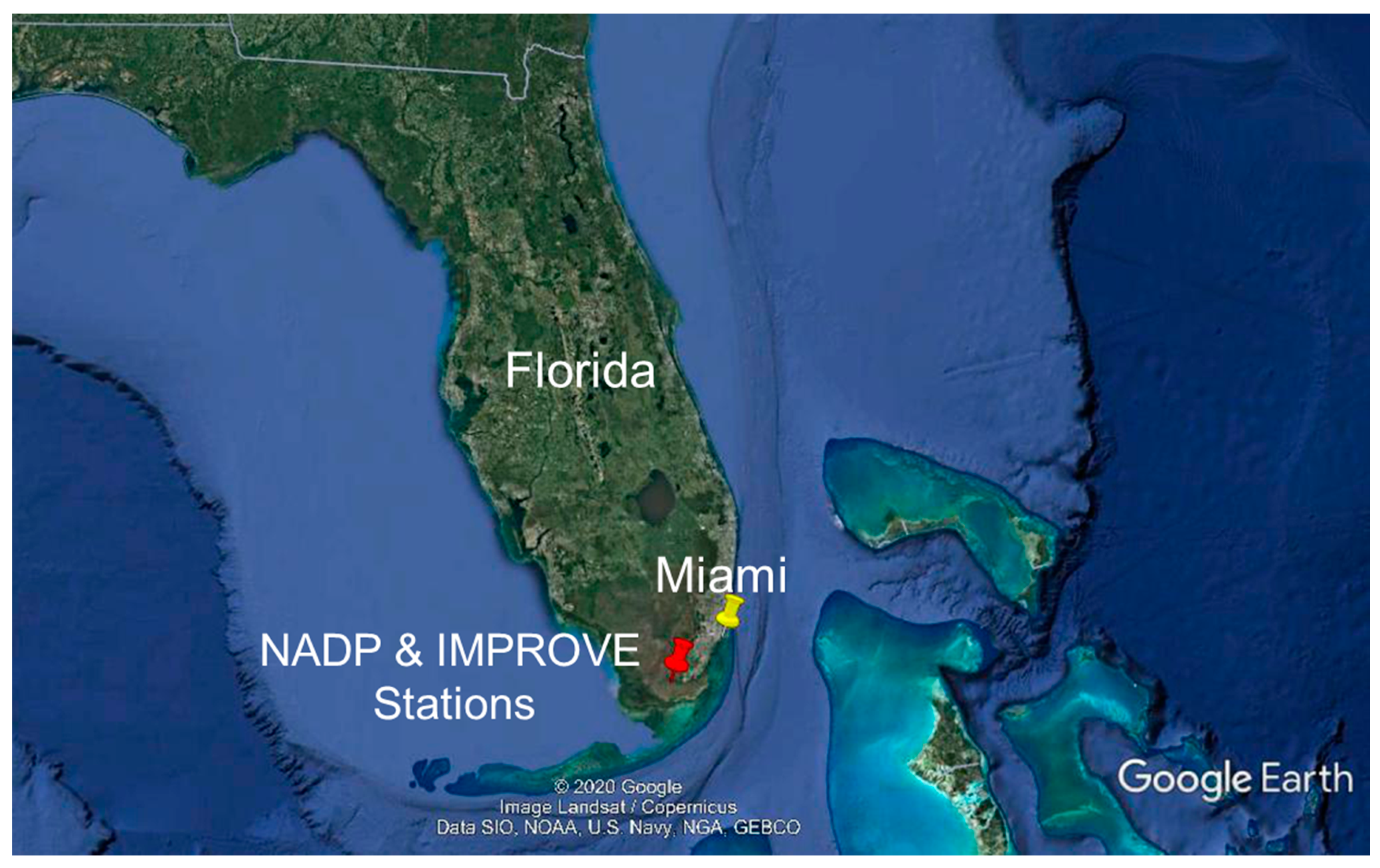
2.1. Site Description

The Everglades NP hosts the precipitation monitoring station (25.390° N 80.680° W, 2 m above sea level (m a.s.l.)) managed by the National Atmospheric Deposition Program/National Trends Network (NADP/NTN) and the Environmental Protection Agency (EPA) Interagency Monitoring of Protected Visual Environments (IMPROVE) aerosol monitoring station (25.391° N 80.6806° W, 1 m a.s.l.). Both sites are located approximately 25 km from the coast. The Everglades NP is a unique ecosystem formed by subtropical wetlands (Figure 1). Located approximately 90 km southwest of Miami (Miami-Dade County population = 2,761,581 for 2018) [23], Everglades NP extends 1.5 million acres across Southern Florida. Approximately 50% of the original area has been converted to agricultural land and urban development [24,25]. Currently, 397,000 acres around the Everglades NP and the southern tip of Lake Okeechobee area are used for commercial sugarcane crops, Florida’s most profitable crop [26]. A byproduct of sugarcane production is 7 million tons of dry sugarcane leaves that are removed and burnt before harvesting between October and late March [27]. This is a common practice in other sugarcane producing areas like Louisiana, U.S. [28], Cuba [29], and Brazil [30]. These activities consequently result in substantial biomass burning emissions [27,31].

2.2. Precipitation and Aerosol Composition

Established in 1977 by the U.S. State Agricultural Experiment Stations (SAES), the NADP/NTN (hereafter referred to as NADP) began monitoring wet deposition across the U.S. to measure its effects on the environment. The network continued to expand throughout the years and currently has over 260 sites with the Wisconsin State Laboratory of Hygiene at the University of Wisconsin-Madison as the NADP Program Office. In 1987, the IMPROVE program was set up with 30 monitoring sites located in national parks as part of the visibility monitoring network [32], which currently includes over 100 sites. This study’s data were retrieved from the NADP and IMPROVE stations located at the Everglades NP between January 2013 and December 2018.

The NADP site collected weekly precipitation samples for pH, conductance, and water-soluble ions concentrations (ammonium (NH₄⁺), calcium (Ca²⁺), chloride (Cl⁻), magnesium (Mg²⁺), nitrate (NO₃⁻), potassium (K⁺), sodium (Na⁺), and sulfate (SO₄²⁻)). Precipitation-weighted concentrations were calculated and used in this study [33].

At the IMPROVE site, 24-h filter samples were collected every third day [34]. Relevant to this study were the measurements of speciated mass concentrations for particulate matter (PM) with a diameter less than or equal to 2.5 µm (PM_2.5): water-soluble ions (SO₄²⁻, NO₃⁻, and Cl⁻), elements (aluminum (Al), arsenic (As), bromine (Br), calcium (Ca), chromium (Cr), cupper (Cu), iron (Fe), lead (Pb), Na, magnesium (Mg), manganese (Mn), nickel (Ni), phosphorus (P), potassium (K), rubidium (Rb), selenium (Se), silicon (Si), sodium (Na), strontium (Sr), titanium (Ti), vanadium (V), zinc (Zn), and zirconium (Zr)), three fractions of elemental carbon (EC1, EC2, and EC3), and four fractions of organic carbon (OC1, OC2, OC3, and OC4). This study also used mass concentration data for fine soil and PM with diameters less than or equal to 10 µm (PM₁₀). The difference between PM₁₀ and PM_2.5 is referred to as coarse particulate matter (PM_coarse).

The water-soluble ions in the PM_2.5 fraction were measured by ion chromatography, while the elemental mass fraction was measured by either X-ray fluorescence or particle-induced X-ray emission. The seven carbon fractions mentioned above were measured using the IMPROVE’s thermal optical reflectance (TOR) method [35,36]. The OC fractions were categorized as volatiles (OC1 volatilizes at 140 °C), semi-volatiles (OC2 at 280 °C), and non-volatiles (OC3 at 480 °C and OC4 at 580 °C) [35]. The EC fractions were classified as char-EC (EC1 at 580 °C), and soot-EC (740 °C (EC2) and 840 °C (EC3)) [35]. The char fraction represents smoldering conditions common during biomass burning and residential coal combustion, and EC2 and EC3 are emitted during flaming conditions prevalent during vehicle exhaust and coal combustion [37]. Additional details of the IMPROVE sampling protocols can be found in Chow et al. [38] and Solomon et al. [39]. Monthly averages, standard deviations, and number of samples for aerosol (IMPROVE) and precipitation chemistry (NADP) data are included in the Supplementary Information (SI) file (IMPROVE = Table S1 and NADP = Table S2). The method detection limits (MDL) for both datasets are included in Tables S3 and S4 for IMPROVE and NADP, respectively.

2.3. Metereological Data

Meteorological data at the Everglades NP site (25.3900° N 80.6800° W) for precipitation accumulation and temperature (minimum and maximum) were obtained from the NADP site. Wind speed and average temperature were obtained from the EPA air quality system (AQS) database [40]. Planetary boundary layer height (PBLH) data were obtained from the modern era-retrospective analysis for research and applications (MERRA-2) model with 0.5° × 0.625° spatial resolution [41]. Monthly area-averaged specific humidity (1° × 1° spatial resolution) and soil moisture (0–10 cm with 0.25° × 0.25° spatial resolution) were obtained from the global land data assimilation system (GLDAS) [42]. Cloud fraction data were retrieved from the moderate resolution imaging spectroradiometer (MODIS) on the Aqua platform and downloaded using NASA GIOVANNI [43].

2.4. Calculations

2.4.1. Positive Matrix Factorization

Positive matrix factorization (PMF) modeling was carried out using the U.S. EPA PMF version 5A. Positive matrix factorization has been widely implemented to conduct source apportionment of PM_2.5 [44,45,46]. The model was applied only to the EPA IMPROVE data (n_total = 658) to determine sources and evaluate corresponding contributions impacting the sampling site. The PMF model was not applied to the precipitation chemistry data as the NADP dataset had fewer species (NH₄⁺, Ca²⁺, Cl⁻, Mg²⁺, NO₃⁻, K⁺, Na⁺, and SO₄²⁻), reducing the number of possible sources that can be identified; keeping the native precipitation species rather than PMF source factors allows for better intercomparison with other studies reporting the same water-soluble ion concentrations. Thirty-two species (Al, As, Br, Ca, EC1, EC2, EC3, OC1, OC2, OC3, OC4, Cl, Cr, Cu, Fe, Pb, Mg, Mn, Ni, NO₃⁻, P, K, Rb, Se, Si, Na, Sr, SO₄²⁻, Ti, V, Zn, and Zr) were included in the analysis. Each species was categorized depending on the signal to noise ratio (S/N). Species were classified as “Bad” if the S/N ratio was less than 0.5, “Weak” if the S/N ratio was greater than 0.5 but less than 1, and “Strong” if the value was greater than 1 [47]. Species categorized as “Bad” (e.g., EC3, OC1, Rb, Se, and Zr) were excluded from further analysis. To minimize the effect of PM_2.5 on the model’s results, it was added as a “Total Variable” and categorized as a “weak” species [48]. Based on the method of Norris, Duvall, Brown, and Bai [47], missing concentration values were replaced with the species-specific median, samples below the method detection limit (MDL) were substituted by half of the MDL, and the uncertainty was 5/6 of the MDL. An additional 10% uncertainty was added to account for unconsidered errors for all species. Bootstrapping (BS), displacement (DISP), and bootstrapping with displacement (BS-DISP) were employed to assess the uncertainty associated with the model. To qualify a run as a successful mapping, the BS used 100 resamples with a threshold value of 0.6 for the correlation coefficient (r). The BS-DISP results further ensured that the solution is most likely a global minimum as the results did not show a significant change in the Q values while running DISP and BS-DISP tests. Finally, results were evaluated for the maximum change in the sum-of-squares (dQ_max). A dQ_max value of 4 was chosen as it provides robust model outcomes with the smallest error [47].

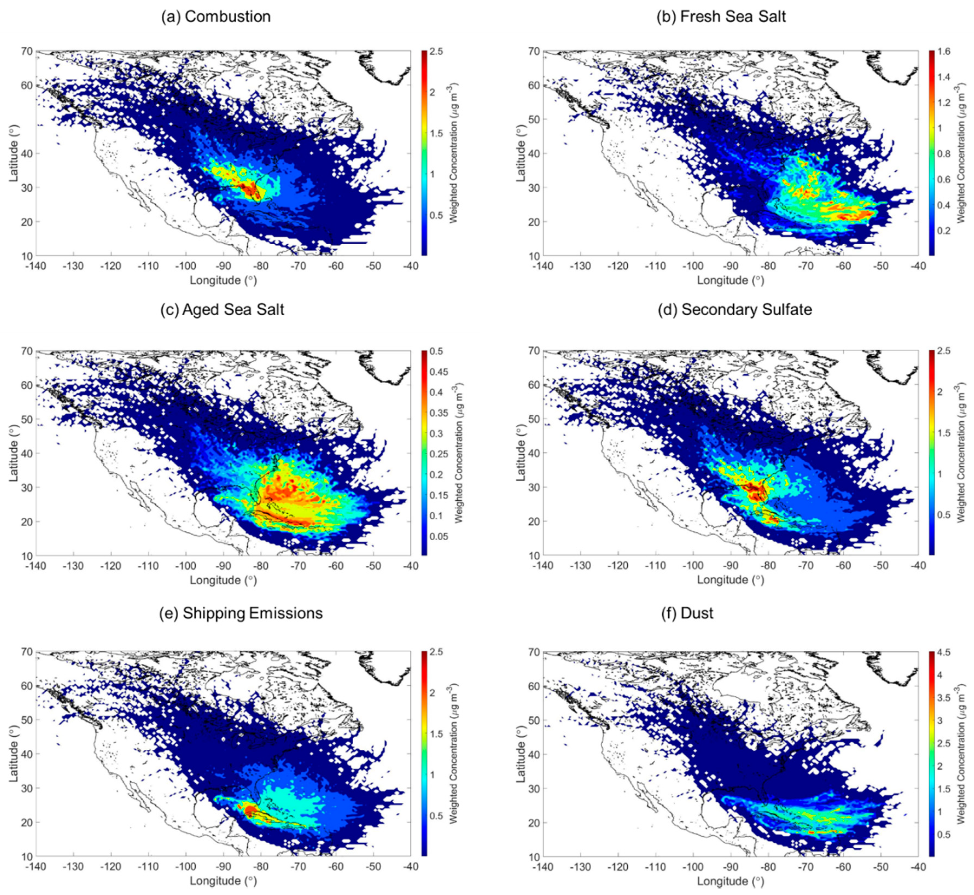
2.4.2. Weight Concentration Weighted Trajectory

A concentration weighted trajectory (CWT) model was used to determine the spatial distribution and transport pathways of potential PM_2.5 sources (e.g., [49]). This approach assigns a weighted concentration to each grid cell obtained by averaging sample concentrations with associated trajectories crossing each grid cell. In order to account for uncertainty, a weighing function was applied to the CWT, which is referred to as weight concentration weighted trajectory (WCWT) [50,51,52]. Weight concentration weighted trajectory maps were developed using the GIS-based software TrajStat [53]. The model used a domain of 160° W to 90° E longitude and 6° N to 90° N latitude with grid cell size 0.5° × 0.5° and incorporated back-trajectories (96 h) from the hybrid single-particle Lagrangian integrated trajectory (HYSPLIT) model [54,55]. Based on previous CWT and potential source contribution function (PSCF) modeling efforts (e.g., [49,52,56,57]), the back trajectories’ ending height was set as 500 m above ground level at Everglades NP. Using the “model vertical velocity” method from the National Centers for Environmental Prediction/National Center for Atmospheric Research (NCEP/NCAR) reanalysis data, trajectories were obtained every 6 h. Seasonal WCWT maps from 2013 to 2018 are provided in Figures S1–S6 of the SI.

3. Results and Discussion

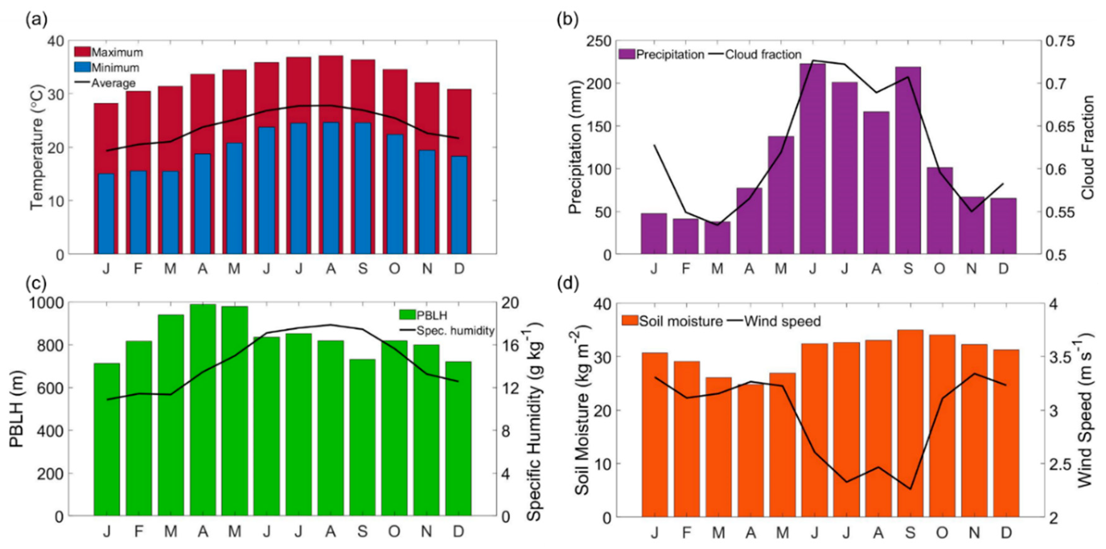
3.1. Meteorological Profile

The section aimed to provide an overview of the meteorological conditions at the studied region (Figure 2). Florida has a subtropical climate with mild winters and hot summers. The summer months extend from June to August (JJA) with little variability in the maximum temperature. The average temperature for the period between 2013 and 2018 was 24.0 ± 3.7 °C with a maximum temperature reported in August of 37.1 ± 2.0 °C (Figure 2a). Minimum temperatures during January, February, and March remained at 15.4 ± 4.1 °C (Figure 2a). Precipitation occurred throughout the year, but primarily between May and October (Figure 2b). Maximum precipitation values were recorded in June (223 ± 71 mm), with the minimum value registered in March (38 ± 71 mm). Higher cloud fractions followed the same trend as the monthly precipitation profile and presented a maximum value in June (0.7 ± 0.07; Figure 2b). Specific humidity values increased in conjunction with the precipitation, with the maximum value recorded in August (17.8 ± 0.48 g kg⁻¹; Figure 2c). Low variability was observed in the PBLH profile throughout the year with a peak during April (989 ± 59 m), a minimum in December (711 ± 63 m), and an annual mean of 823 ± 92 m (Figure 2c). Low monthly variability in soil moisture may be related to precipitation occurring throughout the year (Figure 2d) and the fact that the site is located over a shallow aquifer [58]. The average soil moisture was 30.7 ± 3.67 kg m⁻² for the studied period. Wind speed exhibited higher values during the months with the lowest precipitation, with a mean annual value of 2.95 ± 1.1 m s⁻¹ (Figure 2d). The likelihood of enhanced local dust emissions during periods of higher winds is reduced owing to appreciable soil moisture; this contrasts to drier areas like Central California where there are enhanced dust emissions due to the combination of low soil moisture and increases in wind speed [9].

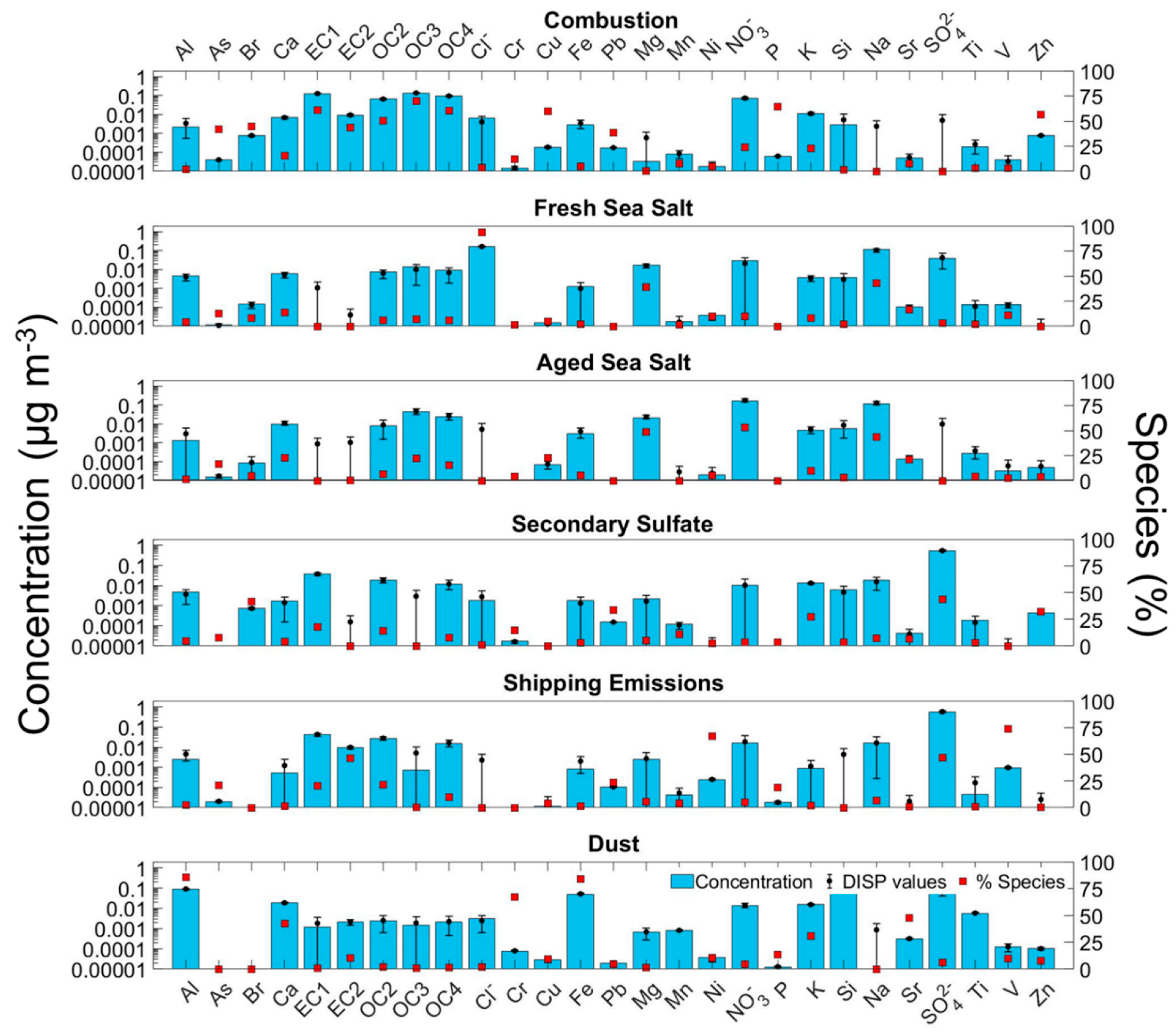
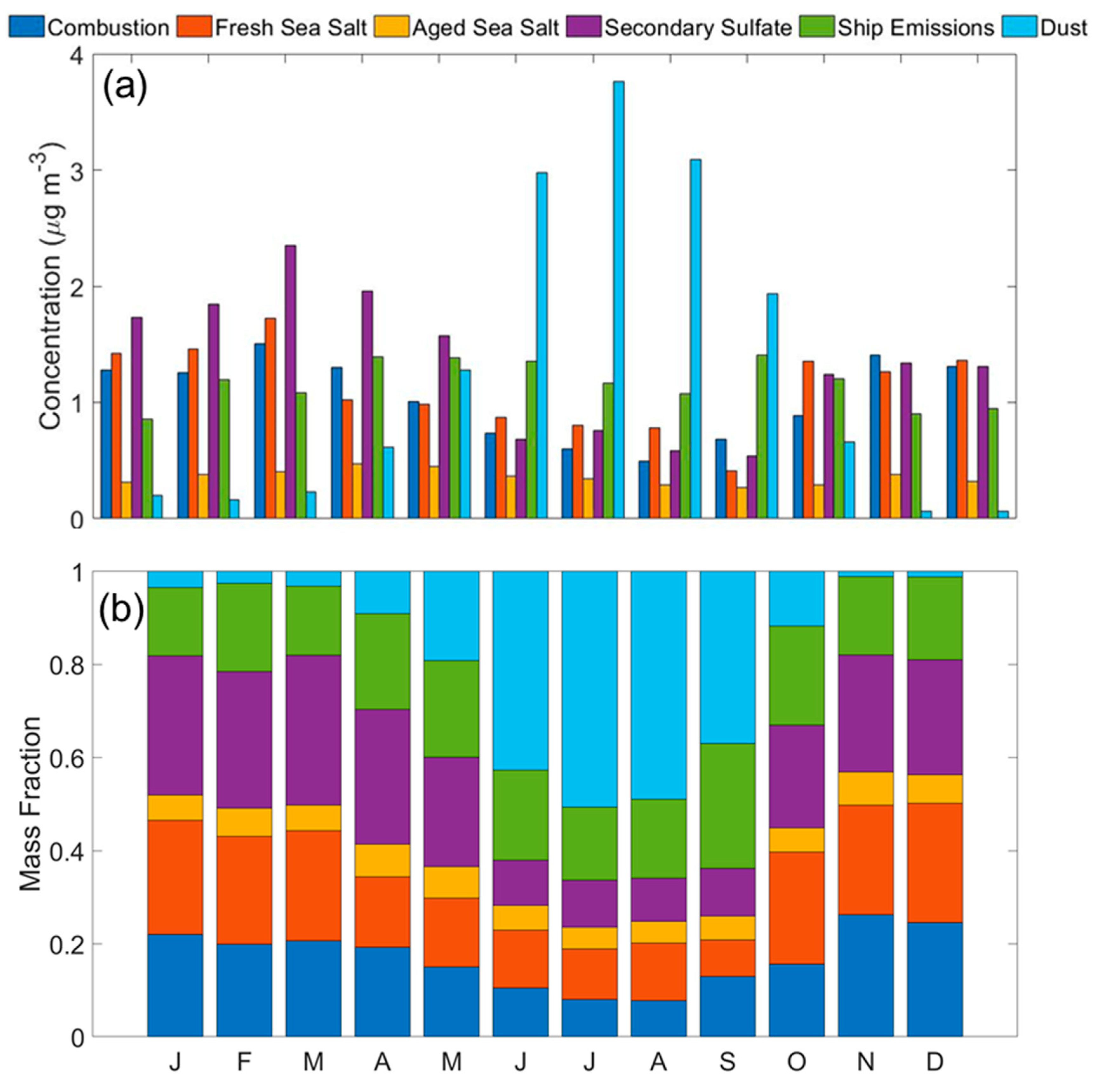
3.2. Sources of PM_2.5

A PMF model based on the elemental and inorganic ion data was used to identify potential emission sources impacting the study area. Several solutions were evaluated to converge on the final solution that has six sources, defined as follows based on their chemical characteristics: (i) combustion; (ii) fresh sea salt; (iii) aged sea salt; (iv) secondary sulfate; (v) shipping emissions; and (vi) dust. The mass concentration of different species and the percent of their mass accounted for by a specific source are shown in Figure 3. The optimal solution was chosen considering the most meaningful physical results, the lowest Q_robust, the Q_true/Q_expected ratio closest to 1, and DISP swap values equal to zero. The concentration and percent of species profiles for the preliminary PMF solutions not used as the final solution are shown in Figures S7–S10. The summary of the PMF model solutions and associated statistics are shown in Tables S5–S6. A mean annual WCWT map is shown in Figure 4 for each of the six factors identified with the PMF model. The results and discussion are included in the sections below.

3.2.1. Combustion

The first factor, defined as combustion, was identified as having influence from biomass burning, vehicle emissions, industrial activities, and fuel/oil sources. Combustion accounts for 17.0% of the total PM_2.5. Dominant constituents influenced by this source factor include the following, with percent values being the fraction of that constituent accounted for by this source: OC3 (69.7%), P (64.4%), EC1 (60.9%), OC4 (60.2%), Cu (59.6%), Zn (56.7%), OC2 (50.5%), Br (44.9%), EC2 (43.6%), As (41.8%), Pb (38.7%), NO₃⁻ (23.7%), and K (22.5%). There were more minor contributions from this source to Ca (15.4%), Cr (12.3%), Sr (7.7%), Mn (7.5%), Ni (4.8%), Fe (4.6%), Cl (3.7%), V (3.1%), Ti (3.0%), Al (2.1%), Si (1.4%), and Mg (0.1%).

Biomass burning has been shown in past work to be an especially large contributor to EC1, P, OC2, OC3, and OC4 [59], which are prominent in this source factor. Combustion associated with either gasoline, diesel, and oil can be traced to concentrations of the OC and EC fractions and various other tracer species [60]. For example, high concentrations of OC3 and OC4 are linked to gasoline emissions as the primary source of combustion, while diesel emissions are characterized by high contributions of EC1. Oil combustion is characterized by enhanced contributions from V, and Ni [60,61]. Residual oil and pulverized coal combustion tracers include As, Cu, and NO₃⁻ [62], while motor oil additives also include Zn and Ca [63]. Zinc and Cu are prominent species in the combustion source factor and have been shown to be pronounced in vehicular emissions [64]. Incinerating activities located in the counties surrounding the sampling site [65] likely contributed to OC1, OC4, EC1, K, Pb, Si, and Zn [66].

The combustion factor’s monthly profile (Figure 5a) shows higher concentrations from October to May (0.89–1.51 µg m⁻³). The relative contribution remained relatively stable throughout the year with an average value of 0.18 ± 0.06 (Figure 5b). As emissions associated with vehicular traffic, industrial activity, and fuel/oil combustion do not necessarily exhibit strong seasonal changes, other factors can explain the monthly profile. For example, the period between October and May features reduced precipitation values and thus less aerosol removal. In addition, those months coincide with the official sugarcane preharvesting burning season (mid-late October to late March) [27] and natural fires during the dry season (April and May) [67]. The WCWT map in Figure 4a shows that the major sources of combustion were over the Florida panhandle and its coast, with additional contributions from fires in the neighboring states [68,69,70]. Seasonal WCWT maps show higher concentrations over the Florida panhandle during SON, DJF, and MAM (Figure S1), in accordance with agricultural and natural fires reported during these months. Interestingly, the WCWT maps revealed that the influence of long-range transport of combustion emissions from fires in areas such as Mexico [15], especially the Yucatan [16], and parts of Central America [71] were not influential relative to local and regional sources.

3.2.2. Fresh and Aged Sea Salt

The fresh and aged sea salt factors represent 12.6% and 6.6% of the total PM_2.5, respectively. The fresh sea salt factor was characterized by the high contribution to Cl⁻ (93.5%), Na (43.1%), and Mg (39.3%). The main differentiating characteristic between the fresh sea salt and the aged sea salt factor was the replacement of Cl⁻ by NO₃⁻ owing to sea salt’s chemical reactivity with acids [72,73]. More specifically, the aged sea salt factor contributed 43.5% to Na, 48.8% to Mg, 53.1% to NO₃⁻, and 0% to Cl⁻. Chloride depletion occurs due to the reaction between sodium chloride (NaCl) and acids such as sulfuric and nitric acids (H₂SO₄ and HNO₃) to form sodium nitrate (NaNO₃) and sodium sulfate (Na₂SO₄) [74,75,76,77], respectively; furthermore, organic acids can participate in depletion reactions as well [78,79,80,81,82]. Size-resolved measurements in other coastal regions have pointed to the abundance of NO₃^– in the supermicrometer size range in contrast to SO₄²⁻ [83,84,85].

The monthly profile (Figure 5a) for fresh sea salt shows higher values between October and March (1.26–1.72 µg m⁻³) with a peak during March revealing a higher contribution (0.30) when compared to the rest of the year (Figure 5b). As sea salt is removed efficiently via wet scavenging with a sharp vertical gradient decreasing with altitude (e.g., [86,87]), the decrease in fresh sea salt expectedly coincides with the enhancement in precipitation between April and September as was also seen for the previously discussed combustion factor. The fresh sea salt WCWT analysis highlights higher mass concentrations associated with trajectories from the east and over the Atlantic Ocean (Figure 4b). The aged sea salt monthly profile was relatively more stable throughout the year (0.36 ± 0.06 µg m⁻³), with slightly higher levels between March–May (0.40–0.47 µg m⁻³). This coincides with the months exhibiting the highest cumulative mass concentrations from three PMF source factors known to emit acids, including combustion, shipping emissions, and secondary SO₄²⁻. In contrast to the fresh sea salt, aged sea salt concentrations were located closer to the coast of Florida and over the Caribbean Sea (Figure 4c), which, as will be shown, was similar to maps for shipping emissions and secondary SO₄²⁻. No apparent seasonal difference was observed for the fresh sea salt WCWT maps (Figure S2), while the seasonal aged sea salt WCWT maps (Figure S3) show a higher concentration during SON over the Atlantic Ocean north off the coast of Florida.

3.2.3. Secondary Sulfate

The next factor, identified as secondary SO₄²⁻, was the dominant factor accounting for 23.0% of the total PM_2.5. This factor contributed the most to SO₄²⁻ (43.6%), which is secondarily produced via gas-to-particle conversion processes from its main precursor SO₂; however, this factor includes other important species that can be secondarily produced as well, such as secondary organic aerosol (SOA) represented by OC2 (14.2%). This factor also included contributions to Br (41.8%), Pb (33.6%), Zn (32.3%), K (27.0%), EC1 (17.9%), Cr (14.6%), Mn (10.9%), As (7.7%), OC4 (7.5%), Na (7.1%), Sr (6.4%), Mg (4.9%), Al (4.4%), Ca (4.0%), P (3.7%), NO₃⁻ (3.4%), Si (3.3%), Ti (2.9%), Fe (2.9%), Ni (2.4%), and Cl (1.0%). As SO₄²⁻ was most pronounced in this factor, it is worth noting that it can be secondarily produced from ocean emissions of dimethylsulfide (DMS) [88], while also originating from both local/regional sources and long-range transport of anthropogenic pollution. The contribution of the various elements to this factor is suggestive of their coemissions with SO₂. For instance, Pb and Zn are coemitted with SO₄²⁻ precursors from municipal solid waste incinerators [89] located 80 km northeast of the sampling site [65]. Other sources coemitting elements along with SO₄²⁻ precursors include: emissions from gasoline vehicles (e.g., Br, EC1, and OC2) [90,91]; Cr electroplater and anodizer facilities (e.g., Cr) [65,92]; and sugarcane preharvest burning (e.g., K, EC1, Zn, and Br) [27,56,93].

The monthly profile and fractional contribution of secondary SO₄²⁻ (Figure 5a,b) follow the same trend as most other factors discussed already, with higher values between October and May (1.24–2.35 µg m⁻³), coincident with reduced precipitation scavenging. Secondary SO₄²⁻ relies on production via aqueous-phase chemistry (e.g., [94]), which benefits in the study region from fairly high year-round values of cloud fraction and humidity (Figure 2). The WCWT spatial results for secondary SO₄²⁻ show more considerable influence from marine regions as compared to the combustion factor (Figure 4d). The same can be observed in the seasonal WCWT maps, where the hotspots were concentrated in the area surrounding the southern coast of Florida. There was not a notable difference in the seasonal WCWT maps for this factor (Figure S4).

3.2.4. Shipping Emissions

The shipping emissions factor represents 20.2% of the total PM_2.5. The high contributions to V (73.7%), Ni (67.1%), SO₄²⁻ (46.9%), EC2 (46.4%), Pb (23.4%), OC2 (21.6%), As (21.3%), EC1 (20.5%), P (18.8%), and OC4 (9.9%) confirmed the primary source of this factor as they are commonly found in low-cost residual oil used as ship fuel [95,96,97,98,99]. The identity of this source was further confirmed by the calculated V:Ni ratio of 3.9, which fits in the range (2.5–5) suggested by Pandolfi et al. [100] as a marker for shipping emissions.

The PM_2.5 monthly profile and fractional contribution for shipping emissions in Figure 5a,b exhibited a bimodal distribution with peaks in April-June (1.35–1.39 µg m⁻³) and September-October (1.20–1.40 µg m⁻³). Compared to the other five factors, this factor showed the least variability among all the aerosol sources. The shipping emissions WCWT map (Figure 4e) shows that substantial contributions come expectedly from marine areas, especially along the Florida, Cuba, Haiti, and the Dominican Republic coasts. Areas of high ship density coincide with high concentrations in the WCWT map. Seasonal WCWT maps do not show notable differences (Figure S5).

3.2.5. Dust

The dust source factor constitutes 20.6% of the total PM_2.5. The high contribution of this source factor to crustal elements like Si (90.5%), Ti (86.9%), Al (85.5%), Fe (83.9%), Mn (75.9%), Cr (67.3%), Sr (47.5%), Ca (42.4%), and K (31.0%) clearly defined this factor as dust [14,32,101,102]. Additional support for this source being linked to dust was the high concentrations and fractional contribution observed during JJA, ranging from 2.98 to 3.76 µg m⁻³ and 0.51 to 0.65, respectively (Figure 5a,b), which is when long-range transport of dust commonly occurs from Africa towards the Caribbean region (e.g., [101,103,104]) and Miami [105,106,107]. It should be noted that these values are lower compared to the long-term means reported in previous studies [108], owing largely to their inclusion of particles with diameters above 2.5 µm [109,110]. The influence of local dust is likely low as the highest dust concentrations coincided with the months with the highest precipitation and soil moisture (Figure 2b,d).

The summer dust WCWT map (Figure 4f) confirmed long-range transport of dust from Northern Africa with the highest concentration observed during this season (Figure S6), consistent with previous studies [14,105,108,111,112,113]. The seasonal WCWT map (Figure S6) shows a clear seasonal difference both in the trajectory paths and in absolute dust concentrations. The summertime (JJA) results show the highest concentrations approaching from the east (Northern Africa).

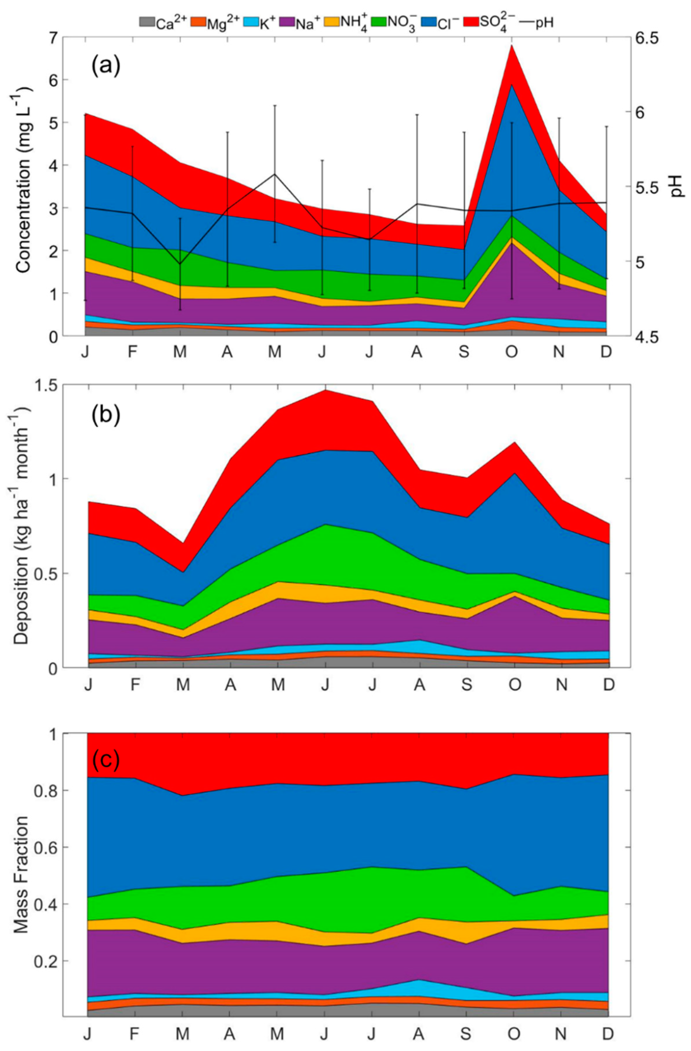
3.3. Precipiation Chemistry Profile

3.3.1. Monthly Profile

The monthly averaged profiles for speciated precipitation data (concentration, deposition flux, and mass fraction) are shown in Figure 6. Wet deposition pH is of great importance in terms of the negative impacts of acid rain. A threshold value of 5.6 is often used to distinguish acid rain (pH < 5.6), symbolic of deionized water in equilibrium with CO₂ (e.g., [114]). However, wet deposition samples contain influence from the original CCN/IN and other gases and aerosols that were scavenged and thus were never pure water. The mean annual pH was 5.32 ± 0.51. Monthly averaged pH values ranged from as low as 4.98 ± 0.31 during March to as high as 5.58 ± 0.46 in May. For contrast, the mean pH was 5.05 at Everglades NP between September 1992 and October 1993 [115]. Documented values for other regions include the following with the caveat that time periods of analysis varied: 5.33–5.51 in Central California [9], 4.20–7.39 in India [116], 4.22–5.68 in Southeastern Brazil [117], 3.52–6.28 in South China [118], 5.71–7.11 in the Southeast Tibetan Plateau [119], and 3.8–6.8 in Eastern France [120]. Regions with the highest reported pH values typically were characterized by having high dust influence and thus carbonate bases such as CaCO₃ ([10]), including in Southwestern Iran (up to 7.38) [121] and Northwestern Iran (up to 8.6) [122], and the Central Himalayas (up to 6.50) [123]. In this work, the wet deposition pH did not exhibit a pH peak during the months with most dust influence in the summer. This was an intriguing result suggestive of transported dust not being a factor in promoting higher pH values in the region’s rainfall.

The total concentration sum of the eight speciated ions was elevated between October and April (Figure 6a), coinciding with the months experiencing the least rain and highest concentrations of most PMF aerosol source factors except shipping emissions and dust. Summer months (JJA) associated with high levels of dust did not show high concentrations of crustal species like Ca²⁺ and Mg²⁺, as observed in the IMPROVE data. This again highlights that the summertime dust season does not play a major role in impacting wet deposition chemistry on a volume-weighted basis. In contrast to their relatively low influence in PM_2.5, sea salt constituents (i.e., Cl⁻ and Na⁺) exhibited the highest concentrations of all ions studied. Sea salt particles are an important source of CCN due to their large size and hygroscopicity, which allows for easier droplet activation as compared to other aerosol types [9,124,125,126]. Higher concentrations of Cl⁻, SO₄²⁻, and Na⁺ in precipitation as compared to PM_2.5 may be partly explained by how the wet deposition data include influence from particles of any size participating in cloud processes or subcloud scavenging. In contrast, the aerosol data were limited to ≤2.5 µm. Sea salt typically ranges from 0.01 and 10 µm [127], with the majority of the mass accounted for by those particles with diameters above 2.5 µm.

An interesting result was the unusually high October levels of Cl⁻ and Na⁺ since sea salt is not expected to show such an increase in a particular month. We also examined the available data back to 1980 and did not observe unusual concentrations as the ones observed during this period. Further analysis of the dataset (2013–2018) showed elevated Cl⁻ and Na⁺ in mid-October 2015 and 2016 (Cl⁻: 4.3–16.1 mg L⁻¹ vs. 0.6–2.2 mg L⁻¹ for other periods; Na⁺: 2.5–9.3 mg L⁻¹ vs. 0.4–1.3 mg L⁻¹ for other periods; Table S7). Even though the concentrations were significantly higher during these few samples (5 out of 14 total for October), the Cl⁻:Na⁺ ratio for these samples (1.70–1.97) was still close to that of pure seawater (Table S7). While a few periods of stronger sea salt emissions may have been likely, another possibility is inspired by previous studies have reported that biomass burning could be an important source of Na⁺ and Cl⁻ (e.g., [128,129,130,131,132]). This has been discussed already to be an important contributor to the regional aerosol pollution between October and March. To probe deeper, images from the Navy Aerosol Analysis and Prediction System (NAAPS; description in Section S1 of SI) were used to detect the possible presence of smoke during the days with high Na⁺ and Cl⁻ concentrations (Figures S10–S16). The NAAPS images did show evidence of smoke for the five week-long periods corresponding to the high Cl⁻ and Na⁺ data points; however, aerosol concentrations of the biomass burning marker K and PMF combustion factor did not show any remarkable enhancement during the time of the five NADP samples of interest (Table S7). Future research can investigate as to whether emissions of Cl⁻ and Na⁺ from regional combustion sources reside in sizes exceeding 2.5 µm, especially during smoke periods, which can help reconcile the difference between the aerosol and wet deposition results for October.

In comparison to the precipitation ion concentrations, the opposite monthly trend was observed for the average monthly deposition fluxes, where higher values were observed during the high precipitation months (April–October; Figure 6b). The highest deposition flux value (1.05 ± 0.26 kg ha⁻¹ month⁻¹) was observed during June when precipitation reached its maximum value. The highest mean annual deposition fluxes were attributed to Cl⁻ (0.53 kg ha⁻¹ month⁻¹), NO₃⁻ (0.32 kg ha⁻¹ month⁻¹), SO₄²⁻ (0.32 kg ha⁻¹ month⁻¹), and Na⁺ (0.30 kg ha⁻¹ month⁻¹). On the other hand, Ca²⁺, K⁺, and Mg²⁺ showed lower deposition fluxes, each being less than 0.1 kg ha⁻¹ month⁻¹. However, deposition fluxes for all three of those ions showed an increase during the summer months compared to other times of the year due most likely to dust influence.

While there were seasonal differences in the concentrations and deposition fluxes of the eight ions, their relative amounts are of significance to gain insight about the relative influence of various sources rather than absolute amounts of constituents. The monthly mass fraction profile was dominated by Cl⁻ (0.27−0.43) and followed by Na⁺ (0.15−0.24), NO₃⁻ (0.08–0.23), and SO₄²⁻ (0.14–0.22; Figure 6c). As observed for other coastal sites, the proximity of the sampling station to the coast explains the high relative contribution of sea salt species like Cl⁻ and Na⁺ (e.g., [133,134]). Grimshaw and Dolske [115] reported decades earlier for the same study region that, based on calculations involving Na ratios, 34% of cations and 65% of anions in wet deposition were of oceanic origin. Sea salt constituents peaked in their mass fractions between October and February.

Chloride-to-sodium ratios are commonly used as a marker for the presence of sea salt and possible Cl⁻ depletion [135,136]. Marine aerosols over the ocean have a Cl⁻:Na⁺ mass concentration ratio for seawater of 1.8 [136,137]. The ratio values for precipitation samples should be carefully interpreted, as uncertainties may arise from this calculation (e.g., [138,139]). For instance, HCl produced after Cl⁻ depletion of sea salt has a longer atmospheric lifetime versus deposition in contrast to its parent aerosol [140]. Little variability was observed between the monthly mass concentration ratios of Cl⁻:Na⁺, with values ranging from 1.74 to 1.84. These results were supportive of a lack of significant sea salt reactivity with inorganic and organic acids [82], which would reduce the ratio. This result was consistent with the PMF analysis showing that fresh sea salt was nearly twice as abundant as aged sea salt. Furthermore, the ratios did not significantly exceed 1.8, pointing to reduced influence from non-salt sources of Cl⁻, such as from coal fired generating facilities and waste incineration, in contrast to wet deposition data from New York [141]. Strong deviations below a ratio of 1.8 could be linked to non-salt sources of Na⁺, such as soil, but that was not the case in this study, consistent with a general lack of influence from crustal species compared to sea salt. Junge and Werby [142] reported on the variability of Cl⁻:Na⁺ mass concentration ratios between the coast and inland U.S. between 1955 and 1956. Ratio values along the coast were lower than those for seawater, ranging from 1.06 to 1.75. However, Cl⁻:Na⁺ ratios drastically dropped farther inland as an indication of enhanced Na⁺ from contributions of non-salt sources (mineral dust). Therefore, it is an important result that the sea salt impacting precipitation was relatively pristine when considering the various other sources impacting the area.

High mass fractions for SO₄²⁻ and NO₃⁻ are suggestive of contributions from anthropogenic emissions and combustion of oil products (e.g., shipping traffic) [143] due to the proximity of urban areas and marine ports (e.g., Miami and Port Everglades). Interestingly, SO₄²⁻ mass fractions were highest between March-April and September (0.20–0.22), whereas NO₃⁻ fractions were highest in June–July (0.21–0.23). Additional contributions to the SO₄²⁻ mass fraction may be attributed to sea salt and secondary production from DMS emissions over the ocean. Additionally, another species commonly linked to SO₄²⁻ and NO₃⁻ anions owing to secondary salt formation is NH₄⁺. Ammonium showed a monthly profile (range = 0.03–0.08) more accordant with SO₄²⁻, suggestive of potential secondary salt formation between those two species (e.g., ammonium sulfate/bisulfate). Mass size distributions of NO₃⁻ commonly indicate significant contributions to the coarse aerosol fraction. Thus, its different monthly profile may be linked to a summertime association with coarse dust, unlike secondarily produced salts.

The least abundant species (Ca²⁺, Mg²⁺, and K⁺) had mass fractions ranging from 0.01 to 0.06 throughout the year. All three species peaked at different times of the year, pointing to different influential sources. For instance, Ca²⁺ peaks in July-August (0.05) and is thus temporally coincident with the dust season, whereas Mg²⁺ peaks between October and February (0.03), which overlaps with when the sea salt constituent mass fractions peak. Lastly, K⁺ peaked in August and September (0.05–0.06), which was likely linked to dust.

3.3.2. Interrelationships

Another way to examine the precipitation chemistry data is to understand the relationship between the species present in precipitation.

Table 1. Correlation coefficient (r) matrix between concentrations of different species in wet deposition samples (NADP). Values shown are statistically significant at the 95% confidence level.

Species	pH	Ca2+	Mg2+	K+	Na+	NH4+	NO3−	Cl−	SO42−
pH	1
Ca2+	0.31	1
Mg2+		0.33	1
K+	0.45	0.16	0.35	1
Na+		0.31	0.99	0.26	1
NH4+	0.51	0.48	0.22	0.42	0.18	1
NO3−	0.07	0.89	0.18	0.09	0.16	0.47	1
Cl−		0.29	0.99	0.26	1.00	0.17	0.15	1
SO42−	−0.29	0.41	0.66	0.20	0.66	0.40	0.40	0.64	1

reports on the interrelationships between the NADP species in the form of a correlation matrix showing values of the Pearson’s correlation coefficient (r) significant at the 95% confidence level (i.e., p-value < 0.05). The strength of the relationship can be categorized as follows for the absolute r value: r = 0–0.2: weak; r = 0.21–0.4: moderately weak; r = 0.41–0.6: moderate; r = 0.61–0.8: moderately strong; and r ≥ 0.81: strongly correlated [144]. Interestingly, all the species concentrations in Table 1 exhibited statistically significant correlations between each other (i.e., p-value < 0.05), but a few were notable. Species that were positively correlated with pH included Ca²⁺ (r = 0.31; moderately weak), NO₃⁻ (r = 0.07; weak), NH₄⁺ (r = 0.51; moderate), and K⁺ (r = 0.45; moderate). The three cations were commonly associated with dust and smoke. Precipitation pH showed a moderate weak negative correlation with the acidic species SO₄²⁻ (r = −0.29), consistent with past work in the study region [145]. The lowest precipitation pH value coincided with the highest SO₄²⁻ concentration, reported in March. Even though high concentrations of SO₄²⁻ were recorded throughout the year, it is possible that these do not have a larger impact on the precipitation pH due to the neutralizing effect of NH₄⁺ [115,146] and Ca²⁺ [147].

The strongest correlation among all of the species was between Cl⁻ and both Na⁺ (r = 1.00) and Mg²⁺ (r = 0.99), which is expected from a near-coastal location influenced by sea salt [10,83,148]. The strongest relationship for the crustal tracer Ca²⁺ was with NO₃⁻ (r = 0.89), which suggests partitioning of NO₃⁻ to dust, as shown in previous studies [149,150,151]. A moderate correlation between Ca²⁺ and SO₄²⁻ (r = 0.41) suggests that NO₃⁻ preferentially participates in reactions with coarse particles that serve as CCN/IN, supported by the monthly profile of mass fractions in the NADP data mentioned earlier. However, there could be potentially enhanced uptake of nitric acid (HNO₃) in existing droplets enriched with Ca²⁺ [10,85,152]. In contrast, NO₃⁻ was weakly correlated with sea salt constituents (Na⁺ and Cl⁻; r = 0.15–0.16), which was surprising as many studies associate NO₃⁻ with sea salt aerosols [83,84,85,148]. Since fresh sea salt was more abundant in the study region than aged sea salt, it is possible that there simply was less NO₃⁻ available to those salt particles seeding the regional clouds. Certainly, more size-resolved measurements of particles in the region can help solidify some of the speculated conclusions reached here regarding relationships between NO₃⁻ with both sea salt and dust particles.

3.4. Precipitation and Aerosol Interrelationships

Concentrations of the precipitation species are related to the PMF source factor and aerosol species concentrations. The PMF and aerosol chemistry concentrations were averaged to the time resolution of NADP data to allow for a direct comparison in the form of a correlation matrix (

Table 2. Correlation coefficient (r) matrix between precipitation (NADP) and aerosol (IMPROVE) composition data. Values shown are statistically significant at the 95% confidence level. The first six aerosol parameters are concentrations of PMF source factors, while the final six at the bottom are selected IMPROVE parameters relevant to the discussion in Section 3.4. Coarse particulate matter (PM_coarse) is calculated as particulate matter with a diameter less than or equal to 10 µm (PM₁₀)–particulate matter with a diameter less than or equal to 2.5 µm (PM_2.5).

Aerosol Parameters	Wet Deposition
	Ca2+	Mg2+	K+	Na+	NH4+	NO3−	Cl−	SO42−
Combustion	0.15					0.16		0.14
Fresh Sea Salt		0.32		0.33			0.33	0.30
Aged Sea Salt
Secondary Sulfate			−0.14		0.15			0.23
Shipping Emissions		−0.17		−0.17			−0.17
Dust					−0.16			−0.18
Mg		0.23		0.24			0.24
Na		0.32		0.33			0.33	0.20
NO3−	0.17
Cl−		0.35		0.36			0.35	0.17
PMcoarse	0.18
Fine Soil		−0.18		−0.19	−0.16		−0.19	−0.21

). Notable results are as follows with the caveat that speculated relationships require more detailed measurements in future research as this analysis relies on surface measurements.

First, the major sea salt constituents in wet deposition (Na⁺, Mg²⁺, and Cl⁻) were similarly related to the same species in the aerosol samples and the PMF fresh sea salt factor. These results suggest how a directly emitted marine aerosol type similarly impacts both PM_2.5 and wet deposition at a coastal site and show that the technique used to relate the aerosol and precipitation data offers promise to build on in future studies. Sulfate from NADP samples showed a weak positive correlation with Na⁺ (r = 0.20) and Cl⁻ (r = 0.17) in the aerosol dataset (but not Mg²⁺), which was not surprising as it is an important constituent in natural sea salt. The same sea salt constituents in wet deposition samples interestingly exhibit a weak negative relationship with fine soil in the aerosol dataset. This relationship can likely be related to the seasonal variation of these species. Sodium, Mg²⁺, and Cl⁻ in the precipitation data peak during the fall months (SON), while aerosol fine soil levels peak during the summer months (JJA). The lack of any relationship between the sea salt constituents in the NADP datasets with the aged sea salt factor from PMF analysis implied that the region’s precipitation was more representative of natural sea salt rather than sea salt that had undergone chemical reactions.

Similar to how sea salt components showed a statistically significant correlation (p-value < 0.05) between the two datasets, the same applies to SO₄²⁻ owing to how the secondary SO₄²⁻ source factor exhibited a moderately weak correlation with precipitation SO₄²⁻ (r = 0.23). Precipitation SO₄²⁻ also exhibited moderately weak (r = 0.30) and weak (r = 0.14) correlations with fresh sea salt and combustion PMF factors, respectively. The weak to moderately weak positive correlations for precipitation SO₄²⁻ can be explained by how SO₄²⁻ was present in sea salt, and it was also produced from secondary formation from both biogenic [149,153] and anthropogenic [154,155] precursor emissions. Precipitation NH₄⁺ exhibited a weak positive correlation with only the secondary SO₄²⁻ PMF factor (r = 0.15), consistent with ammonium sulfate formation. Since precipitation NO₃⁻ did not exhibit any correlation with the same species in the IMPROVE dataset, this suggests that its involvement with wet deposition was based on processes unrelated to surface NO₃⁻ formation in PM_2.5, including its association with CCN/IN larger than 2.5 µm [84,85] and also HNO₃ partitioning to cloud and precipitation drops aloft, as has been documented in other works [10,85,152].

There was a weak positive correlation between precipitation Ca²⁺ and both aerosol NO₃⁻ (r = 0.17) and PM_coarse (r = 0.18). It was already suggested by Table 1 that NO₃⁻ preferentially partitions to coarse dust particles (rather than sea salt), and these results support that notion. The lack of a correlation between precipitation Ca²⁺ and either fine soil or the dust PMF factor could be due to the latter two IMPROVE parameters being limited to the PM_2.5 fraction, whereas the dust particles involved with precipitation processes are larger. An interesting hypothesis motivated by Table 2 warranting future research was that the combustion PMF factor was correlated with both precipitation Ca²⁺ and NO₃⁻ partly because soil dust can be entrained in biomass combustion plumes (e.g., [84,156]).

The lack of other relationships in Table 2 between wet deposition species and pH with aerosol constituents points to the complexities of comparing the datasets and in the processes leading to wet deposition. This was further emphasized by how the correlation coefficients in Table 2 do not exceed a value of 0.36. A major difference is that the IMPROVE speciated data are based on PM_2.5. In contrast, larger particles (mainly sea salt) have been shown here to be especially influential in the collected wet deposition samples. Therefore, any species associated with the coarse sea salt that served as the CCN/IN and any species taken up by existing drops (e.g., HNO₃) would not have been similarly observed at the surface IMPROVE monitoring site. As Table 1 showed, sea salt constituents were positively correlated with all the other species in the NADP dataset. Thus, if they were all linked to the coarse sea salt CCN/IN, this would complicate and reduce the correlations reported in Table 2. Although this highlights an important limitation of comparing the two datasets, it importantly highlights the significance of sea salt and the prominence of its associated constituents in the region’s rainfall. Regarding aerosol–cloud interactions, sea salt was shown here to be an important CCN/IN year-round.

4. Conclusions

The analysis of long-term precipitation chemistry and aerosol data from a coastal site in the Southeast U.S. was used to gain insight into emissions sources impacting both PM_2.5 and wet deposition. The two datasets were intercompared to gain insights into aerosol–precipitation relationships. The points below summarize the findings of this study:

• The Southern Florida coastal site was impacted by a diverse source of pollutants. The following six sources were identified in decreasing contribution to total PM_2.5 (percentage contributions): (i) secondary sulfate (23.0%); (ii) dust (20.6%); (iii) shipping emissions (20.2%); (iv) combustion (17.0%); (v) fresh sea salt (12.6%); and (vi) aged sea salt (6.6%).
• Monthly mean precipitation pH ranges from 4.98 ± 0.31 (March) to 5.58 ± 0.51 (May). Values of pH were negatively related to the acidic anion SO₄²⁻, whereas they were positively related to dust presence as based on the crustal tracer species Ca²⁺.
• The highest mean annual wet deposition fluxes were attributed to Cl⁻, NO₃⁻, SO₄²⁻, and Na+ between April and October, coinciding with months experiencing the most precipitation. Although lower in magnitude, enhanced fluxes of Ca²⁺, K⁺, and Mg²⁺ in summertime coincided with the main dust season.
• Fresh sea salt was the dominant component in the region’s precipitation, unlike surface PM_2.5 owing partly to how the sea salt particles seeding precipitation drops likely exceed 2.5 µm. Aged sea salt was shown to be far less influential in the region’s precipitation.
• Even though dust plays a large role in PM_2.5, it was much less influential in volume-weighted wet deposition concentrations and mass fractions as compared to sea salt.
• A weak positive association between precipitation Ca²⁺ and both aerosol NO₃⁻ and PM_coarse was linked to NO₃⁻ preferentially partitioning to coarse dust.
• Statistically significant correlations (p-value < 0.05) between related parameters indicative of dust, sea salt, and SO₄²⁻ in the NADP and IMPROVE datasets demonstrated that the combined use of these long-term datasets could be useful for other regions to indirectly examine aerosol-precipitation interactions.

References

1. Rosenfeld, D.; Sherwood, S.; Wood, R.; Donner, L. Atmospheric science. Climate effects of aerosol-cloud interactions. Science 2014, 343, 379–380. [Google Scholar] [CrossRef] [PubMed]
2. IPCC. Climate change 2013: The physical science basis. In Contribution of Working Group I to the Fifth Assessment Report of the Intergovernmental Panel on Climate Change; Stocker, T.F., Qin, D., Plattner, G.-K., Tignor, M., Allen, S.K., Boschung, J., Nauels, A., Xia, Y., Bex, V., Midgley, P.M., Eds.; Cambridge University Press: Cambridge, UK; New York, NY, USA, 2013; p. 1535. [Google Scholar]
3. National Academies of Sciences, Engineering and Medicine. Thriving on Our Changing Planet: A Decadal Strategy for Earth Observation from Space; The National Academies Press: Washington, DC, USA, 2018. [Google Scholar] [CrossRef]
4. Sorooshian, A.; Anderson, B.; Bauer, S.E.; Braun, R.A.; Cairns, B.; Crosbie, E.; Dadashazar, H.; Diskin, G.; Ferrare, R.; Flagan, R.C.; et al. Aerosol-cloud-meteorology interaction airborne field investigations: Using lessons learned from the U.S. West Coast in the design of ACTIVATE off the U.S. East Coast. Bull. Amer. Meteor. Soc. 2019, 100, 1511–1528. [Google Scholar] [CrossRef] [Green Version]
5. Wood, R.; Mechoso, C.R.; Bretherton, C.S.; Weller, R.A.; Huebert, B.; Straneo, F.; Albrecht, B.A.; Coe, H.; Allen, G.; Vaughan, G.; et al. The VAMOS Ocean-Cloud-Atmosphere-Land Study Regional Experiment (VOCALS-REx): goals, platforms, and field operations. Atmos. Chem. Phys. 2011, 11, 627–654. [Google Scholar] [CrossRef] [Green Version]
6. Sayer, A.M.; Hsu, N.C.; Lee, J.; Kim, W.V.; Burton, S.; Fenn, M.A.; Ferrare, R.A.; Kacenelenbogen, M.; LeBlanc, S.; Pistone, K.; et al. Two decades observing smoke above clouds in the south-eastern Atlantic Ocean: Deep Blue algorithm updates and validation with ORACLES field campaign data. Atmos. Meas. Tech 2019, 12, 3595–3627. [Google Scholar] [CrossRef] [Green Version]
7. Redemann, J.; Wood, R.; Zuidema, P.; Doherty, S.; Luna, B.; LeBlanc, S.; Diamond, M.; Shinozuka, Y.; Gao, L.; Chang, I.; et al. An overview of the ORACLES (ObseRvations of Aerosols above CLouds and their intEractionS) project: aerosol-cloud-radiation interactions in the Southeast Atlantic basin. Atmos. Chem. Phys. 2020, 449. [Google Scholar] [CrossRef]
8. Sorooshian, A.; Corral, A.F.; Braun, R.A.; Cairns, B.; Crosbie, E.; Ferrare, R.; Hair, J.; Kleb, M.M.; Mardi, A.H.; Maring, H.; et al. Atmospheric research over the Western North Atlantic Ocean region and North American East Coast: A review of past work and challenges ahead. J. Geophys. Res. Atmos. 2020, 125, e2019JD031626. [Google Scholar] [CrossRef]
9. Dadashazar, H.; Ma, L.; Sorooshian, A. Sources of pollution and interrelationships between aerosol and precipitation chemistry at a central California site. Sci. Total Environ. 2019, 651, 1776–1787. [Google Scholar] [CrossRef]
10. Sorooshian, A.; Shingler, T.; Harpold, A.; Feagles, C.W.; Meixner, T.; Brooks, P.D. Aerosol and precipitation chemistry in the southwestern United States: spatiotemporal trends and interrelationships. Atmos. Chem. Phys. 2013, 13, 7361–7379. [Google Scholar] [CrossRef] [Green Version]
11. Mora, M.; Braun, R.A.; Shingler, T.; Sorooshian, A. Analysis of remotely sensed and surface data of aerosols and meteorology for the Mexico Megalopolis Area between 2003 and 2015. J. Geophys. Res. Atmos. 2017, 122, 8705–8723. [Google Scholar] [CrossRef] [Green Version]
12. Hardy, K.A.; Akselsson, R.; Nelson, J.W.; Winchester, J.W. Elemental constituents of Miami aerosol as function of particle size. Environ. Sci. Technol. 1976, 10, 176–182. [Google Scholar] [CrossRef]
13. Johansson, T.; Van Grieken, R.; Winchester, J. Marine influences on aerosol composition in the coastal zone. J. Rech. Atmos. 1974, 8, 761–776. [Google Scholar]
14. Prospero, J.M. Long-range transport of mineral dust in the global atmosphere: impact of African dust on the environment of the southeastern United States. Proc. Natl. Acad. Sci. USA 1999, 96, 3396–3403. [Google Scholar] [CrossRef] [PubMed] [Green Version]
15. Kreidenweis, S.M.; Remer, L.A.; Bruintjes, R.; Dubovik, O. Smoke aerosol from biomass burning in Mexico: Hygroscopic smoke optical model. J. Geophys. Res. Atmos. 2001, 106, 4831–4844. [Google Scholar] [CrossRef] [Green Version]
16. Yokelson, R.J.; Crounse, J.D.; DeCarlo, P.F.; Karl, T.; Urbanski, S.; Atlas, E.; Campos, T.; Shinozuka, Y.; Kapustin, V.; Clarke, A.D.; et al. Emissions from biomass burning in the Yucatan. Atmos. Chem. Phys. 2009, 9, 5785–5812. [Google Scholar] [CrossRef] [Green Version]
17. Medeiros, B.; Nuijens, L. Clouds at Barbados are representative of clouds across the trade wind regions in observations and climate models. Proc. Natl. Acad. Sci. USA 2016, 113, E3062–E3070. [Google Scholar] [CrossRef] [Green Version]
18. Delgadillo, R.; Voss, K.J.; Zuidema, P. Characteristics of optically thin coastal Florida cumuli derived from surface-based lidar measurements. J. Geophys. Res. Atmos. 2018, 123, 10591–10605. [Google Scholar] [CrossRef]
19. Court, A.; Griffiths, J. Thunderstorm climatology. In Thunderstorm Morphology and Dynamics, 2nd ed.; University of Oklahoma Press: Norman, OK, USA, 1986; pp. 9–40. [Google Scholar]
20. Byers, H.R.; Rodebush, H.R. Causes of thunderstorms of the Florida peninsula. J. Meteorol. 1948, 5, 275–280. [Google Scholar] [CrossRef] [Green Version]
21. Prospero, J.M.; Landing, W.M.; Schulz, M. African dust deposition to Florida: Temporal and spatial variability and comparisons to models. J. Geophys. Res. Atmos. 2010, 115. [Google Scholar] [CrossRef] [Green Version]
22. Pollman, C.; Gill, G.; Landing, W.; Guentzel, J.; Bare, D.; Porcella, D.; Zillioux, E.; Atkeson, T. Overview of the Florida atmospheric mercury study (Fams). Water Air Soil Pollut. 1995, 80, 285–290. [Google Scholar] [CrossRef]
23. U.S. Census Bureau. QuickFacts Miami-Dade County, Florida; United States. 2018. Available online: https://www.census.gov/quickfacts/miamidadecountyflorida (accessed on 1 May 2020).
24. Glaser, P.H.; Hansen, B.C.; Donovan, J.J.; Givnish, T.J.; Stricker, C.A.; Volin, J.C. Holocene dynamics of the Florida Everglades with respect to climate, dustfall, and tropical storms. Proc. Natl. Acad. Sci. USA 2013, 110, 17211–17216. [Google Scholar] [CrossRef] [Green Version]
25. Ingebritsen, S.; McVoy, C.; Glaz, B.; Park, W. Florida Everglades. Land Subsid. USA Circa 1999, 1182, 95–120. [Google Scholar]
26. USDA-NASS. Florida County Estimates Sugarcane 2017–2018. United States Department of Agriculture National Agricultural Statistics Service Southern Region. 2019. Available online: https://www.nass.usda.gov/Statistics_by_State/Florida/Publications/County_Estimates/2018/FLSugarcane2018.pdf (accessed on 1 May 2020).
27. Sevimoğlu, O.; Rogge, W.F. Seasonal variations of PM10—Trace elements, PAHs and levoglucosan: Rural sugarcane growing area versus coastal urban area in Southeastern Florida, USA. Part II: Elemental concentrations. Particuology 2019, 46, 99–108. [Google Scholar] [CrossRef]
28. Dawson, L.; Boopathy, R. Use of post-harvest sugarcane residue for ethanol production. Bioresour. Technol. 2007, 98, 1695–1699. [Google Scholar] [CrossRef] [PubMed]
29. Frias, M.; Villar-Cocina, E.; Valencia-Morales, E. Characterisation of sugar cane straw waste as pozzolanic material for construction: calcining temperature and kinetic parameters. Waste Manag. 2007, 27, 533–538. [Google Scholar] [CrossRef]
30. Silva, F.S.; Cristale, J.; Andre, P.A.; Saldiva, P.H.N.; Marchi, M.R.R. PM2.5 and PM10: The influence of sugarcane burning on potential cancer risk. Atmos. Environ. 2010, 44, 5133–5138. [Google Scholar] [CrossRef]
31. Sevimoglu, O.; Rogge, W.F. Seasonal size-segregated PM10 and PAH concentrations in a rural area of sugarcane agriculture versus a coastal urban area in Southeastern Florida, USA. Particuology 2016, 28, 52–59. [Google Scholar] [CrossRef]
32. Malm, W.C.; Sisler, J.F.; Huffman, D.; Eldred, R.A.; Cahill, T.A. Spatial and seasonal trends in particle concentration and optical extinction in the United States. J. Geophys. Res. Atmos. 1994, 99, 1347–1370. [Google Scholar] [CrossRef]
33. National Atmospheric Deposition Program (NADP). Available online: http://nadp.slh.wisc.edu/ntn/ (accessed on 1 May 2020).
34. The Interagency Monitoring of Protected Visual Environments (IMPROVE). Available online: http://views.cira.colostate.edu/fed/QueryWizard/Default.aspx (accessed on 1 May 2020).
35. Chow, J.C.; Watson, J.G.; Chen, L.W.; Chang, M.C.; Robinson, N.F.; Trimble, D.; Kohl, S. The IMPROVE_A temperature protocol for thermal/optical carbon analysis: maintaining consistency with a long-term database. J. Air Waste Manag. Assoc. 2007, 57, 1014–1023. [Google Scholar] [CrossRef] [Green Version]
36. Chow, J.C.; Watson, J.G.; Pritchett, L.C.; Pierson, W.R.; Frazier, C.A.; Purcell, R.G. The dri thermal/optical reflectance carbon analysis system: Description, evaluation and applications in U.S. Air quality studies. Atmos. Environ. Part A Gen. Top. 1993, 27, 1185–1201. [Google Scholar] [CrossRef]
37. Lim, S.; Lee, M.; Lee, G.; Kim, S.; Yoon, S.; Kang, K. Ionic and carbonaceous compositions of PM10, PM2.5 and PM1.0 at Gosan ABC Superstation and their ratios as source signature. Atmos. Chem. Phys. 2012, 12, 2007–2024. [Google Scholar] [CrossRef] [Green Version]
38. Chow, J.C.; Lowenthal, D.H.; Chen, L.W.; Wang, X.; Watson, J.G. Mass reconstruction methods for PM2.5: A review. Air Qual. Atmos. Health 2015, 8, 243–263. [Google Scholar] [CrossRef] [PubMed] [Green Version]
39. Solomon, P.A.; Crumpler, D.; Flanagan, J.B.; Jayanty, R.K.; Rickman, E.E.; McDade, C.E. U.S. national PM2.5 Chemical Speciation Monitoring Networks-CSN and IMPROVE: description of networks. J. Air Waste Manag. Assoc. 2014, 64, 1410–1438. [Google Scholar] [CrossRef] [PubMed] [Green Version]
40. USEPA AQS. EPA AirData Air Quality System (AQS) Monitors. Available online: https://epa.maps.arcgis.com/apps/webappviewer/index.html?id=5f239fd3e72f424f98ef3d5def547eb5&extent=-146.2334,13.1913,-46.3896,56.5319 (accessed on 1 May 2020).
41. Randles, C.A.; Da Silva, A.M.; Buchard, V.; Colarco, P.R.; Darmenov, A.; Govindaraju, R.; Smirnov, A.; Holben, B.; Ferrare, R.; Hair, J.; et al. The MERRA-2 aerosol reanalysis, 1980-onward, Part I: System description and data assimilation evaluation. J. Clim. 2017, 30, 6823–6850. [Google Scholar] [CrossRef] [PubMed]
42. Rodell, M.; Houser, P.R.; Jambor, U.; Gottschalck, J.; Mitchell, K.; Meng, C.J.; Arsenault, K.; Cosgrove, B.; Radakovich, J.; Bosilovich, M.; et al. The global land data assimilation system. Bull. Amer. Meteor. Soc. 2004, 85, 381. [Google Scholar] [CrossRef] [Green Version]
43. Acker, J.G.; Leptoukh, G. Online analysis enhances use of NASA earth science data. Eos Trans. 2007, 88, 14–17. [Google Scholar] [CrossRef]
44. Hopke, P.K. Review of receptor modeling methods for source apportionment. J. Air Waste Manag. Assoc. 2016, 66, 237–259. [Google Scholar] [CrossRef]
45. Brown, S.G.; Eberly, S.; Paatero, P.; Norris, G.A. Methods for estimating uncertainty in PMF solutions: examples with ambient air and water quality data and guidance on reporting PMF results. Sci. Total Environ. 2015, 518, 626–635. [Google Scholar] [CrossRef] [Green Version]
46. Reff, A.; Eberly, S.I.; Bhave, P.V. Receptor modeling of ambient particulate matter data using positive matrix factorization: review of existing methods. J. Air Waste Manag. Assoc. 2007, 57, 146–154. [Google Scholar] [CrossRef] [Green Version]
47. Norris, G.; Duvall, R.; Brown, S.; Bai, S. EPA Positive Matrix Factorization (PMF) 5.0 Fundamentals and User Guide. 2014. Available online: https://www.epa.gov/sites/production/files/2015-02/documents/pmf_5.0_user_guide.pdf (accessed on 1 May 2020).
48. Kim, E.; Hopke, P.K.; Edgerton, E.S. Source identification of atlanta aerosol by positive matrix factorization. J. Air Waste Manag. Assoc. 2003, 53, 731–739. [Google Scholar] [CrossRef] [Green Version]
49. Hsu, Y.K.; Holsen, T.M.; Hopke, P.K. Comparison of hybrid receptor models to locate PCB sources in Chicago. Atmos. Environ. 2003, 37, 545–562. [Google Scholar] [CrossRef]
50. Seibert, P.; Kromp-Kolb, H.; Baltensperger, U.; Jost, D.; Schwikowski, M.; Kasper, A.; Puxbaum, H. Trajectory analysis of aerosol measurements at high alpine sites. In Air Pollution Modeling and Its Application X. NATO · Challenges of Modern Society; Gryning, S.E., Millán, M.M., Eds.; Springer: Boston, MA, USA, 1994; Volume 18, pp. 689–693. [Google Scholar]
51. Sun, T.Z.; Che, H.Z.; Qi, B.; Wang, Y.Q.; Dong, Y.S.; Xia, X.G.; Wang, H.; Gui, K.; Zheng, Y.; Zhao, H.J.; et al. Aerosol optical characteristics and their vertical distributions under enhanced haze pollution events: effect of the regional transport of different aerosol types over eastern China. Atmos. Chem. Phys. 2018, 18, 2949–2971. [Google Scholar] [CrossRef] [Green Version]
52. Polissar, A.V.; Hopke, P.K.; Paatero, P.; Kaufmann, Y.J.; Hall, D.K.; Bodhaine, B.A.; Dutton, E.G.; Harris, J.M. The aerosol at Barrow, Alaska: long-term trends and source locations. Atmos. Environ. 1999, 33, 2441–2458. [Google Scholar] [CrossRef]
53. Wang, Y.Q.; Zhang, X.Y.; Draxler, R.R. TrajStat: GIS-based software that uses various trajectory statistical analysis methods to identify potential sources from long-term air pollution measurement data. Environ. Model. Software 2009, 24, 938–939. [Google Scholar] [CrossRef]
54. Stein, A.F.; Draxler, R.R.; Rolph, G.D.; Stunder, B.J.B.; Cohen, M.D.; Ngan, F. NOAA’s HYSPLITt atmospheric transport and dispersion modeling system. Bull. Amer. Meteor. Soc. 2015, 96, 2059–2077. [Google Scholar] [CrossRef]
55. Rolph, G.; Stein, A.; Stunder, B. Real-time Environmental Applications and Display sYstem: READY. Environ. Model. Software 2017, 95, 210–228. [Google Scholar] [CrossRef]
56. Masiol, M.; Hopke, P.K.; Felton, H.D.; Frank, B.P.; Rattigan, O.V.; Wurth, M.J.; LaDuke, G.H. Source apportionment of PM2.5 chemically speciated mass and particle number concentrations in New York City. Atmos. Environ. 2017, 148, 215–229. [Google Scholar] [CrossRef]
57. Xin, J.Y.; Du, W.P.; Wang, Y.S.; Gao, Q.X.; Li, Z.Q.; Wang, M.X. Aerosol optical properties affected by a strong dust Storm over central and northern China. Adv. Atmos. Sci. 2010, 27, 562–574. [Google Scholar] [CrossRef]
58. Zhang, M.J.; Singh, H.V.; Migliaccio, K.W.; Kisekka, I. Evaluating water table response to rainfall events in a shallow aquifer and canal system. Hydrol. Process. 2017, 31, 3907–3919. [Google Scholar] [CrossRef]
59. Schlosser, J.S.; Braun, R.A.; Bradley, T.; Dadashazar, H.; MacDonald, A.B.; Aldhaif, A.A.; Aghdam, M.A.; Mardi, A.H.; Xian, P.; Sorooshian, A. Analysis of aerosol composition data for western United States wildfires between 2005 and 2015: Dust emissions, chloride depletion, and most enhanced aerosol constituents. J. Geophys. Res. Atmos. 2017, 122, 8951–8966. [Google Scholar] [CrossRef] [PubMed]
60. Kim, E.; Hopke, P.K. Source apportionment of fine particles in Washington, DC, utilizing temperature-resolved carbon fractions. J. Air Waste Manag. Assoc. 2004, 54, 773–785. [Google Scholar] [CrossRef] [PubMed]
61. Corbin, J.C.; Mensah, A.A.; Pieber, S.M.; Orasche, J.; Michalke, B.; Zanatta, M.; Czech, H.; Massabo, D.; Buatier de Mongeot, F.; Mennucci, C.; et al. Trace metals in soot and PM2.5 from heavy-fuel-oil combustion in a marine engine. Environ. Sci. Technol. 2018, 52, 6714–6722. [Google Scholar] [CrossRef] [PubMed] [Green Version]
62. Linak, W.P.; Miller, C.A.; Wendt, J.O. Comparison of particle size distributions and elemental partitioning from the combustion of pulverized coal and residual fuel oil. J. Air Waste Manag. Assoc. 2000, 50, 1532–1544. [Google Scholar] [CrossRef] [PubMed] [Green Version]
63. Ålander, T.; Antikainen, E.; Raunemaa, T.; Elonen, E.; Rautiola, A.; Torkkell, K. Particle emissions from a small two-stroke engine: effects of fuel, lubricating oil, and exhaust aftertreatment on particle characteristics. Aerosol Sci. Technol. 2005, 39, 151–161. [Google Scholar] [CrossRef] [Green Version]
64. Pant, P.; Harrison, R.M. Estimation of the contribution of road traffic emissions to particulate matter concentrations from field measurements: A review. Atmos. Environ. 2013, 77, 78–97. [Google Scholar] [CrossRef]
65. DARM. AirInfo Data Search. Florida Department of Environmental Protection Division of Air Resource Management’s. 2013. Available online: https://prodenv.dep.state.fl.us/DarmAircom/public/searchFacilityPILoad.action (accessed on 1 May 2020).
66. Hwang, I.-J.; Hopke, P.K. Comparison of source apportionment of PM 2.5 using PMF2 and EPA PMF version 2. Asian J. Atmos. Environ. 2011, 5, 86–96. [Google Scholar] [CrossRef] [Green Version]
67. Lang, Q.; Zhang, Q.; Jaffe, R. Organic aerosols in the Miami area, USA: temporal variability of atmospheric particles and wet/dry deposition. Chemosphere 2002, 47, 427–441. [Google Scholar] [CrossRef]
68. Liu, X.; Zhang, Y.; Huey, L.; Yokelson, R.; Wang, Y.; Jimenez, J.; Campuzano-Jost, P.; Beyersdorf, A.; Blake, D.; Choi, Y. Agricultural fires in the southeastern US during SEAC4RS: Emissions of trace gases and particles and evolution of ozone, reactive nitrogen, and organic aerosol. J. Geophys. Res. Atmos. 2016, 121, 7383–7414. [Google Scholar] [CrossRef] [Green Version]
69. McCarty, J.L.; Korontzi, S.; Justice, C.O.; Loboda, T. The spatial and temporal distribution of crop residue burning in the contiguous United States. Sci. Total Environ. 2009, 407, 5701–5712. [Google Scholar] [CrossRef]
70. Reid, S.B.; Funk, T.H.; Sullivan, D.C.; Stiefer, P.S.; Arkinson, H.L.; Brown, S.G.; Chinkin, L.R. Research and development of emission inventories for planned burning activities for the Central State Regional Air Planning Association. In Proceedings of the 13th International Emission Inventory Conference, Clearwater, FL, USA, 8–10 June 2004. [Google Scholar]
71. Wang, J.; Christopher, S.A.; Nair, U.S.; Reid, J.S.; Prins, E.M.; Szykman, J.; Hand, J.L. Mesoscale modeling of Central American smoke transport to the United States: 1. “Top-down” assessment of emission strength and diurnal variation impacts. J. Geophys. Res. Atmos. 2006, 111. [Google Scholar] [CrossRef] [Green Version]
72. Kotchenruther, R.A. The effects of marine vessel fuel sulfur regulations on ambient PM2.5 at coastal and near coastal monitoring sites in the U.S. Atmos. Environ. 2017, 151, 52–61. [Google Scholar] [CrossRef]
73. Adachi, K.; Buseck, P.R. Changes in shape and composition of sea-salt particles upon aging in an urban atmosphere. Atmos. Environ. 2015, 100, 1–9. [Google Scholar] [CrossRef]
74. Qin, Y.; Oduyemi, K.; Chan, L.Y. Comparative testing of PMF and CFA models. Chemom. Intellig. Lab. Syst. 2002, 61, 75–87. [Google Scholar] [CrossRef]
75. Seinfeld, J.H.; Pandis, S.N. Atmospheric Chemistry and Physics: From Air Pollution to Climate Change, 3rd ed; John Wiley & Sons, Inc.: Hoboken, NJ, USA, 2016. [Google Scholar]
76. Song, X.-H.; Polissar, A.V.; Hopke, P.K. Sources of fine particle composition in the northeastern US. Atmos. Environ. 2001, 35, 5277–5286. [Google Scholar] [CrossRef]
77. Perez, N.; Pey, J.; Reche, C.; Cortes, J.; Alastuey, A.; Querol, X. Impact of harbour emissions on ambient PM10 and PM2.5 in Barcelona (Spain): Evidences of secondary aerosol formation within the urban area. Sci. Total Environ. 2016, 571, 237–250. [Google Scholar] [CrossRef] [PubMed]
78. Braun, R.A.; Dadashazar, H.; MacDonald, A.B.; Aldhaif, A.M.; Maudlin, L.C.; Crosbie, E.; Aghdam, M.A.; Hossein Mardi, A.; Sorooshian, A. Impact of wildfire emissions on chloride and bromide depletion in marine aerosol particles. Environ. Sci. Technol. 2017, 51, 9013–9021. [Google Scholar] [CrossRef] [PubMed]
79. Kerminen, V.M.; Teinila, K.; Hillamo, R.; Pakkanen, T. Substitution of chloride in sea-salt particles by inorganic and organic anions. J. Aerosol Sci. 1998, 29, 929–942. [Google Scholar] [CrossRef]
80. Virkkula, A.; Teinila, K.; Hillamo, R.; Matti-Kerminen, V.; Saarikoski, S.; Aurela, M.; Koponen, I.K.; Kulmala, M. Chemical size distributions of boundary layer aerosol over the Atlantic Ocean and at an Antarctic site. J. Geophys. Res. Atmos. 2006, 111. [Google Scholar] [CrossRef]
81. Keene, W.C.; Khalil, M.A.K.; Erickson, D.J.; McCulloch, A.; Graedel, T.E.; Lobert, J.M.; Aucott, M.L.; Gong, S.L.; Harper, D.B.; Kleiman, G.; et al. Composite global emissions of reactive chlorine from anthropogenic and natural sources: Reactive chlorine emissions inventory. J. Geophys. Res. Atmos. 1999, 104, 8429–8440. [Google Scholar] [CrossRef] [Green Version]
82. AzadiAghdam, M.; Braun, R.A.; Edwards, E.-L.; Bañaga, P.A.; Cruz, M.T.; Betito, G.; Cambaliza, M.O.; Dadashazar, H.; Lorenzo, G.R.; Ma, L.; et al. On the nature of sea salt aerosol at a coastal megacity: Insights from Manila, Philippines in Southeast Asia. Atmos. Environ. 2019, 216, 116922. [Google Scholar] [CrossRef]
83. Cruz, M.T.; Banaga, P.A.; Betito, G.; Braun, R.A.; Stahl, C.; Aghdam, M.A.; Cambaliza, M.O.; Dadashazar, H.; Hilario, M.R.; Lorenzo, G.R.; et al. Size-resolved composition and morphology of particulate matter during the southwest monsoon in Metro Manila, Philippines. Atmos. Chem. Phys. 2019, 19, 10675–10696. [Google Scholar] [CrossRef] [Green Version]
84. Maudlin, L.; Wang, Z.; Jonsson, H.; Sorooshian, A. Impact of wildfires on size-resolved aerosol composition at a coastal California site. Atmos. Environ. 2015, 119, 59–68. [Google Scholar] [CrossRef] [Green Version]
85. Prabhakar, G.; Ervens, B.; Wang, Z.; Maudlin, L.C.; Coggon, M.M.; Jonsson, H.H.; Seinfeld, J.H.; Sorooshian, A. Sources of nitrate in stratocumulus cloud water: Airborne measurements during the 2011 E-PEACE and 2013 NiCE studies. Atmos. Environ. 2014, 97, 166–173. [Google Scholar] [CrossRef] [Green Version]
86. Murphy, D.M.; Froyd, K.D.; Bian, H.S.; Brock, C.A.; Dibb, J.E.; DiGangi, J.P.; Diskin, G.; Dollner, M.; Kupc, A.; Scheuer, E.M.; et al. The distribution of sea-salt aerosol in the global troposphere. Atmos. Chem. Phys. 2019, 19, 4093–4104. [Google Scholar] [CrossRef] [Green Version]
87. MacDonald, A.B.; Dadashazar, H.; Chuang, P.Y.; Crosbie, E.; Wang, H.; Wang, Z.; Jonsson, H.H.; Flagan, R.C.; Seinfeld, J.H.; Sorooshian, A. Characteristic vertical profiles of cloud water composition in marine stratocumulus clouds and relationships with precipitation. J. Geophys. Res. Atmos. 2018, 123, 3704–3723. [Google Scholar] [CrossRef] [PubMed]
88. Keller, M.D. Dimethyl sulfide production and marine phytoplankton: The importance of species composition and cell size. Biol. Oceanogr. 1989, 6, 375–382. [Google Scholar] [CrossRef]
89. Pacyna, J.M.; Pacyna, E.G. An assessment of global and regional emissions of trace metals to the atmosphere from anthropogenic sources worldwide. Environ. Rev. 2001, 9, 269–298. [Google Scholar] [CrossRef]
90. Rose, K. Source allocation of columbia gorge IMPROVE data with positive matrix factorization. Appendix E of Chemical Concentration Balance Source Apportionment of PM2.5 2004. Available online: http://citeseerx.ist.psu.edu/viewdoc/download?doi=10.1.1.424.7044&rep=rep1&type=pdf (accessed on 1 May 2020).
91. Kim, E.; Hopke, P.K. Improving source apportionment of fine particles in the eastern United States utilizing temperature-resolved carbon fractions. J. Air Waste Manag. Assoc. 2005, 55, 1456–1463. [Google Scholar] [CrossRef] [PubMed] [Green Version]
92. Brown, R.J.C.; Van Aswegen, S.; Webb, W.R.; Goddard, S.L. UK concentrations of chromium and chromium (VI), measured as water soluble chromium, in PM10. Atmos. Environ. 2014, 99, 385–391. [Google Scholar] [CrossRef]
93. Urban, R.C.; Lima-Souza, M.; Caetano-Silva, L.; Queiroz, M.E.C.; Nogueira, R.F.P.; Allen, A.G.; Cardoso, A.A.; Held, G.; Campos, M.L.A.M. Use of levoglucosan, potassium, and water-soluble organic carbon to characterize the origins of biomass-burning aerosols. Atmos. Environ. 2012, 61, 562–569. [Google Scholar] [CrossRef]
94. Barth, M.C.; Rasch, P.J.; Kiehl, J.T.; Benkovitz, C.M.; Schwartz, S.E. Sulfur chemistry in the National Center for Atmospheric Research Community Climate Model: Description, evaluation, features, and sensitivity to aqueous chemistry. J. Geophys. Res. Atmos. 2000, 105, 1387–1415. [Google Scholar] [CrossRef]
95. Karanasiou, A.A.; Siskos, P.A.; Eleftheriadis, K. Assessment of source apportionment by Positive Matrix Factorization analysis on fine and coarse urban aerosol size fractions. Atmos. Environ. 2009, 43, 3385–3395. [Google Scholar] [CrossRef]
96. Viana, M.; Amato, F.; Alastuey, A.; Querol, X.; Moreno, T.; Dos Santos, S.G.; Herce, M.D.; Fernandez-Patier, R. Chemical tracers of particulate emissions from commercial shipping. Environ. Sci. Technol. 2009, 43, 7472–7477. [Google Scholar] [CrossRef] [PubMed]
97. Viana, M.; Kuhlbusch, T.A.J.; Querol, X.; Alastuey, A.; Harrison, R.M.; Hopke, P.K.; Winiwarter, W.; Vallius, A.; Szidat, S.; Prevot, A.S.H.; et al. Source apportionment of particulate matter in Europe: A review of methods and results. J. Aerosol Sci. 2008, 39, 827–849. [Google Scholar] [CrossRef]
98. Hobbs, P.V.; Garrett, T.J.; Ferek, R.J.; Strader, S.R.; Hegg, D.A.; Frick, G.M.; Hoppel, W.A.; Gasparovic, R.F.; Russell, L.M.; Johnson, D.W.; et al. Emissions from ships with respect to their effects on clouds. J. Atmos. Sci. 2000, 57, 2570–2590. [Google Scholar] [CrossRef] [Green Version]
99. Isakson, J.; Persson, T.A.; Selin Lindgren, E. Identification and assessment of ship emissions and their effects in the harbour of Göteborg, Sweden. Atmos. Environ. 2001, 35, 3659–3666. [Google Scholar] [CrossRef]
100. Pandolfi, M.; Gonzalez-Castanedo, Y.; Alastuey, A.; Jesus, D.; Mantilla, E.; De La Campa, A.S.; Querol, X.; Pey, J.; Amato, F.; Moreno, T. Source apportionment of PM 10 and PM 2.5 at multiple sites in the strait of Gibraltar by PMF: impact of shipping emissions. Environ. Sci. Pollut. Res. 2011, 18, 260–269. [Google Scholar] [CrossRef]
101. Perry, K.D.; Cahill, T.A.; Eldred, R.A.; Dutcher, D.D.; Gill, T.E. Long-range transport of North African dust to the eastern United States. J. Geophys. Res. Atmos. 1997, 102, 11225–11238. [Google Scholar] [CrossRef]
102. Flocchini, R.G.; Cahill, T.A.; Pitchford, M.L.; Eldred, R.A.; Feeney, P.J.; Ashbaugh, L.L. Characterization of particles in the arid west. Atmos. Environ. 1981, 15, 2017–2030. [Google Scholar] [CrossRef]
103. Prospero, J.M.; Nees, R.T. Dust concentration in the atmosphere of the equatorial north atlantic: possible relationship to the sahelian drought. Science 1977, 196, 1196–1198. [Google Scholar] [CrossRef] [Green Version]
104. Carlson, T.N.; Prospero, J.M. The large-scale movement of Saharan air outbreaks over the Northern Equatorial Atlantic. J. Appl. Meteorol. Climatol 1972, 11, 283–297. [Google Scholar] [CrossRef]
105. Savoie, D.; Prospero, J. Aerosol concentration statistics for the northern tropical Atlantic. J. Geophys. Res. 1977, 82, 5954–5964. [Google Scholar] [CrossRef]
106. Prospero, J.M. Assessing the impact of advected African dust on air quality and health in the eastern United States. Hum. Ecol. Risk Assess. Int. J. 1999, 5, 471–479. [Google Scholar] [CrossRef]
107. Prospero, J.M. Long-term measurements of the transport of African mineral dust to the southeastern United States: Implications for regional air quality. J. Geophys. Res. Atmos. 1999, 104, 15917–15927. [Google Scholar] [CrossRef] [Green Version]
108. Zuidema, P.; Alvarez, C.; Kramer, S.J.; Custals, L.; Izaguirre, M.; Sealy, P.; Prospero, J.M.; Blades, E. Is Summer African dust arriving earlier to Barbados? The updated long-term in situ dust mass concentration time series from Ragged Point, Barbados, and Miami, Florida. Bull. Amer. Meteor. Soc. 2019, 100, 1981–1986. [Google Scholar] [CrossRef]
109. Kramer, S.J.; Alvarez, C.; Barkley, A.; Colarco, P.R.; Custals, L.; Delgadillo, R.; Gaston, C.; Govindaraju, R.; Zuidema, P. Apparent dust size discrepancy in aerosol reanalysis in north African dust after long-range transport. Atmos. Chem. Phys. Discuss. 2020, 2020, 1–32. [Google Scholar] [CrossRef]
110. Kramer, S.J.; Kirtman, B.P.; Zuidema, P.; Ngan, F. Subseasonal variability of elevated dust concentrations over South Florida. J. Geophys. Res. Atmos. 2020, 125, e2019JD031874. [Google Scholar] [CrossRef]
111. Prospero, J.M.; Bonatti, E.; Schubert, C.; Carlson, T.N. Dust in the Caribbean atmosphere traced to an African dust storm. Earth Planet. Sci. Lett. 1970, 9, 287–293. [Google Scholar] [CrossRef]
112. Aldhaif, A.M.; Lopez, D.H.; Dadashazar, H.; Sorooshian, A. Sources, frequency, and chemical nature of dust events impacting the United States East Coast. Atmos. Environ. 2020, 231, 117456. [Google Scholar] [CrossRef]
113. Prospero, J.M.; Collard, F.-X.; Molinié, J.; Jeannot, A. Characterizing the annual cycle of African dust transport to the Caribbean Basin and South America and its impact on the environment and air quality. Glob. Biogeochem. Cycles 2014, 28, 757–773. [Google Scholar] [CrossRef]
114. Charlson, R.J.; Rodhe, H. Factors controlling the acidity of natural rainwater. Nature 1982, 295, 683. [Google Scholar] [CrossRef]
115. Grimshaw, H.J.; Dolske, D.A. Rainfall concentrations and wet atmospheric deposition of phosphorus and other constituents in Florida, USA. Water Air Soil Pollut. 2002, 137, 117–140. [Google Scholar] [CrossRef]
116. Satyanarayana, J.; Reddy, L.A.K.; Kulshrestha, M.J.; Rao, R.N.; Kulshrestha, U.C. Chemical composition of rain water and influence of airmass trajectories at a rural site in an ecological sensitive area of Western Ghats (India). J. Atmos. Chem. 2011, 66, 101–116. [Google Scholar] [CrossRef]
117. de Mello, W.Z.; de Almeida, M.D. Rainwater chemistry at the summit and southern flank of the Itatiaia massif, Southeastern Brazil. Environ. Pollut. 2004, 129, 63–68. [Google Scholar] [CrossRef]
118. Cao, Y.Z.; Wang, S.Y.; Zhang, G.; Luo, J.Y.; Lu, S.Y. Chemical characteristics of wet precipitation at an urban site of Guangzhou, South China. Atmos. Res. 2009, 94, 462–469. [Google Scholar] [CrossRef]
119. Zhang, N.N.; Cao, J.J.; He, Y.Q.; Xiao, S. Chemical composition of rainwater at Lijiang on the Southeast Tibetan Plateau: influences from various air mass sources. J. Atmos. Chem. 2014, 71, 157–174. [Google Scholar] [CrossRef]
120. Sanusi, A.; Wortham, H.; Millet, M.; Mirabel, P. Chemical composition of rainwater in eastern France. Atmos. Environ. 1996, 30, 59–71. [Google Scholar] [CrossRef]
121. Rastegari Mehr, M.; Keshavarzi, B.; Sorooshian, A. Influence of natural and urban emissions on rainwater chemistry at a southwestern Iran coastal site. Sci. Total Environ. 2019, 668, 1213–1221. [Google Scholar] [CrossRef]
122. Ahmady-Birgani, H.; Ravan, P.; Schlosser, J.S.; Cuevas-Robles, A.; AzadiAghdam, M.; Sorooshian, A. On the chemical nature of wet deposition over a major desiccated lake: Case study for Lake Urmia basin. Atmos. Res. 2020, 234, 104762. [Google Scholar] [CrossRef]
123. Bisht, D.S.; Srivastava, A.K.; Joshi, H.; Ram, K.; Singh, N.; Naja, M.; Srivastava, M.K.; Tiwari, S. Chemical characterization of rainwater at a high-altitude site “Nainital” in the central Himalayas, India. Environ. Sci. Pollut. Res. Int. 2017, 24, 3959–3969. [Google Scholar] [CrossRef]
124. Harrison, R.M.; Hester, R.E. Chemistry in the Marine Environment; Royal Society of Chemistry: Cambridge, UK, 2000. [Google Scholar]
125. Zieger, P.; Vaisanen, O.; Corbin, J.C.; Partridge, D.G.; Bastelberger, S.; Mousavi-Fard, M.; Rosati, B.; Gysel, M.; Krieger, U.K.; Leck, C.; et al. Revising the hygroscopicity of inorganic sea salt particles. Nat. Commun. 2017, 8, 15883. [Google Scholar] [CrossRef]
126. Jung, E.; Albrecht, B.A.; Jonsson, H.H.; Chen, Y.C.; Seinfeld, J.H.; Sorooshian, A.; Metcalf, A.R.; Song, S.; Fang, M.; Russell, L.M. Precipitation effects of giant cloud condensation nuclei artificially introduced into stratocumulus clouds. Atmos. Chem. Phys. 2015, 15, 5645–5658. [Google Scholar] [CrossRef] [Green Version]
127. Sofiev, M.; Soares, J.; Prank, M.; de Leeuw, G.; Kukkonen, J. A regional-to-global model of emission and transport of sea salt particles in the atmosphere. J. Geophys. Res. Atmos. 2011, 116. [Google Scholar] [CrossRef] [Green Version]
128. Engling, G.; Lee, J.J.; Tsai, Y.W.; Lung, S.C.C.; Chou, C.C.K.; Chan, C.Y. Size-resolved anhydrosugar composition in smoke aerosol from controlled field burning of rice straw. Aerosol Sci. Technol. 2009, 43, 662–672. [Google Scholar] [CrossRef]
129. Zhang, Z.S.; Gao, J.; Engling, G.; Tao, J.; Chai, F.H.; Zhang, L.M.; Zhang, R.J.; Sang, X.F.; Chan, C.Y.; Lin, Z.J.; et al. Characteristics and applications of size-segregated biomass burning tracers in China’s Pearl River Delta region. Atmos. Environ. 2015, 102, 290–301. [Google Scholar] [CrossRef]
130. Fourtziou, L.; Liakakou, E.; Stavroulas, I.; Theodosi, C.; Zarmpas, P.; Psiloglou, B.; Sciare, J.; Maggos, T.; Bairachtari, K.; Bougiatioti, A.; et al. Multi-tracer approach to characterize domestic wood burning in Athens (Greece) during wintertime. Atmos. Environ. 2017, 148, 89–101. [Google Scholar] [CrossRef]
131. Wonaschütz, A.; Hersey, S.; Sorooshian, A.; Craven, J.; Metcalf, A.; Flagan, R.; Seinfeld, J. Impact of a large wildfire on water-soluble organic aerosol in a major urban area: the 2009 Station Fire in Los Angeles County. Atmos. Chem. Phys. 2011, 11, 8257–8270. [Google Scholar] [CrossRef] [Green Version]
132. Reid, J.; Koppmann, R.; Eck, T.; Eleuterio, D. A review of biomass burning emissions part II: intensive physical properties of biomass burning particles. Atmos. Chem. Phys. 2005, 5, 799–825. [Google Scholar] [CrossRef] [Green Version]
133. Aherne, J.; Mongeon, A.; Watmough, S.A. Temporal and spatial trends in precipitation chemistry in the Georgia Basin, British Columbia. J. Limnol. 2010, 69, 4–10. [Google Scholar] [CrossRef]
134. Wetherbee, G.A.; Latysh, N.E.; Gordon, J.D. Spatial and temporal variability of the overall error of National Atmospheric Deposition Program measurements determined by the USGS collocated-sampler program, water years 1989-2001. Environ. Pollut. 2005, 135, 407–418. [Google Scholar] [CrossRef]
135. Knipping, E.M.; Dabdub, D. Impact of chlorine emissions from sea-salt aerosol on coastal urban ozone. Environ. Sci. Technol. 2003, 37, 275–284. [Google Scholar] [CrossRef]
136. Martens, C.S.; Wesolowski, J.J.; Harriss, R.C.; Kaifer, R. Chlorine loss from Puerto Rican and San Francisco Bay area marine aerosols. J. Geophys. Res. 1973, 78, 8778–8792. [Google Scholar] [CrossRef]
137. Chesselet, R.; Buatmena, P.; Morelli, J. Variations in ionic ratios between reference sea-water and marine aerosols. J. Geophys. Res. 1972, 77, 5116. [Google Scholar] [CrossRef]
138. Graedel, T.E.; Keene, W.C. Tropospheric budget of reactive chlorine. Glob. Biogeochem. Cycles 1995, 9, 47–77. [Google Scholar] [CrossRef]
139. Keene, W.C.; Pszenny, A.A.P.; Galloway, J.N.; Hawley, M.E. Sea-Salt Corrections and Interpretation of Constituent Ratios in Marine Precipitation. J. Geophys. Res. Atmos. 1986, 91, 6647–6658. [Google Scholar] [CrossRef]
140. Keene, W.C.; Long, M.S.; Pszenny, A.A.P.; Sander, R.; Maben, J.R.; Wall, A.J.; O’Halloran, T.L.; Kerkweg, A.; Fischer, E.V.; Schrems, O. Latitudinal variation in the multiphase chemical processing of inorganic halogens and related species over the eastern North and South Atlantic Oceans. Atmos. Chem. Phys. 2009, 9, 7361–7385. [Google Scholar] [CrossRef] [Green Version]
141. Shapiro, J.B.; Simpson, H.J.; Griffin, K.L.; Schuster, W.S.F. Precipitation chloride at West Point, NY: Seasonal patterns and possible contributions from non-seawater sources. Atmos. Environ. 2007, 41, 2240–2254. [Google Scholar] [CrossRef]
142. Junge, C.E.; Werby, R.T. The concentration of chloride, sodium, potassium, calcium, and sulfate in rain water over the United States. J. Meteorol. 1958, 15, 417–425. [Google Scholar] [CrossRef] [Green Version]
143. van der Swaluw, E.; Asman, W.A.; van Jaarsveld, H.; Hoogerbrugge, R. Wet deposition of ammonium, nitrate and sulfate in the Netherlands over the period 1992–2008. Atmos. Environ. 2011, 45, 3819–3826. [Google Scholar] [CrossRef]
144. Cooksey, R.W. Correlational Statistics for Characterising Relationships. In Illustrating Statistical Procedures: Finding Meaning in Quantitative Data; Springer Publishing: New York, NY, USA, 2020; pp. 141–239. [Google Scholar]
145. Prospero, J.M.; Nees, R.T.; Uematsu, M. Deposition rate of particulate and dissolved aluminum derived from Saharan dust in precipitation at Miami, Florida. J. Geophys. Res. Atmos. 1987, 92, 14723–14731. [Google Scholar] [CrossRef]
146. Munger, J.W. Chemistry of atmospheric precipitation in the north-central United States: Influence of sulfate, nitrate, ammonia and calcareous soil particulates. Atmos. Environ. 1982, 16, 1633–1645. [Google Scholar] [CrossRef]
147. Samara, C.; Tsitouridou, R. Fine and coarse ionic aerosol components in relation to wet and dry deposition. Water Air Soil Pollut. 2000, 120, 71–88. [Google Scholar] [CrossRef]
148. Ma, L.; Dadashazar, H.; Braun, R.A.; MacDonald, A.B.; Aghdam, M.A.; Maudlin, L.C.; Sorooshian, A. Size-resolved characteristics of water-soluble particulate elements in a coastal area: Source identification, influence of wildfires, and diurnal variability. Atmos. Environ. 2019, 206, 72–84. [Google Scholar] [CrossRef]
149. Savoie, D.L.; Prospero, J.M. Particle-size distribution of nitrate and sulfate in the marine atmosphere. Geophys. Res. Lett. 1982, 9, 1207–1210. [Google Scholar] [CrossRef] [Green Version]
150. Savoie, D.L.; Prospero, J.M.; Saltzman, E.S. Non-sea-salt sulfate and nitrate in trade-wind aerosols at Barbados - Evidence for long-range transport. J. Geophys. Res. Atmos. 1989, 94, 5069–5080. [Google Scholar] [CrossRef]
151. Zhang, D.; Shi, G.-Y.; Iwasaka, Y.; Hu, M. Mixture of sulfate and nitrate in coastal atmospheric aerosols: individual particle studies in Qingdao (36°04′ N, 120°21′ E), China. Atmos. Environ. 2000, 34, 2669–2679. [Google Scholar] [CrossRef]
152. Hayden, K.L.; Macdonald, A.M.; Gong, W.; Toom-Sauntry, D.; Anlauf, K.G.; Leithead, A.; Li, S.M.; Leaitch, W.R.; Noone, K. Cloud processing of nitrate. J. Geophys. Res. Atmos. 2008, 113. [Google Scholar] [CrossRef] [Green Version]
153. Barnes, I.; Hjorth, J.; Mihalopoulos, N. Dimethyl sulfide and dimethyl sulfoxide and their oxidation in the atmosphere. Chem. Rev. 2006, 106, 940–975. [Google Scholar] [CrossRef]
154. Grahame, T.; Schlesinger, R. Evaluating the health risk from secondary sulfates in eastern North American regional ambient air particulate matter. Inhal. Toxicol. 2005, 17, 15–27. [Google Scholar] [CrossRef]
155. Milford, J.B.; Davidson, C.I. The sizes of particulate sulfate aed nitrate in the Atmosphere—A-Review. JAPCA 1987, 37, 125–134. [Google Scholar] [CrossRef] [PubMed]
156. Hossein Mardi, A.; Dadashazar, H.; MacDonald, A.B.; Crosbie, E.; Coggon, M.M.; Azadi Aghdam, M.; Woods, R.K.; Jonsson, H.H.; Flagan, R.C.; Seinfeld, J.H. Effects of biomass burning on stratocumulus droplet characteristics, drizzle rate, and composition. J. Geophys. Res. Atmos. 2019, 124, 12301–12318. [Google Scholar] [CrossRef]
Figure 1. Map showing the location of Everglades National Park Interagency Monitoring of Protected Visual Environments (IMPROVE) and National Atmospheric Deposition Program (NADP) stations (red marker) in relation to Miami (yellow marker). Image source: Google Earth.
Atmosphere 11 01212 g001
Figure 2. Monthly profiles of (a) maximum/minimum temperature (NADP) and average temperature (Environmental Protection Agency (EPA) air quality system (AQS)), (b) precipitation (NADP; bars) and cloud fraction (moderate resolution imaging spectroradiometer (MODIS)-Aqua; curve), (c) planetary boundary layer height (planetary boundary layer height (PBLH)-modern era-retrospective analysis for research and applications (MERRA-2); bars) and specific humidity (global land data assimilation system (GLDAS); curve), and (d) soil moisture 0–10 cm (GLDAS; bars) and wind speed (EPA AQS; curve).
Atmosphere 11 01212 g002
Figure 3. Positive matrix factorization (PMF) analysis using EPA IMPROVE data from Everglades National Park (NP). Blue bars represent species concentrations; error bars show the maximum and minimum values and black markers represent the average displacement (DISP) values. Red markers show the percent contribution from a particular source factor to each species’ overall concentration.
Atmosphere 11 01212 g003
Figure 4. Annual mean weight concentration weighted trajectory (WCWT) maps of the six PMF source factors: (a) Combustion (b) Fresh Sea Salt (c) Aged Sea Salt (d) Secondary Sulfate (e) Shipping Emissions (f) Dust. Seasonal maps for each source factor are shown in Figures S1–S6.
Atmosphere 11 01212 g004
Figure 5. (a) Monthly mean aerosol concentrations and (b) fractional contribution for each of the six PMF source factors.
Atmosphere 11 01212 g005
Figure 6. Monthly averaged (a) precipitation-weighted ion concentrations and pH, (b) wet deposition fluxes, and (c) mass fractions.
Atmosphere 11 01212 g006