1. Introduction
Sodium resonance wind-temperature lidars (SRWTLs) are uniquely capable of measuring the state of the upper mesosphere-lower thermosphere. The development of these lidar systems has been driven by the goal of making high-resolution measurements of temperature and wind profiles to investigate wave-driving of the weather and climate of the upper mesosphere-lower thermosphere [
1,
2,
3]. SRWTLs measure the Doppler shift and broadening of sodium atoms to determine wind, temperature, and sodium concentration over the height range of the mesospheric sodium layer (~80–105 km). Temperature measurements using sodium lidar systems were first demonstrated with narrowband sodium lidars in the late 1970s and further developed in the 1980s [
4,
5]. The current SRWTL architecture was established in the 1990s based on three key elements: a continuous wave (CW) laser precisely locked in frequency using the Doppler-free spectroscopy of the sodium D2 line, a three-frequency shifter using acousto-optic modulation, and a pulsed-dye amplifier using a powerful single-mode Nd:YAG pump laser [
6,
7,
8,
9,
10]. These lidar systems have investigated the role of waves in the circulation including the multiday variability of waves and tides as well as the role of wind-temperature fluxes [
11,
12]. Despite the successes of SRWTLs, the operation of these lidars was limited by the stability of the frequency-stabilized CW single-mode ring dye laser that served as continuous wave seed lasers. The frequency of the ring dye laser was very sensitive to both mechanical vibrations and changes in temperature which made it challenging to deploy in the field. The ring dye lasers required operators with significant experience to maintain the laser at the desired frequency over the duration of an observing period.
To overcome this limitation, researchers investigated solid-state laser oscillators as alternatives to ring dye lasers. A Sum Frequency Generator (SFG) was developed that mixed two Nd:YAG laser beams at 1319 nm and at 1064 nm in a lithium niobate resonator to generate a CW beam at 589 nm [
13,
14,
15,
16]. The SFG was integrated into an SRWTL and operated as the Weber lidar [
16,
17]. The SFG was more robust than the ring dye laser, had higher frequency stability, and was capable of continuous operation without replacing dye. However, the SFGs were limited by the optical coatings on the lithium niobite crystals which degraded over time and reduced the power of the seed laser and the performance of the SRWTL. More general advances in semiconductor amplifier and frequency-doubling technology expanded the operating range of tunable lasers based on external cavity diode lasers to more than 1000 mW power at yellow and orange wavelengths [
18]. These developments resulted in the commercial development of tunable solid-state laser systems (e.g., DL-TA-SHG Pro, Toptica Photonics AG, Graefelfing, Germany). The DL-TA-SHG Pro laser system comprises a tunable diode laser (DL), a high-power tapered semiconductor amplifier (TA), and an integrated resonant second harmonic generator (SHG). This class of CW lasers generates light from 330 nm to 780 nm with individual lasers tunable over several nm. The laser generates single frequency radiation with a bandwidth of less than 200 kHz and power of up to 1.2 W.
Recognizing the operational benefits of these CW lasers, the former Consortium of Resonance and Rayleigh Lidars (CRRL) decided to adopt these commercial CW lasers in both new sodium lidar systems and upgrades to the existing CRRL SRWTLs. The CRRL SRWTL at the Andes Lidar Observatory (ALO) was upgraded in 2014 and this upgrade enabled the first lidar measurements of horizontal winds and temperatures in the E-region and measurements of turbulent heat fluxes in the upper mesosphere [
19,
20]. While these scientific discoveries have been presented with the upgraded ALO SRWTL, there has not been a presentation of the performance of these systems. In 2017, the Weber SRWTL was deployed at Poker Flat Research Range (PFRR), Chatanika, Alaska (65°N, 147°W) and was upgraded with a CW laser. The PFRR SRWTL has been operated on an ongoing basis since early 2018. In this paper we draw on the performance of the PFRR SRWTL to investigate the performance of this class of lidar systems. In
Section 2, we describe the PFRR SRWTL. In
Section 3, we present the transmitter characteristics and efficiencies of eight former and currently operating SRWTLs. In
Section 4, we present the operational performance of the PFRR SRWTL. In
Section 5, we present a summary and plans for future research.
2. The PFRR SRWTL
The PFRR SRWTL transmitter has a conventional SRWTL architecture (
Figure 1) [
21]. The lidar transmitter consists of three major components: one continuous wave (CW) seed laser at 589 nm, one neodymium-doped yttrium aluminum garnet (Nd:YAG) pump laser with a dedicated 1064 nm seed laser that yields single longitudinal mode operation, plus one pulsed dye amplifier (PDA). The seed laser (DLC TA-SHG pro, Toptica Photonics AG) outputs a CW monochromatic beam with a power of 500 mW. This laser can produce up to 1.2 W of power, but is operated at 500 mW to extend the lifetime of the tapered amplifier and to reduce the risk of burning the coatings on the acousto-optic crystals in the frequency shifter where the beam is focused. A 92/8 beam-splitter is used to direct a small part (30 mW) of this beam through a neutral density (ND) filter into a sodium vapor cell for Doppler-free spectroscopy [
22]. Resonantly scattered light from the sodium cell is collected by a photomultiplier tube (PMT) and used to lock the seed laser frequency at the D
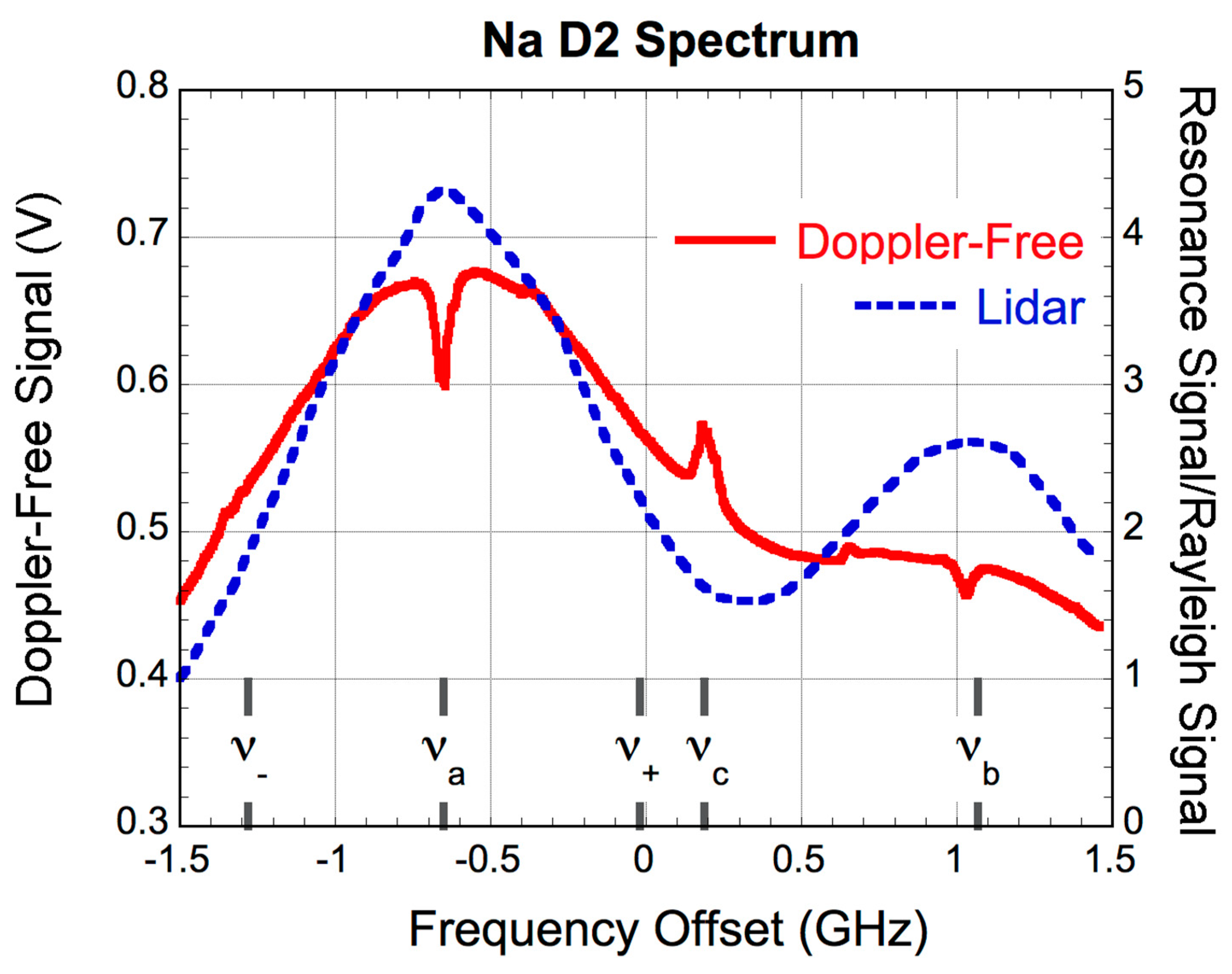
2a peak of the sodium spectrum. The lidar signal from the atmospheric sodium layer clearly follows the amplitude of the laboratory Doppler-free spectrum as the frequency of the CW laser is tuned (
Figure 2). The lidar signal is the ratio of the integrated resonance signal (75–155 km) and the Rayleigh signal (25–35 km). The CW laser is tuned over 3.5 GHz by changing the length of the diode laser cavity piezoelectrically. The PMT signal is used to lock the frequency at the D
2a peak by dithering the frequency of the laser around
± 1.6 MHz every second by applying a small voltage offset (~3 mV) to the CW laser piezo.
The remainder of the cube beam splitter; SHG: second harmonic generator; TDL: tunable diode laser.seed laser beam is sent through the frequency shifter, which can shift the seed laser frequency up by 630 MHz, down by 630 MHz, or leave it unshifted. The two acousto-optic modulator (AOM) crystals are synchronized to shift the SRWTL frequency among the three frequencies every 60 laser pulses. The laser beam out of the frequency shifter has a power of ~200 mW and ~100 mW for the unshifted and shifted frequencies, respectively, due to losses in the AOM crystals. This CW beam from the frequency shifter seeds the PDA. The PDA is pumped by a Nd:YAG laser running at 30 Hz with an average power of 13.5 W. The emitted PDA pulses have a full-width-half-maximum (FWHM) linewidth of 100 MHz. The power output of the PDA is typically 900 mW at the unshifted frequency, and 700 mW at the two shifted frequencies. The PDA is aligned so that the power of the amplified spontaneous emission (ASE) is maintained at a low level of 20–50 mW. The ASE is monitored once every hour during data acquisition by automatically blocking the seed beam into the PDA to measure the lidar profile with the ASE beam. The returned signal from the ASE beam is quite weak due to the lower power and broader (~5 nm) linewidth. The receiver has a 1 nm passband at night and a ~5 pm passband during the day, so it only transmits 20% of the ASE signal at night and 1% of the ASE signal at day. We correct the signal for ASE by subtracting the ASE lidar profile from the seeded lidar profile. This correction is generally small.
The PFRR SRWTL makes simultaneous measurements in two directions. The PDA output beam is expanded to a 20 mm diameter beam and then split into two beams by a 50/50 beam splitter. One beam is pointed in the zenith and the other is pointed 20° off-zenith towards the north by two motor-controlled beam steering mirrors. One telescope is pointed in each of the beam directions to receive the return signal. Initially, the zenith telescope was a 0.61 m Newtonian telescope with a focal length of 1.9 m. The zenith telescope was later upgraded to a 0.91 m reflecting mirror with a focal length of 3.0 m in August 2019. The 20° off-zenith telescope is a 0.91 m reflecting mirror that has the same focal length as the other 0.91 m zenith telescope. The beam steering mirrors align the transmitted beams to the receiver telescopes by maximizing the received signal from the sodium layer. The receiver telescopes are fiber-coupled to an optical chopper that runs at 300 Hz and has a rapid receiver opening time (0.1 ms, ~15 km). The 300 Hz signal is stepped down to 30 Hz to trigger the Nd:YAG laser flashlamps and the Nd:YAG laser Q-switch. The backscattered lidar signal is detected by a PMT that operates in photon counting mode and recorded by a high-speed multi-channel scaler unit. The scaler unit forms the raw lidar signal profile by co-adding the signals from 60 laser pulses. The raw data profiles are then stored on the data acquisition personal computer (PC). The raw lidar signal from each frequency is recorded at a range resolution of 30 m and integrated for 2 s before shifting to the next frequency. A sequence of three frequencies takes about 8 s to acquire and record before the next sequence begins. The ratio technique is then be applied to the recorded lidar signal profiles to retrieve the wind and temperature over the height of the sodium layer [
23,
24]. We use the data analysis program originally developed by Dr. Krueger and Dr. She for the Colorado State University (CSU) and Weber SRWTLs. The analysis of the daytime data takes the ~5 pm wide Faraday Filter spectrum into account [
24,
25].
3. Performance and Efficiency of SRWTL Transmitters
We compare the operating characteristics of the PFRR SRWTL transmitter with seven other previous and currently operating SRWTLs. The previous systems include the original lidar at Colorado State University (CSU) [
9,
26,
27], the lidar at the University of Illinois at Urbana-Champaign (UIUC) (7,8), and the Weber lidar (Weber) [
13,
16,
28]. The original CSU lidar was upgraded from a 20 pps system to a 50 pps system (CSU1 and CSU2, respectively). The current systems are the Utah State University (USU) system, the Andes Lidar Observatory (ALO) system, the University of Science and Technology of China (USTC) system, and the system at PFRR (PFRR). The USU system incorporates the CSU SRWTL (CSU2), which was relocated from CSU to USU in 2010, and was upgraded with a high-power tunable diode laser (DLC TA-SHG Pro, Toptica Photonics AG) as the CW seed laser in 2017 [
29]. The ALO system incorporates the UIUC system, which was relocated to ALO from UIUC in 2009, and was upgraded in 2014 with the same Toptica high-power tunable diode laser as the CW seed laser [
30]. The USTC SRWTL was developed in 2011 and employed a ring dye laser as the CW seed laser [
31]. The UTSC system has recently been upgraded with a Toptica high-power tunable diode laser. The PFRR SRWTL incorporates the Weber sodium lidar, which was relocated to PFRR in 2017, and was upgraded in 2017 with the same Toptica high-power tunable diode laser. We present the characteristics of these seven SRWTLs in
Table 1, where the systems are listed in chronological order of their development.
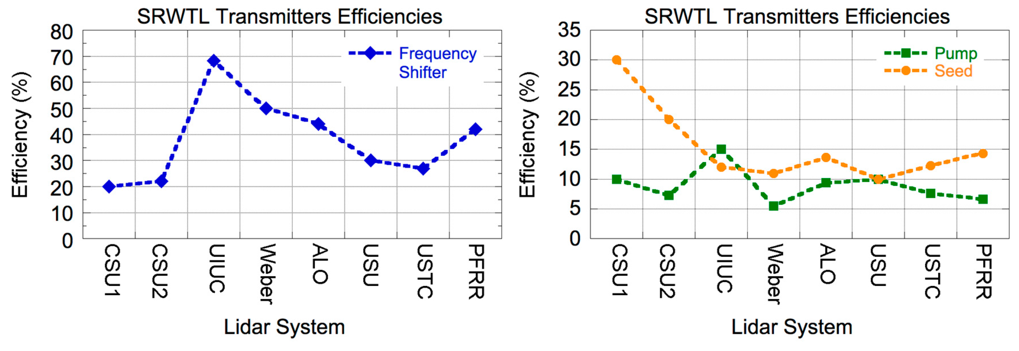
The PFRR SRWTL combines a 500 mW CW seed beam at 589 nm and a pulsed Nd:YAG laser with 450 mJ pulses at 532 nm operating at 30 pps to yield a transmitter with an average output power of 900 mW. The seven other SRWTLS have CW seed beams with powers between 400 and 1000 mW, are pumped by Nd:YAG lasers with pulse energies between 300 mJ and 566 mJ, and have output powers between 600 mW and 1500 mW. We consider the performance of the transmitter in terms of three efficiencies. The first is the efficiency of the frequency shifter and is defined as the ratio of the CW power into the PDA to the power of the CW laser. The second is the PDA pump efficiency and is defined as the ratio of the pump Nd:YAG energy into the PDA and the output pulse energy of the PDA. The third is the PDA seed efficiency and is defined as the ratio of the seed power into the PDA and the output pulse energy of the PDA. For the PFRR system we have a frequency shifting efficiency of 42%, a PDA pump efficiency of 7%, and a PDA seed efficiency of 14%. This compares with values of frequency shifting efficiency of 20–68%, pump efficiency of 5–15%, and seed efficiency of 10–30% for the other seven lidar systems (
Figure 3). The PFRR system has a relatively high frequency shifting efficiency, a typical PDA seed efficiency, and a relatively low PDA pump efficiency. Clearly the area of greatest potential improvement in the PFRR SWRTL transmitter is in the Nd:YAG pumping of the PDA. We are currently investigating the coupling, alignment and optics of the PDA to improve the pump efficiency. We have achieved output power of up to 1.5 W from the PDA, but the ASE was relatively high at ~150 mW, so the challenge is to reduce the ASE while maintaining high seeded laser power.
4. Operational Performance of PFRR SRWTL
We determine the performance of the SRWTL during the Lidar Studies of Coupling in the Arctic Atmosphere and Geospace 1 (LCAGe-1) campaign in the fall of 2018 and LCAGe-3 campaign in the summer of 2019. During LCAGe-1, the PFRR SRWTL obtained both nighttime and daytime measurements of the sodium layer (
Figure 4). We identify two representative signal profiles from the nighttime and daytime measurement to demonstrate the performance of the system on the night of 1–2 October 2018 (day 275 UT). These two profiles are chosen as they had the largest backscattered signal measured in the range of 70 km to 120 km, which we will refer to as the sodium signal hereafter.
We analyze the performance of the system in terms of the uncertainties in the sodium temperature and wind measurements due to the statistics of the photon counting process, which is the dominant source of statistical uncertainty in the lidar signals. The lidar signals are detected by the PMTs, and the statistics of the signal obeys a Poisson distribution where the variance of the signal equals the mean value of the signal [
32]. The temperature and wind are retrieved using the ratio technique. The temperature is derived from the ratio
where
NS(
ν,z) is the total lidar signal at frequency ν and altitude
z,
νa,
ν+, and
ν− are the D2
a, upshifted (
νa + 630 MHz) and downshifted (
νa − 630 MHz) frequencies, respectively,
NB is the background signal, and
zR is the Rayleigh altitude. The corrections for extinction are not included as they cancel out in Equation (1). The wind is derived from the ratio
Given the definition of
and
, we use the propagation of error technique to quantify the uncertainties of
and
as
where
is the lidar signal (total signal minus background) when the laser is tuned to the D
2a line, N
sum is the sum of the upshifted and downshifted signals, and N
diff is the difference in the upshifted and downshifted signals [
24,
33]. To determine these uncertainties, we first integrate the photon counts in both time and altitude (5 min and 1 km) and use this integrated signal as the expected signal. Based on the assumption that the signals obey Poisson distribution, the uncertainty in the signal is then taken as the square root of the expected total signal (i.e.,
). We estimate the background signal by calculating the average lidar signal over the 150–225 km altitude range, where there is no lidar signal from the atmosphere. We then subtract this background from the total signal and obtain the lidar backscatter signal. We calculate the Rayleigh backscatter signal by integrating the backscatter signal profile over the range of 25 km to 35 km. We use this averaged Rayleigh signal to normalize the sodium backscatter signal, and then determine the ratios,
and
. By integrating the Rayleigh signal over a much larger range (10 km) than the sodium signal (1 km), we reduce the relative uncertainty in the Rayleigh signal and thus the uncertainty in the estimate of the temperature and wind ratios are dominated by the uncertainties in the resonance signals. We use Equations (4) and (5) to characterize the uncertainties in these ratios. For the nighttime measurements, the sodium signal is highest at 20:12:27 on 1 October 2018 (05:12:27 on day 275 UT). At the peak of the backscatter signal, 91 km overhead, the sodium number density, temperature, and wind are 4170 cm
−3, 202.4 K, and 0.6 m/s, respectively. The resonance backscatter signal in the zenith beam at the D
2a, upshifted, and downshifted frequencies at the peak of the layer are 1.7 × 10
5, 5.4 × 10
3, and 4.9 × 10
3 counts, respectively. The corresponding Rayleigh backscatter signals are 2.4 × 10
6, 1.7 × 10
6, and 1.7 × 10
6 counts, respectively. The background signals are 44, 40, and 40 counts. The relative uncertainties in
and
are 1% and 20%. The absolute uncertainties in temperature and wind are 1.4 K and 2.2 m/s, respectively. At the peak of the sodium layer 20° to the north, the sodium number density, temperature, and wind are 4045 cm
−3, 201.3 K, and −3.0 m/s, respectively. The resonance backscatter signal in the off-zenith beam at the three frequencies at the peak of the layer are 2.3 × 10
5, 6.8 × 10
3, and 7.5 × 10
3 counts, the Rayleigh backscatter signals are 3.6 × 10
6, 2.6 × 10
6, and 2.7 × 10
6 counts, and the background signals are 25, 25, and 25 counts, respectively. The relative uncertainties in
and
are 1% and 18%. The absolute uncertainties in temperature and wind are 1.1 K and 1.8 m/s, respectively.
For the daytime measurements, the total sodium signal is the highest at 08:21:17 on 2 October 2018 (17:21:17 on day 275 UT). At the peak of the sodium layer, 93 km overhead, the sodium number density is 5460 cm−3. The resonance backscatter signal detected in the zenith beam at the D2a, upshifted, and downshifted frequencies at the peak of the layer are 2.3 × 10³, 5.2 × 10², and 6.6 × 10² counts, respectively. The Rayleigh backscatter signals are 2.4 × 10⁵, 2.2 × 10⁵, and 1.4 × 10⁵ counts, respectively. The background signals are 4.5 × 10³ counts for all three frequencies. The relative uncertainties in and are 9% and 75%. The uncertainties in the temperature and wind are 9.7 K and 6.1 m/s, respectively. In the 20° north beam, at the peak of the sodium layer, 93 km overhead, the sodium number density is 5430 cm−3. The backscatter signal detected at the three frequencies at the peak of the layer are 3.7 × 10³, 6.5 × 10², and 9.9 × 10² counts, the Rayleigh backscatter signals are 4.2 × 10⁵, 3.4 × 10⁵, and 2.3 × 10⁵ counts, and the background signals are 3.9 × 10³ counts for all three frequencies. The relative uncertainties in and and the temperatures and winds are 6% and 28%. The uncertainties in the temperature and wind are 6.7 K and 5.1 m/s, respectively. The increase in the uncertainties in the daytime measurements is due to the decrease in signal due to the insertion loss of the magneto-optic Faraday filter (factor of ~1/7) in the receiver and the increase in the background skylight (factor of ~160).
We compare the nighttime lidar signals from the PFRR SRWTL obtained during the LCAGe-3 with nighttime signals from the USTC SRWTL in 2012 [
31]. We chose the USTC SRWTL for our comparison as it is the most detailed and recent presentation of raw signal profiles for this class of lidars. The USTC SRWTL had the same architecture as the PFRR system. In 2012 the USTC SRWTL incorporated a ring dye laser as the seed laser. The USTC SRWTL lidar has recently been upgraded with a solid-state tunable diode laser. Our comparison is conducted in terms of the resonance signal where we normalize the signals to allow for the transmitter power and receiver aperture. The PFRR lidar has a power of 900 mW, split 50/50 between two beams pointing at the zenith and 20° off-zenith to the north. The upgraded two-direction receiver has one telescope pointing in the zenith and another telescope pointing 20° off-zenith to the north, both with a diameter of 0.91 m. The power aperture product of the lidar in both directions is 0.292 W-m
2. The raw lidar signal measured by the PFRR SRWTL system at 23:44:20 LST on 11 August 2019 (08:44:20, 12 August 2019 UT) represents the lidar signal acquired over 2 s (60 laser pulses) at each frequency at 30 m range resolution (
Figure 5). We retrieved the sodium number density with 1 km zenith and 5 min temporal integration at 08:45 LST as 1780 cm
−3 (zenith) and 1990 cm
−3 (north). The north beam of the USTC lidar has a power of 780 mW, and the receiver telescope has a diameter of 0.76 m, pointing 30° off-zenith to the north [
31]. The power aperture product is 0.354 W-m
2. The east beam of the USTC lidar has a power of 520 mW, and the receiver telescope has a diameter of 0.76 m, pointing 30° off-zenith to the east [
31]. The power aperture product is 0.236 W-m
2. We estimate the raw lidar photon count signal measured by the east and north beams of the USTC SRWTL at 01:30 LST on 23 November 2017 (17:30:13, 22 November 2017 UT) (
Figure 5, [
31]). These profiles represent lidar signal acquired over 40 s (1200 laser pulses) for each frequency at 150 m range resolution. We adopt a representative sodium number density of 3000 cm
−3 measured by the USTC SRWTL two days earlier at 22:15 LST on 20 November 2012 (Figure 8, [
31]).
To compare the PFRR and USTC lidar signals, we compensate the signals for the differences in the pointing angle, the range resolution, the temporal resolution or number of laser pulses, and power-aperture product. The range,
r, and altitude,
z, are related as
where α is the angle off-zenith. The equivalent zenith signal, N
ev, at a given altitude,
z, and resolution, Δ
z, can be determined from the off-zenith signal, N, as follows,
where
r is the range of the measurement and Δ
r is the range resolution of the measurement. We first calculate the lidar signals normalized by the number of laser pulses at the peak of the sodium layer (N
S) (
Table 2). At PFRR the sodium layer peak is detected at 89 km in both beams while at USTC the peak is detected at 92 km in the east beam and 88 km in the north beam. We convert these to equivalent signals at 90 km (N
Sev) for 1000 laser pulses. We normalize these signals by the power-aperture product and obtained a quality factor, Q
s, and then normalize Q
s by the sodium number density to obtain the quality factor Q
ρ independent of the sodium concentration. We use both Q
s and Q
ρ to compare the efficiency of the two lidar systems.
Examining the relative efficiencies (Qs and Qρ) of the PFRR SRWTL, we see that the north receiver is 40–50% as efficient as the zenith receiver. When we compare the PFRR and USTC systems, the values of Qs indicate that the PFRR zenith receiver is 88–97% as efficient as the USTC system and the north receiver is 43–47% as efficient as the USTC system. The values of Qρ indicate that the PFRR zenith receiver is 143–165% as efficient as the USTC system and the north receiver is 61–70% as efficient as the USTC system. The USTC sodium concentration was measured two days earlier than the photon count profiles, and we picked the maximum number density (3000 cm−3) from that night to calculate Qρ. Thus, the Qρ we presented for the USTC system is a conservative value. Based on these analyses, we find that the zenith receiver of the PFRR lidar is operating with a slightly lower efficiency than the USTC system. This lower efficiency may be attributed to differences in the age of the detectors where the PFRR system has older PMTs than the USTC system. The lower efficiency of the PFRR north receiver relative to the zenith receiver may be attributed to misalignment of the coupling fiber in the north receiver that requires further optimization.


