Article

Teleconnection of Regional Drought to ENSO, PDO, and AMO: Southern Florida and the Everglades

1
Department of Earth and Environment, Florida International University, Miami, FL 33199, USA
2
Water and Environment Consulting LLC, 6153 Terra Rosa Circle, Boynton Beach, FL 33472, USA
*
Author to whom correspondence should be addressed.
Atmosphere 2019, 10(6), 295; https://doi.org/10.3390/atmos10060295
Submission received: 6 May 2019 / Revised: 18 May 2019 / Accepted: 25 May 2019 / Published: 30 May 2019

Abstract

:
Drought variability is associated with global oceanic and atmospheric teleconnections driven by, among others, the Pacific Decadal Oscillation (PDO), the Atlantic Multidecadal Oscillation (AMO), and El Niño–Southern Oscillation (ENSO). Climate teleconnections with a region’s rainfall, with drought and flooding implications, should be part of short- and long-term water management planning and operations. In this study, the link between drought and climatic drivers was assessed by using historical data from 110 years of regional rainfall in southern Florida and the Everglades. The objective was to evaluate historical drought and its link with global oceanic and atmospheric teleconnections. The Standardized Precipitation Index (SPI) assesses regional historical drought in 3-, 6-, 12-, 24-, 36-, 48-, and 60-month periods. Each of the SPIs was used to analyze the association of different magnitudes of drought with ENSO, AMO, and PDO. Historical drought evaluated in different time windows indicated that there is a wet and dry cycle in the regional hydrology, where the area is currently in the wet phase of the fluctuation since 1995 with some drought years in between. Regional historical rainfall anomaly and drought index relationships with each driver and combination of drivers were statistically evaluated. The impact of ENSO fluctuation is limited to short-period rainfall variability, whereas long-period influence is from AMO and PDO.

1. Introduction

Ocean–atmosphere interactions are known for regulating global energy flow that influences rainfall amounts and distribution on a regional scale [1,2,3]. The link between these drivers, rainfall pattern, and general hydroclimate variability has been a focus of several studies on a regional scale [2,4,5,6,7,8,9,10]. For example, the magnitude, spatial, and temporal distribution of rainfall in the United States are a function of different modes of ocean–atmosphere interaction processes, as well as other global and regional conditions. In Southeast Florida, the Pacific Decadal Oscillation (PDO), the Atlantic Multidecadal Oscillation (AMO), and El Niño–Southern Oscillation (ENSO) influence rainfall variation [1,2,11,12]. A detailed study based on 11 stations in Florida, including Southeast Florida, showed AMO–ENSO coupled influence on rainfall and concluded that AMO (cool) and ENSO (El Niño) created wetter conditions than AMO (warm) and El Niño combination [13]. In a study of precipitation and climate teleconnections in the Greater Everglades and South Florida, it was reported that the dry season is correlated to ENSO and that AMO influences wet season rainfall [14]. A study using historical water clarity and climate teleconnections in Lake Annie in Central Florida reported that water clarity was higher during the AMO cold phase and lower during the AMO warm phase with a decrease and an increase in rainfall, respectively [15].
Although these ocean–atmosphere interaction modes are regional processes with a broad global influence, the net effect of these processes on rainfall distribution varies by region. Therefore, for a regional water resource management system, understanding the link between the individual and combined effects of the drivers at the regional scale is essential. The Everglades wetland system, a unique and complex ecohydrology, has been facing stress from water quality degradation and change in magnitude and distribution of supply. As a result, a state and federally supported ecological restoration program was initiated in the early 1990s [16]. In southern Florida, the water supply of the Everglades wetland system and the highly populated Miami-Dade County (Figure 1), is subject to hydroclimate variations.
South Florida is home to more than 6 million people and to the Everglades ecosystem. The Everglades is a unique freshwater marsh that has ecological and water supply importance covering over 5500 km2 in its current reduced state. The urban water source is the Biscayne Aquifer, a shallow unconfined freshwater aquifer system. The Biscayne Aquifer covers southeastern Florida including parts of Palm Beach, Broward, Miami-Dade, and Monroe counties. Groundwater recharge to the aquifer is from rainfall and runoff, canal recharge, and from the Everglades wetland. Due to increased pumping pressure and increasing water demand, the recurrence of droughts is frequently compromising the sustainability of the aquifer. This has increased the dependence of the aquifer on recharge from the Everglades and from upstream canals. Groundwater head decline due to pumping pressure and declining rainfall conditions is threatening the health of the aquifer, as well as the Everglades ecosystem from increased salinity.
Rainfall is a significant source of freshwater input into the region’s freshwater balance. Precipitation is driven by local and regional hydroclimate factors [12]. In addition to regional ocean–atmosphere interaction, the region’s geographic location in juxtaposition to the Atlantic ocean (Figure 1) and the presence of the Everglades wetland hydrologic system have significant influence over the local rainfall distribution in the area [17]. As a result, the area receives rainfall driven from local and regional climate circulation factors, convective rain, tropical depressions and storms, and frontal rainfall systems [18].
Extreme hydrologic events, such as droughts to high-intensity rainfall, are frequently observed in the region. Particularly, droughts along with other water demands pose a challenge to the continuous supply of freshwater to the Everglades. Apart from intense competition for the use of the fully allocated water resource system, drought has presented a threat to sustained freshwater availability in the Everglades. In South Florida, drought has been recorded in the years 1932, 1955–1957, 1961–1963, 1971–1972, 1973–1974, 1980–1982, 1985, 1988–1989, 1990, 2000–2001, 2006–2007, and 2011–2012 [19,20,21]. These drought events have caused a remarkable decline in surface and groundwater head, and a significant disturbance to the Everglades ecosystem [22,23,24,25,26]. In general, short- and long-term drought has been observed in different periods whose effect varies with duration and magnitude of the rainfall deficit [12,24,27].
The teleconnections between ENSO and rainfall in South Florida is well known and accepted. Short-term drought events have a strong association with La Niña [1,25]. El Niño results in an increase in dry season rainfall. However, small-scale and persistent rainfall deficit is a function of low-frequency ocean–atmosphere interaction modes, namely, PDO, AMO and others. Regional rainfall variability is a function of the interaction between low-frequency and high-frequency ocean–atmosphere interaction modes. Therefore, evaluating rainfall deficit in different time windows and the association between rainfall deficit and individual and combined effects of the ocean–atmosphere interaction modes is necessary to manage regional water sustainably in South Florida [28]. With respect to the degree of rainfall association with the different ocean–atmosphere interaction modes, the current state of the fluctuation in the region is well evaluated; however, the possible implications for long-term freshwater availability at the regional scale have not been evaluated sufficiently. Therefore, the objectives of this study were the following: (1) assess historical droughts in the region, (2) evaluate the link between each of the regional hydroclimate drivers (ENSO, AMO, and PDO) and rainfall variability in the region, and (3) define the combined effects of the ocean–-atmosphere interaction modes on regional drought. An understanding of the relationship between regional droughts with regional ocean–atmosphere interaction modes aids short- and long-term water resource management planning and decision-making. Furthermore, such knowledge can be applied to promote long-term drought preparedness and response. Accordingly, in this study, the correspondence between regional rainfall anomaly and each of the drivers’ indices is presented as a pairwise correspondence analysis. Then, historic droughts in the region for different time scales are shown. Finally, the combined effect of the drivers on drought in the region is presented. Implications for the current and future water resource availability, water resource management alternatives, and management priorities under drought conditions are discussed.

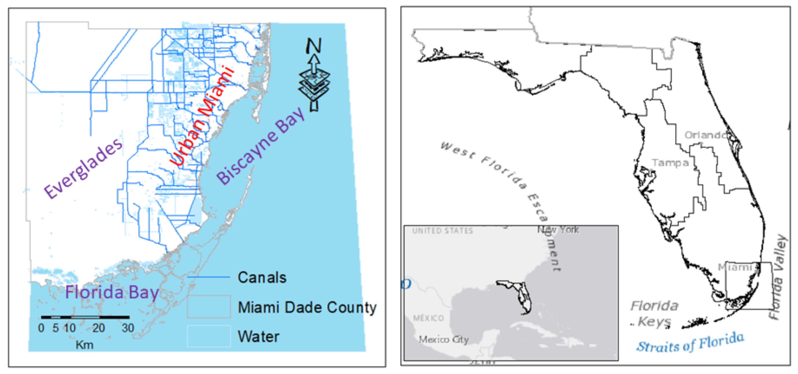
2. Dataset and Study Area
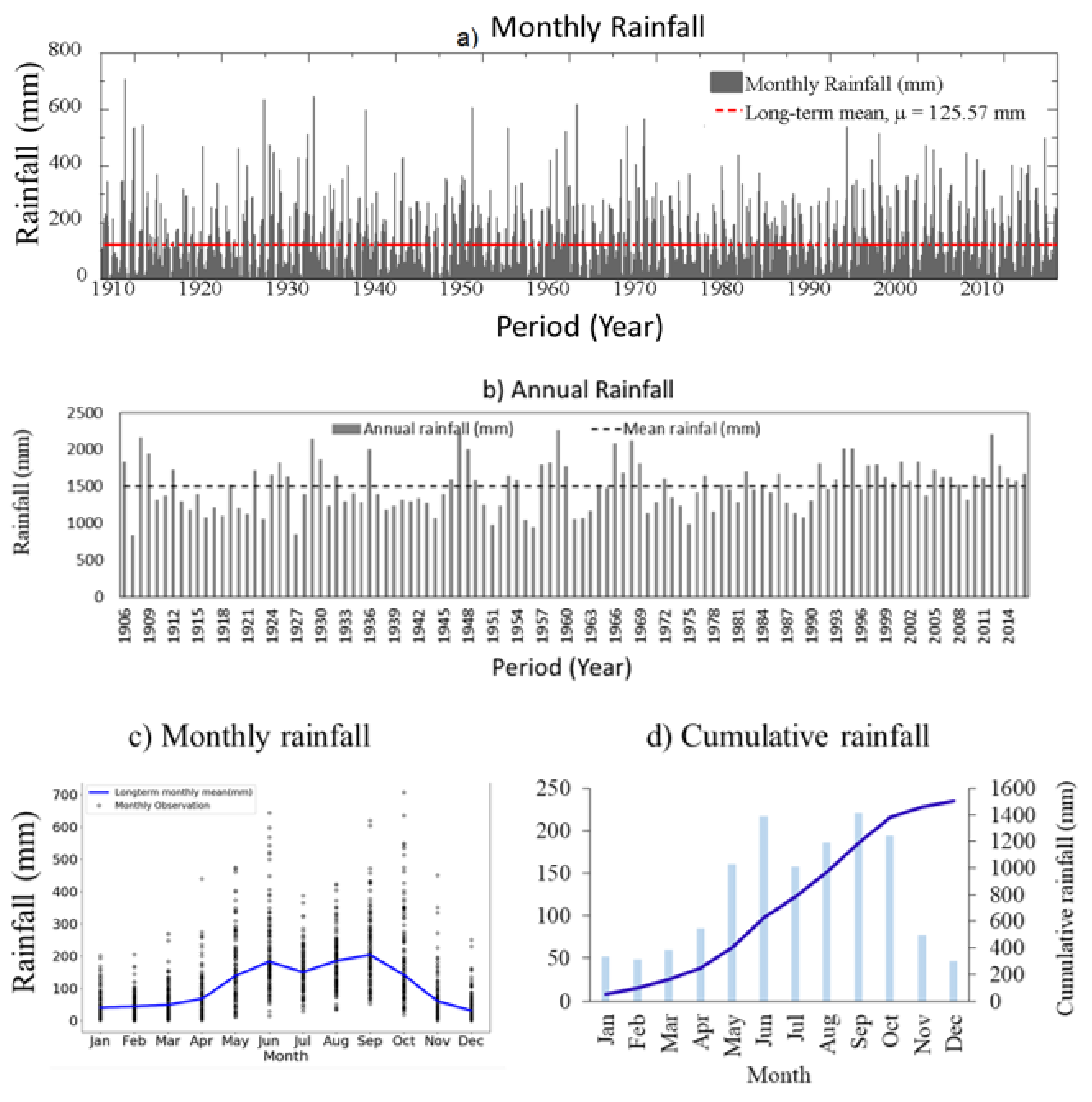
2.1. Rainfall

Long-term monthly regional rainfall data, from 1906 to 2016 (Figure 2a), were accessed from the Florida climate center [29]. This regionalized monthly rainfall data were derived from a number of ground-based rainfall measurement stations. The regionalization has combined historical records from the National Weather Service’s Cooperative Observation (COOP) network and the Automated Surface Observing System (ASOS). In South Florida, monthly rainfall measurement can be represented by a station for an area having approximately an 80 km radius [18,30]. Monthly rainfall variation has a wide range, that is, a 10–100 km spatial scale [14]. Therefore, these data are considered as a representative monthly rainfall for the Southeast Florida regional scale. The mean annual rainfall in the study area is 1507 mm (Figure 2b) compared to the mean rainfall for the Everglades National Park of 1386 mm (1941–2016) [21].
The long-term mean monthly rainfall of 125.57 mm (Figure 2a) defines Southeast Florida as one of highest rainfall-receiving regions. Seventy-five percent of the annual rain in the region occurs in the wet season [27]. The mean monthly long-term rainfall is characterized by a bimodal rainfall distribution (Figure 2c,d), where June and September are peak rainfall months and the cumulative mean monthly rain indicates that November–April is the dry season while May–October is the wet season (Figure 2c). A thorough statistical evaluation of the same dataset has indicated a decreasing trend of the wet season duration leading to the emergence of a unimodal rainfall regime [27].

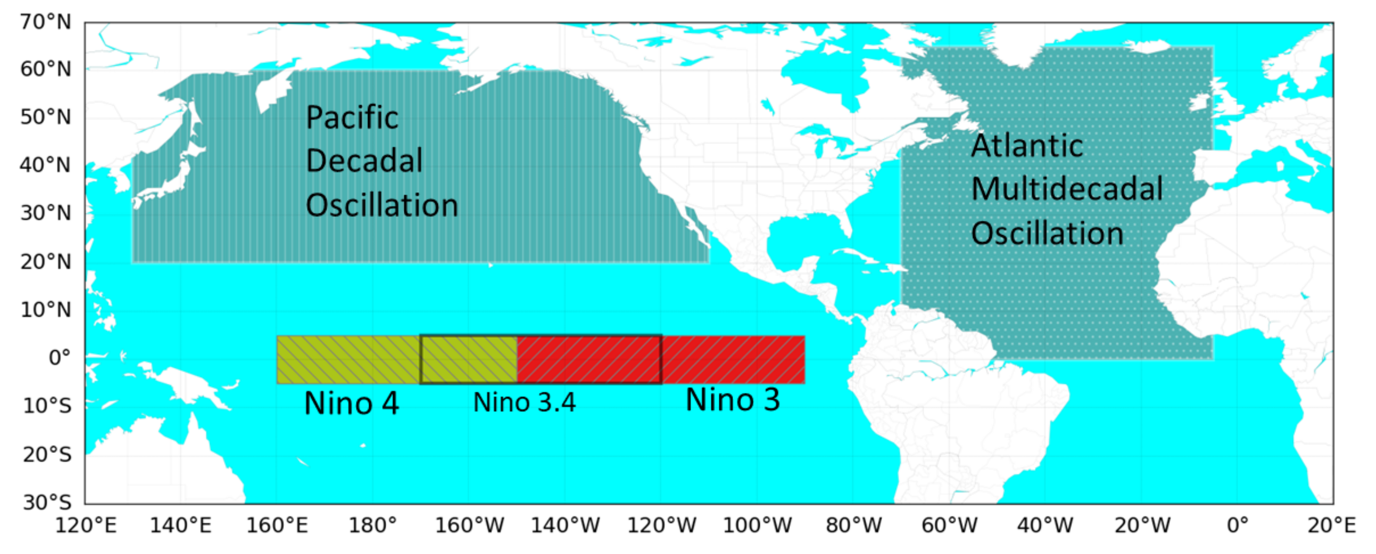
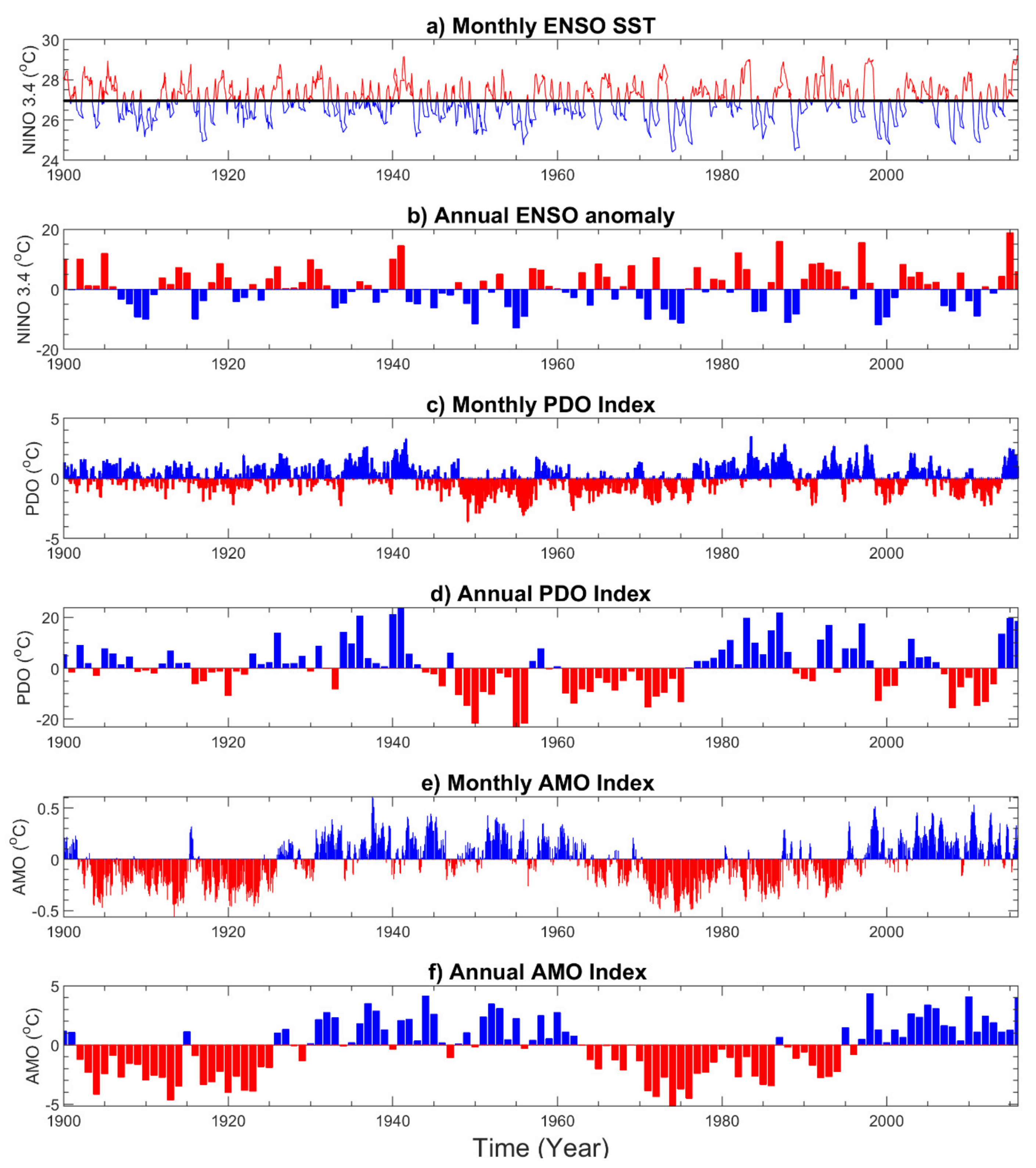
2.2. ENSO, PDO, and AMO Dataset

ENSO is a natural ocean–atmosphere interaction process defined by sea surface temperature (SST) variations measured in the eastern and central equatorial Pacific. The SST anomaly in the tropical Pacific region (5° N to 5° S, 170° W to 120° W) refers to NINO 3.4 (Figure 3), which corresponds to hydrological variation in the USA [31,32,33].
Based on the equatorial Pacific SST anomaly, ENSO has three phases. El Niño is the result of the weakening of the easterly trade winds. This weakening allows the development of a positive SST anomaly in the eastern equatorial Pacific Ocean. On the other hand, the persistence of easterly trade winds pushes the warm pool to the west, causing an upwelling of cooler water in the eastern equatorial Pacific Ocean. The upwelling results in cooler than average SST in the eastern and central equatorial Pacific (negative SST anomaly), resulting in a La Niña condition. The presence of equatorial SST close to normal, within ±0.5 °C, is a neutral phase of ENSO. In Southeast Florida, the positive SST anomaly, El Niño (SST > 0.5 °C), is associated with an increase in dry season precipitation, whereas La Niña (SST < −0.5 °C) is associated with drought in the dry season [1]. ENSO has a 3- to 7-year cycle, whereas the effect of El Niño or La Niña can persist for 6 to 18 months [27].
The standard format monthly Nino 3.4 data was accessed from the National Oceanic and Atmospheric Administration’s Climate Prediction Center [34] (Figure 4a). In this study, the monthly and total annual ENSO anomalies (Figure 4b) are calculated as residual from the long-term normal.
PDO is an index of the SST change in the Pacific Ocean poleward of 20° North. Similar to ENSO, the changes in SST, sea level pressure, and wind pattern in the northern Pacific Ocean influence a greater area in continental North America and the rest of the world. PDO with a 5- to 30-year cycle has an effect similar to ENSO on the rainfall distribution in the continental U.S. [7,35]. However, unlike ENSO, it has a low frequency and hence the net effect of PDO over an area for a given time is a function of the nature of the superposition between ENSO and PDO. For example, studies indicate that when PDO and ENSO are in phase, PDO can be constructive to the effects of ENSO [31,36].
For this study, the PDO index data from 1906 to 2016 (Figure 4c,d) were accessed from the Joint Institute for the Study of the Atmosphere and Ocean (JISAO) at the University of Washington [37]. This database exhibits the standardized PDO index derived from monthly SST anomalies.
Representing the mean SST changes in the North Atlantic Ocean from 0° to 60° N, AMO is characterized by multidecadal variability with 40-year cycles with a maximum full duration of up to 70 years [7,10,11,38]. Therefore, an important hydroclimate variable controls the long-term precipitation pattern. The AMO anomaly has an inverse relation with precipitation amount in some regions of the U.S., where the warm (cold) phase of AMO is associated with dryness (wetness) [7]. The AMO index is a measure of the 10-year running average of SST anomalies in the North Atlantic Ocean. The AMO index (Figure 4e,f) used in this study was accessed from the Kaplan SST dataset available online (https://www.esrl.noaa.gov/psd/data/timeseries/AMO/) [7]).

3. Methodology

3.1. Correspondence of Regional Rainfall Anomaly to ENSO, AMO, and PDO

The monthly rainfall anomaly is the deviation from the long-term normal of each corresponding month. The monthly rainfall residual was used to develop a year–month matrix that was plotted using empirical Bayesian kriging (EBK) as indicated in previous studies [27]. The pattern of the rainfall residual chart was compared to ENSO, PDO, and AMO charts developed by the same approach.
The quadrant-based paired point-count approach was used to evaluate the degree of correspondence or synchronicity between the total annual and dry season rainfall anomaly and ENSO, PDO, and AMO. The method was used to statistically evaluate the significance of the correspondence portrayed in the monthly rainfall anomaly analysis chart. The yearly and dry season rainfall anomalies were plotted against ENSO, PDO, and AMO. The diagram obtained indicates the location of each contemporaneous pair in one of the four quadrants (QI to QIV). The correspondence is the count of positive–positive (QI-true positive) and negative–negative (QIV-true negative) pairs. The true positive counts indicate the increase in rainfall with the positive anomaly of each of the drivers, and the true negative counts indicate the decrease in rainfall with the negative anomaly. The pairs at quadrant II (QII, false negative) and quadrant III (QIII, false positive) indicate that the change in the drivers does not represent the rainfall anomaly.
The strength of association between rainfall anomalies with each of the drivers was computed and compared using chi-squared test statistics [1,28]. Using this approach, one can assess the degree of correspondence between the cumulative annual anomalies (sum of the monthly anomaly) of ENSO with the total dry season (November to May) rainfall anomaly. It is presented as a test of significance of binomial proportions, chi-squared test (Equation (1)). This analysis (Equation (1)) is based on the hypothesis that there is a correspondence between the cumulative dry month’s rainfall and each of the drivers [1]:
χ 2 = i = 1 2 ( f i F ) 2 F ,
where χ2 is the chi-square of the binomial proportions; f1 + f2 is the number of years of the analysis; f1 is the number of years where the rainfall anomaly corresponds to each of the drivers (total counts in QI and QIII); f2 is the number of years where the rainfall anomaly does not correspond to each of the drivers (total counts in QII and QIV); and F is the expected frequency of random correspondence assuming a probability (p) of 0.5, (F = (f1 + f2) P). F is also the expected number of years where the rainfall anomaly does not correspond with any events as p is 0.5.

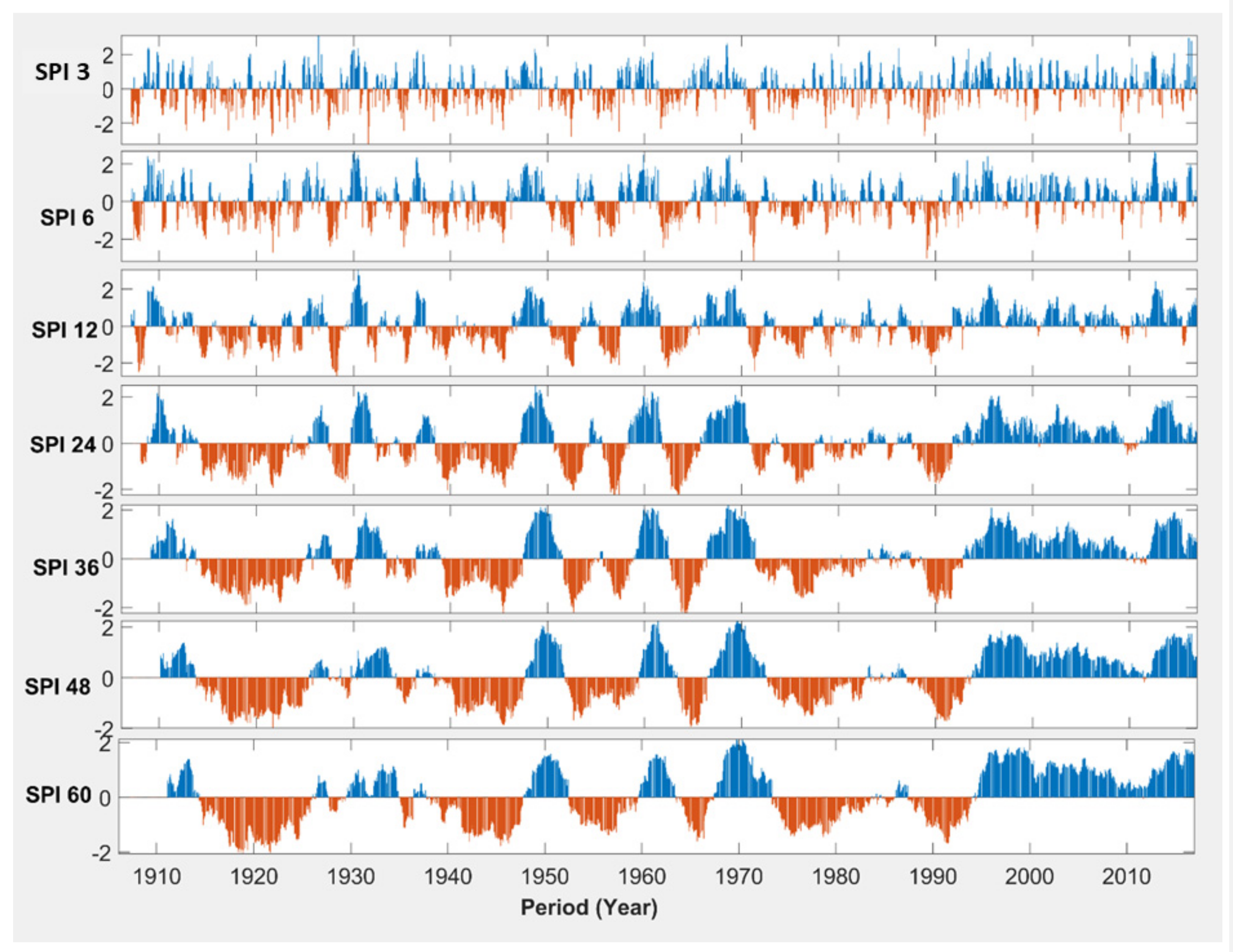
3.2. Drought Evaluation with the Standardized Precipitation Index (SPI)

The regionalized monthly rainfall record from 1906 to 2016 was used to evaluate the drought variability using the SPI in 3-month to 60-month time windows. Monthly regional rainfall data in the region have a gamma probability [27]. Rainfall with a gamma probability distribution can be effectively used to calculate the SPI as given by [39,40,41,42]:
S P I = t c 0 + c 1 + c 2 t 2 1 + d 1 t + d 2 t 2 + d 3 t 3 , t = ln 1 H ( x ) 2 , 0 < H ( x ) 0.5 t c 0 + c 1 + c 2 t 2 1 + d 1 t + d 2 t 2 + d 3 t 3 , t = ln 1 1 H ( x ) 2 , 0.5 < H ( x ) < 1 ,
where c0 = 2.515517, c1 = 0.802853, c2 = 0.010328, d1 = 1.432788, d2 = 0.189269, and d3 = 0.001308.
The SPI (Equation (2)) calculates the incidence of drought over different time windows using the running total rainfall of the respective time windows. For such long-term studies, drought evaluation with the SPI is feasible as it uses rainfall data only [42]. The SPIs (Equation (2)) in different time windows were calculated in the MATLAB (R2018b, MathWorks Inc, Natick, MA, USA) interface. The evaluation of the drought index for an extended period (such as 48 and 60 months) is credible only if the study applies long-period monthly rainfall data [42]. In this study, 110 years of monthly rainfall data were used.
The SPI calculated at 3-, 6-, 12-, 24-, 36-, 48-, and 60-month time windows was used to evaluate the combined effects of ENSO, AMO, and PDO on drought. The SPI analysis result was normally distributed; therefore, the regression analysis could be effectively applied. Each of the sequential time series drought indices calculated by the SPI was used as dependent variables, whereas ENSO, AMO, and PDO all together were used as independent variables. The significance of the strength of each of the independent variables as a driver for regional drought was assessed by t-test statistics evaluated at 95% confidence interval.

4. Results and Discussion

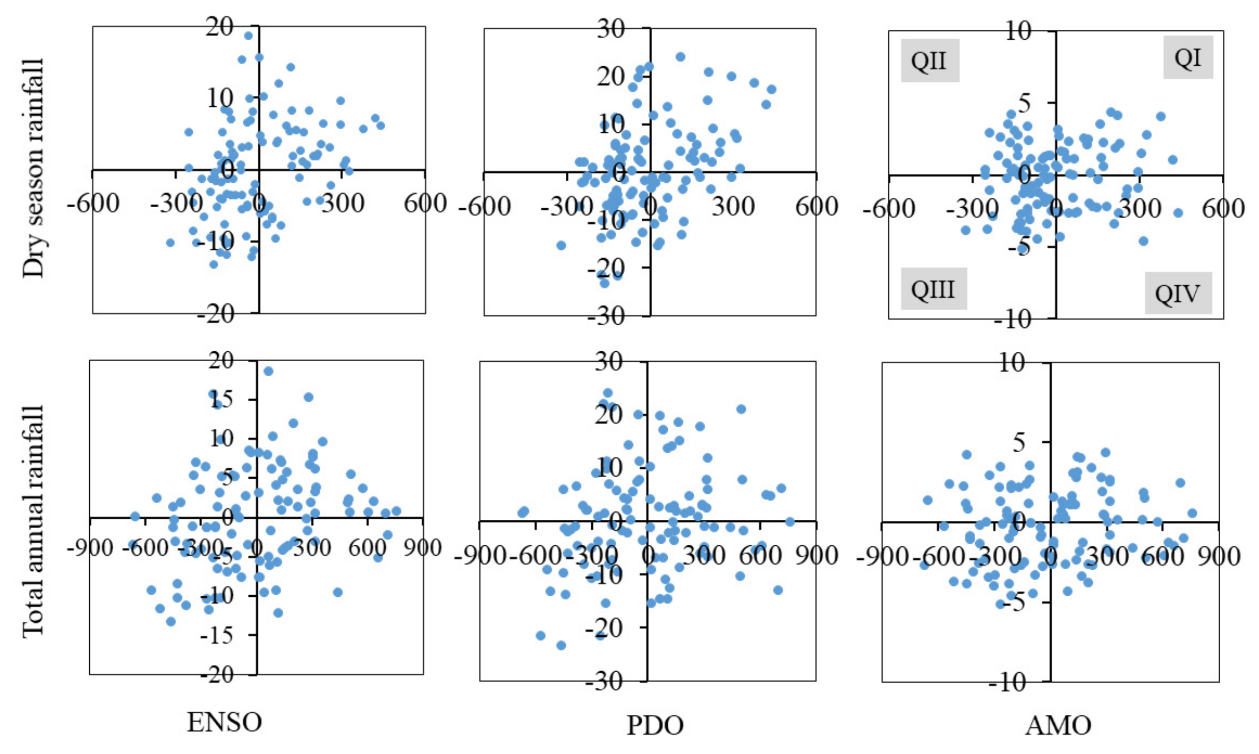
4.1. Pairwise Correspondence Test

Rainfall deviation from the long-term normal is a preliminary indicator of rainfall variability in the area (Figure 5). The residual map represents the difference between the recorded total monthly rainfall and the respective long-term mean monthly value. The residual embodies the overall wetness or dryness of each month as compared to the long-term mean of the respective individual month. Likewise, the plots of ENSO, AMO, and PDO show the coincidence of residual rainfall pattern with the ocean–atmosphere interaction modes.
The residual rainfall chart presents three patterns of the rainfall deviation from the normal. The first pattern is when all months in a year and successive years are wetter than normal. The second pattern is when the dry season becomes wet and the wet season wetter, and the third pattern is when all months are dry. Dryness over a range of years from 1911 to 1923, 1937 to 1945, 1950 to 1958, 1961 to 1963, and 1970 to 1990 are indicated (Figure 5a). On the other hand, the periods from 1908 to 1910, 1928 to 1931, 1945 to 1949, and 1964 to 1969 were wet years, and the contemporary rainfall pattern since the early 1990s indicates sustained wetness except for the incidence of shorter droughts.
The regional rainfall residual chart lacks an authentic similarity with the ENSO variability. The lack of one-to-one correspondence between rainfall deviation and ENSO variability signifies that the rainfall pattern in the area is the cumulative effect of other drivers and external factors. Unlike the ENSO, there is relatively less correspondence of the regional monthly rainfall deviation in the region with the PDO index as the frequency is lower (Figure 5a,c,d).
On a longer timescale, the rainfall residual has high similarity to AMO (Figure 5c). For example, the dryness in early 1911 to 1923 and 1970 to 1990 corresponds to the negative phase of AMO. The long-held wetness from 1990 onward corresponds to the positive phase of AMO. However, the high-frequency rainfall variability between 1925 and 1970 does not show similarity with the long-held positive phase of AMO.
Plotting the rainfall anomalies against the cumulative SST anomalies of each of the indices defines the level of correspondence between rainfall and the drivers (Figure 6). It is evident that South Florida is highly affected by tropical storms causing rainfall outliers. Therefore, it is advised to use dry season rainfall anomalies. Nevertheless, an additional analysis for total annual rainfall deviations evaluates how much of the variation can be attributed to the climate indices.
Dry season anomaly correspondence with ENSO is 73 events out of 110 (QI + QIII) and annual anomaly has a correspondence of 70 events out of 111 (QI + QIII) (Table 1 and Table 2). Accordingly, this correspondence between the rainfall anomaly and ENSO index signifies that ENSO is 63.4% and 63.1% for dry season and annual rainfall variation, respectively. AMO is the second major driver for the rainfall variability in the region. The dry season and annual rainfall anomaly correspondences with the AMO index are 54 out of 110 events and 56 out of 111 events, 49% and 50.1%, respectively. The rainfall anomaly correspondence with the PDO index shows a correspondence of only 52 out of 110 events (43.3%) for dry season rainfall and 55 out of 111 events for annual rainfall (50%). The total annual and dry season rainfall is weakly associated with PDO.
The binomial proportions statistics test assesses the possibility that the paired events are random or have a cause-and-effect relation showing that the chi-square measures the significance of the binomial proportion (correspondence) [1,28]. This analysis shows that ENSO has statistically significant correspondence to both the total annual and the dry season rainfall anomalies (Table 2). Furthermore, ENSO fluctuations have the highest chi-square value for the dry season rainfall (with 95% confidence interval). The dry season negative rainfall anomaly has the most frequent overlap with ENSO on the true negative quadrant of the paired plot. Likewise, the annual rainfall variability is significantly associated with ENSO variability. Accordingly, the most significant driver for the regional rainfall variability is the ENSO fluctuation.
In Table 2, the expected random correspondence of dry season or annual rainfall has a probability of greater than 50% with a chi-square significance value of 5% at one degree of freedom. The AMO index shows a higher degree of correspondence to the total annual rainfall (with 80% confidence interval and tabular chi-square of 1.64) than the dry season rainfall in the region. The chi-square value for the correspondence between PDO and rainfall anomalies in the region indicates a general weaker relationship.
Overall, the rainfall deviation indicates high- and low-frequency signals. ENSO fluctuation influences the short-term variability, whereas the long-held low-frequency signal has high similarity to AMO. An insignificant correspondence between PDO and rainfall anomaly suggests that there is a minimal PDO effect on short-term rainfall variability in the region. This analysis appeals to the need for evaluating the degree of correspondence between the rainfall deviation and each of the drivers. Knowledge of the level of correspondence between each of the drivers is necessary for short-term water management decision-making. However, for sustained long-term water management planning, it is valuable to understand the combined effect of the drivers on regional drought.

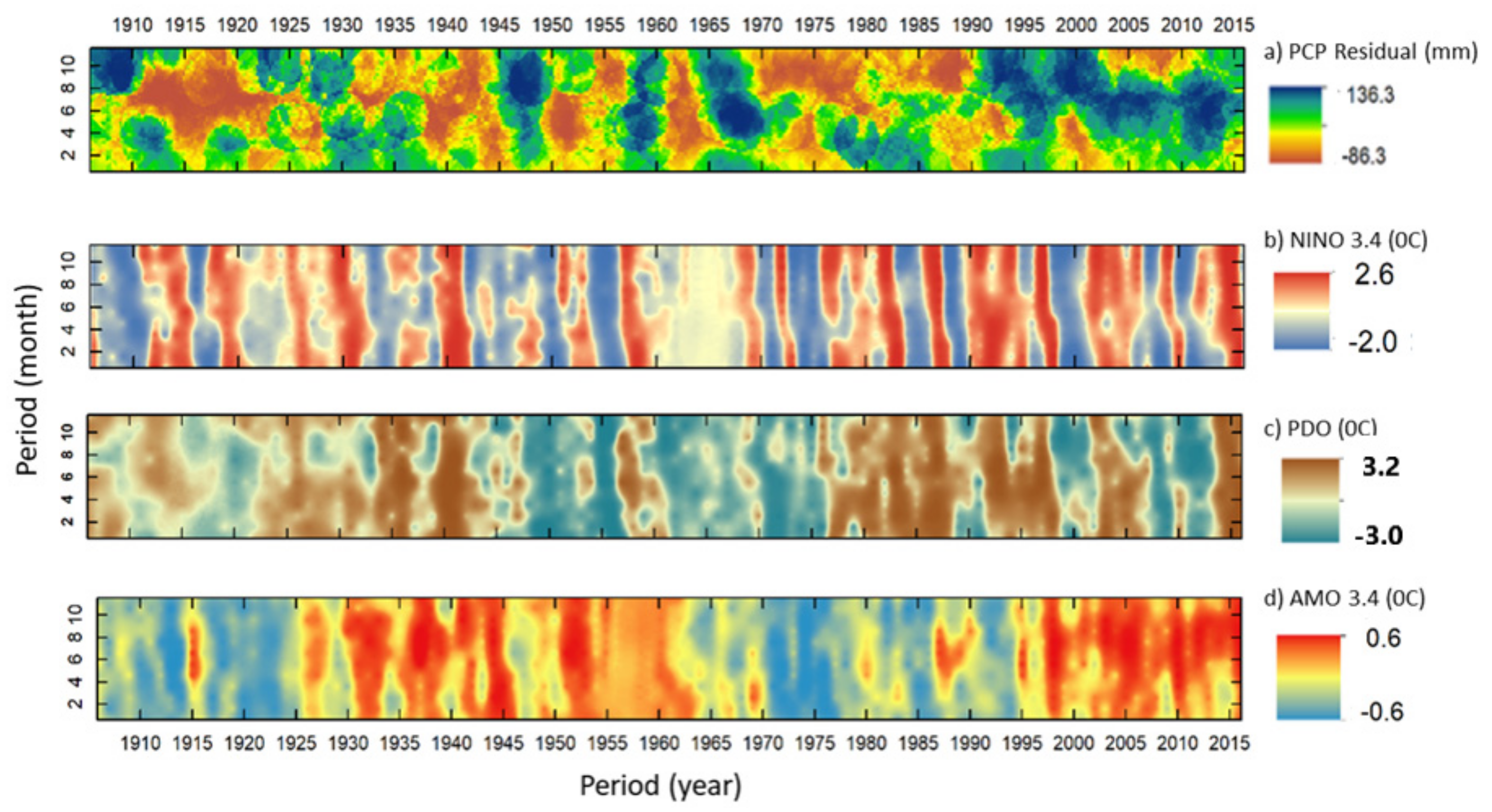
4.2. Combined Effects of Drivers on Regional Rainfall Variability

The results of the SPI indices in 3-, 6-, 12-, 24-, 36-, 48-, and 60-month windows were used for multiple regression analysis of each of the indices against the drivers all together.
The SPI-3, SPI-6, and SPI-12 represent the link between rainfall variability and the drivers, whereas SPI-24, SPI-36, SPI-48, and SPI-60 represent the link between long-term drought and the combined effect of the drivers.
The SPI analysis (Figure 7) agrees with the recorded droughts in the region. Prolonged droughts were observed in 1932, 1955–1957, 1961–1963, 1971–1972, 1973–1974, 1980–1982, 1985, 1988–1989, 1990, and 2000–2001 [24]. Despite the incidence of droughts, such as in 2010–2012, 2014, and 2015, the current hydrology in the area is at the wet phase of the long-term natural dry and wet cycle. An analysis of the drought cycle using fast Fourier transform and input data of the monthly SPI indices indicated that the regional drought has cycles of 2 to 3, 5 to 6, 9 to 10, and 10 to 20 years [27]. Such cycles coincide with the known cycles of ENSO, AMO, and PDO.
In Figure 7, from a bi-annual to a five-year basis, major extended drought is observed from 1914 to 1927 and from the early 1970s to 1995/1996. Between 1940 and the early 1970s, the SPI indicates a clear cyclic pattern of the wet/dry fluctuations in the area. The multiple regression analysis used to evaluate the combined effect of the drivers on different intensities of drought indicates that the ENSO fluctuation has a strong association with SPI-3, SPI-6, and SPI-12 (Table 3). Rainfall variability evaluated by SPI-3 and SPI-6 are the reflections of seasonal fluctuation, whereas negative (positive) values of the SPI-12 refer to the presence of yearly sustained dryness (wetness). Hence, the signature of ENSO fluctuation in the regional hydrological variability is significant as compared to all the drivers. This line of analysis corroborates with the pairwise correspondence test that the dry season rainfall has the highest degree of correspondence to ENSO variability. Hence, the overall yearly rainfall gain or loss attributed to ENSO fluctuation is a function of the impact on the dry season rainfall. If the dry season has more rainfall (ENSO positive), the overall annual rainfall is at or above average.
AMO fluctuation has shown a statistically significant correlation with SPI-6 to SPI-60. Only AMO has shown a statistically significant relationship with the regional rainfall variabilities for over 3 to 5 years, namely, SPI-36, SPI-48, and SPI-60. As indicated in the pairwise association test, unlike ENSO, AMO has shown the strongest association with the total annual rainfall variability than with the dry season rainfall variability. The region receives more than 70% of the total annual rainfall in the wet season. Therefore, that fact that AMO has a statistically significant correlation with the long-term total annual rainfall in the area indicates that AMO variability is an important driver of the long-term (low-frequency but sustained) rainfall variability in the region.
The overall drought analysis using SPI-12 and higher time windows indicates that the region is in an extended wet phase of the rainfall variabilities. Furthermore, the multiple regression indicates that the long-term rainfall variabilities are related to AMO fluctuations, where the positive AMO is in favor of wetness in the region. However, studies indicate the emergence of negative AMO [43].

4.3. Implications for Long-Term Freshwater Management

For a sustainable freshwater management system in the area, it is essential to know the combined effects of AMO and ENSO interactions on hydrometeorology of the region. Four combinations of AMO and ENSO anomalies can control the rainfall and freshwater input to the regional system. The first is the combination of a positive AMO and positive ENSO (El Niño) conditions. The interaction of the positive–positive index is a wet hydrologic regime in the region. This first scenario can be associated with flooding and high-intensity rainfall. The second scenario is a combination of a negative ENSO given positive AMO. A negative ENSO given positive AMO can be a drought on a short time scale. In general, the second scenario can be defined by the recurrence of droughts in the area. The first two scenarios represent the contemporary hydrologic regime in the region, particularly since the early 1990s. Within these two scenarios, the region receives rainfall much more than average. However, negative ENSO corresponds to observed droughts.
Major extended drought episodes in the area coincide with the cold phase of AMO; likewise, the extended wetness since 1994–1995 overlaps with the warm phase of AMO. The third and fourth scenarios are associated with the potential emergence of a negative AMO [31]. The highly likely scenario of the future hydroclimate regime in the region is the balance between long-term droughts induced by negative AMO that is moderated by the frequent recurrence of positive ENSO. Negative AMO has an effect on declining regional rainfall regime. The positive ENSO during negative AMO might help to minimize the adverse effects of rainfall deficit. The occurrence of negative ENSO and negative AMO is the worst-case scenario where drought can be persistent.
Given the possibility of AMO shifting to a negative phase [43,44], the rainfall regime in the region can shift to moderate to severe drought for an extended period. There is a high potential for the emergence of long periods of small-scale droughts. Prolonged small-scale drought effect increases gradually and eventually influences sustainability of the water resource system. This can affect freshwater availability in the Everglades, disrupting the regional ecosystem and ecosystem services. Furthermore, long-term drought can reduce the groundwater head in the Biscay Aquifer, compromise the sustainable yield of the aquifer, and promote saltwater intrusion. Therefore, considering climate teleconnection in regional water management planning and decision-making is a necessity. The South Florida Water Management District has been incorporating climate prediction into its weekly water management decision process using weekly reported climate teleconnection indices [27,42].

5. Conclusions and Recommendations

The evaluation of the correspondence between dry season and annual rainfall with ENSO, AMO, and PDO indicated that ENSO fluctuations have a direct relation to short-term rainfall variability in southern Florida. The multiple regression tests further explained the fact that regional short-term rainfall variability is associated with ENSO fluctuation. ENSO variability has a limited impact for long-term rainfall variability averaged over more than two years (≥ SPI-24). The short-term effect of ENSO can trigger droughts or flooding. Therefore, the impact of ENSO fluctuation is limited to short-term rainfall variability in the area when the impact of AMO and PDO has a low frequency.
AMO fluctuation indicates a significant correlation with the long-term rainfall variability in the region. AMO has a direct relation with rainfall with the positive (negative) phase of AMO associated with a sustained wet (dry) phase of the rainfall variability in the region. Given the significant correlation of ENSO with the short-term rainfall variability, the net effect of a given phase of AMO on rainfall is a combined effect of high-frequency ENSO and low-frequency AMO fluctuations. Accordingly, four scenarios of AMO–ENSO combinations can occur in the area, namely, positive AMO–positive ENSO, positive AMO–negative ENSO, negative AMO–positive ENSO, and negative AMO–negative ENSO.
According to the SPI-x analysis, the contemporary hydrologic regime in the area since 1994–1995 is defined by long-held wet phase with the frequent occurrence of droughts. The short-term SPI indices, SPI-3, SPI-6, and SPI-12, have indicated the frequent observation of droughts during this period. However, the long-term SPI indices, SPI-24, SPI-36, SPI-48, and SPI-60, indicate that the long-term hydrologic system is in a sustained wet phase of the fluctuation. This long-held wet period in the area coincides with the current stage of positive AMO, and the occurrence of droughts are associated with the negative phase of ENSO. Overall, the long-term rainfall variability in the region is strongly associated with AMO. However, the emergence of a negative phase of AMO has been reported. As a result, the current wet phase of the hydrologic regime could gradually decline to below average.
An increase in surface water storage can enhance groundwater water levels and storage in the Everglades. Construction of new storage reservoirs can reduce runoff loss into the ocean and increase water retention that increases hydroperiod in the Everglades. Demand-side management options, restricted use of groundwater for certain applications, and promotion of institute- and household-level rainwater harvesting can significantly decrease the freshwater dependence. In addition to hydrologic forecasting and structural water resource management measures, integrated water resource management in the region requires a rigorous policy for promoting demand-side water management. The overall aspects of demand-side water management benefit from active citizen engagement, policy advocacy, and communication.

Author Contributions

Conceptualization, A.Z.A. and A.M.M.; Methodology, A.Z.A.; Software, A.Z.A. Validation, A.Z.A., and W.A.; Formal Analysis, A.Z.A.; Investigation, A.Z.A.; Resources, A.Z.A., A.M.M., and W.A.; Data Curation, A.Z.A. and W.A.; Writing-Original Draft Preparation, A.Z.A.; Writing-Review & Editing, A.Z.A., A.M.M., and W.A.; Visualization, A.Z.A.; Supervision, A.M.M.; Project Administration, A.Z.A. and A.M.M.

Funding

This research was partially supported by the Everglades Foundation, an FIU for Everglades fellowship, and the Department of Earth and Environment Florida, International University. In addition, this research was partially supported by the National Science Foundation (NSF) under Grant No. HRD-1547798 and Grant No. DEB-1832229.

Acknowledgments

We acknowledge the Everglades Foundation, the Department of Earth and Environment Florida, International University and the National Science Foundation (NSF) for the financial support. This material is based upon work partially supported by the National Science Foundation under Grant No. HRD-1547798. This NSF Grant was awarded to Florida International University as part of the Centers for Research Excellence in Science and Technology (CREST) Program. This is contribution number 907 from the Southeast Environmental Research Center in the Institute of Water & Environment at Florida International University. This material was also developed in collaboration with the Florida Coastal Everglades Long-Term Ecological Research program under National Science Foundation Grant No. DEB-1832229. The authors would like to acknowledge their data sources: the National Oceanic and Atmospheric Administration’s Climate Prediction Center, the Joint Institute for the Study of the Atmosphere and Ocean (JISAO) at the University of Washington, the Florida Climate Center, and the South Florida Water Management District.

Conflicts of Interest

The authors declare no conflict of interest.

References

  1. Abtew, W.; Trimble, P. El Niño-Southern Oscillation link to south florida hydrology and water management applications. Water Resour. Manag. 2010, 24, 4255–4271. [Google Scholar] [CrossRef]
  2. McCabe, G.J.; Palecki, M.A.; Betancourt, J.L. Pacific and Atlantic Ocean influences on multidecadal drought frequency in the United States. Proc. Natl. Acad. Sci. USA 2004, 101, 4136–4141. [Google Scholar] [CrossRef] [Green Version]
  3. Rayner, N.A. Global analyses of sea surface temperature, sea ice, and night marine air temperature since the late nineteenth century. J. Geophys. Res. 2003, 108, 4407. [Google Scholar] [CrossRef]
  4. Allan, R.; Lindesay, J.; Parker, D. El Niño Southern Oscillation & Climatic Variability; CSIRO Publishing: Clayston, Australia, 1996; p. 405. [Google Scholar]
  5. Cullen, L.E.; Grierson, P.F. Multi-decadal scale variability in autumn-winter rainfall in south-western Australia since 1655 AD as reconstructed from tree rings of Callitris columellaris. Clim. Dyn. 2009, 33, 433–444. [Google Scholar] [CrossRef]
  6. Ding, Q.; Wang, B. Circumglobal teleconnection in the Northern Hemisphere summer. J. Clim. 2005, 18, 3483–3505. [Google Scholar] [CrossRef]
  7. Enfield, D.B.; Mestas-Nuñez, A.M.; Trimble, P.J. The Atlantic multidecadal oscillation and its relation to rainfall and river flows in the continental U.S. Geophys. Res. Lett. 2001, 28, 2077–2080. [Google Scholar] [CrossRef]
  8. Feng, S.; Hu, Q. Variations in the teleconnection of ENSO and summer rainfall in northern China: A role of the Indian summer monsoon. J. Clim. 2004, 17, 4871–4881. [Google Scholar] [CrossRef]
  9. Hidalgo, H.G.; Dracup, J.A. ENSO and PDO effects on hydroclimatic variations of the Upper Colorado river basin. J. Hydrometeorol. 2003, 4, 5–23. [Google Scholar] [CrossRef]
  10. Oglesby, R.; Feng, S.; Hu, Q.; Rowe, C. The role of the Atlantic Multidecadal Oscillation on medieval drought in North America: Synthesizing results from proxy data and climate models. Glob. Planet Change 2012, 84, 56–65. [Google Scholar] [CrossRef]
  11. Drinkwater, K.F.; Miles, M.; Medhaug, I.; Otterå, O.H.; Kristiansen, T.; Sundby, S.; Gao, Y. The Atlantic Multidecadal Oscillation: Its manifestations and impacts with special emphasis on the Atlantic region north of 60° N. J. Mar. Syst. 2014, 133, 117–130. [Google Scholar] [CrossRef]
  12. Obeysekera, J.; Browder, J.; Hornung, L.; Harwell, M. The natural South Florida system I: Climate, geology, and hydrology. Urban Ecosyst. 1999, 3, 223–244. [Google Scholar] [CrossRef]
  13. Goly, A.; Teegavarapu, R.S.V. Individual and coupled influences of AMO and ENSO on regional precipitation characteristics and extremes. Water Resour. Res. 2014, 50, 4686–4709. [Google Scholar] [CrossRef]
  14. Moses, C.S.; Anderson, W.T.; Saunders, C.; Sklar, F. Regional climate gradients in precipitation and temperature in response to climate teleconnections in the Greater Everglades ecosystem of South Florida. J. Paleolimnol. 2013, 49, 5–14. [Google Scholar] [CrossRef]
  15. Gaiser, E.E.; Deyrup, N.D.; Bachmann, R.W.; Battoe, L.E.; Swain, H.M. Multidecadal climate oscillations detected in a transparency record from a subtropical florida lake. Limnol. Oceanogr. 2009, 54, 2228–2232. [Google Scholar] [CrossRef]
  16. Perry, W. Elements of south Florida’s comprehensive Everglades restoration plan. Ecotoxicology 2004, 13, 185–193. [Google Scholar] [CrossRef]
  17. Abtew, W.; Melesse, A.M. Landscape Changes Impact on Regional Hydrology and Climate; Springer Geography: Berlin, Germany, 2016. [Google Scholar]
  18. Ali, A.; Abtew, W.; Van Horn, S.; Khanal, N. Temporal and spatial characterization of rainfall over Central and South Florida. J. Am. Water Resour. Assoc. 2000, 36, 833–848. [Google Scholar] [CrossRef]
  19. Verdi, R.J.; Tomlinson, S.A.; Marella, R.L. Drought of 1998–2002 Impacts on Florida’s Hydrology and Landscape; U.S. Geological Survey: Reston, VI, USA, 2006. [Google Scholar]
  20. Benson, M.A.; Gardner, R.A. The 1971 Drought in South Florida and Its Effect on the Hydrologic System; U.S. Geological Survey: Reston, VI, USA, 1974. [Google Scholar]
  21. Abtew, W.; Ciuca, V. Chapter 2: South Florida Hydrology and Water Management; South Florida Environmental Report; South Florida Water Management District: West Palm Beach, FL, USA, 2018. [Google Scholar]
  22. Abtew, W.; Pathak, C.; Huebner, R.S.; Ciuca, V. 2010 South Florida Environmental Report Chapter 2: Hydrology of the South Florida Environment. Available online: https://my.sfwmd.gov/portal/page/portal/pg_grp_sfwmd_sfer/portlet_subtab_draft_rpt/tab19853145/chap/v1_ch2.pdf (accessed on 18 May 2018).
  23. Abtew, W.; Pathak, C.; Huebner, R.S.; Ciuca, V. Hydrology of the South Florida environment. South Fla. Environ. Rep. 2009, 1, 1–2. [Google Scholar]
  24. Abtew, W.; Pathak, C.; Huebner, R.S.; Ciuca, V. Chapter 2: Hydrology of the South Florida environment. South Fla. Environ. Rep. 2007, 1, 2.1–2.72. [Google Scholar]
  25. Beckage, B.; Platt, W.J.; Slocum, M.G.; Pank, B. Influence of the El Nino Southern Oscillation on fire regimes in the Florida everglades. Ecology 2003, 84, 3124–3130. [Google Scholar] [CrossRef]
  26. Duever, M.J.; Meeder, J.F.; Meeder, L.C.; McCollom, J.M. The climate of south Florida and its role in shaping the Everglades ecosystem. Everglades Ecosyst. Restor. 1994, 225–248. Available online: http://www.scopus.com/inward/record.url?eid=2-s2.0-0028250151&partnerID=40&md5=5821154575b111f5042b8fa1449bbfb4.
  27. Abiy, A.Z.; Melesse, A.M.; Abtew, W.; Whitman, D. Rainfall trend and variability in Southeast Florida: Implications for freshwater availability in the Everglades. PLoS ONE 2019, 14, e0212008. [Google Scholar] [CrossRef]
  28. Abtew, W.; Melesse, A.M. Climate teleconnections and water management. In Nile River Basin: Ecohydrological Challenges, Climate Change and Hydropolitics; Springer: Berlin, Germany, 2014. [Google Scholar]
  29. Florida Climate Center. Florida State University. Available online: http://www.alz.org/what-is-dementia.asp (accessed on 23 July 2017).
  30. Abtew, W.; Obeysekera, J.; Shih, G. Spatial Analysis for monthly rainfall in South Florida1. JAWRA J. Am. Water Resour. Assoc. 1993, 29, 179–188. [Google Scholar] [CrossRef]
  31. Gershunov, A.; Barnett, T.P. Interdecadal Modulation of ENSO Teleconnections. Bull. Am. Meteorol. Soc. 1998, 79, 2715–2725. [Google Scholar] [CrossRef] [Green Version]
  32. Wayne, C.P. Meteorological Drought; US Weather Bureau Research paper; US Weather Bureau: Silver Spring, ML, USA, 1965; p. 58. [Google Scholar]
  33. Pielke, R.A.; Landsea, C.N. La niña, el niño, and atlantic hurricane damages in the United States. Bull. Am. Meteorol. Soc. 1999, 80, 2027–2033. [Google Scholar] [CrossRef]
  34. National Ocean and Atmosphere Administration, Earth System Research Laboratory, US. Available online: https://www.esrl.noaa.gov/psd/gcos_wgsp/Timeseries/Data/nino34.long.data (accessed on 27 August 2018).
  35. Mantua, N.J.; Hare, S.R. The Pacific decadal oscillation. J. Oceanogr. 2002, 58, 35–44. [Google Scholar] [CrossRef]
  36. Wang, L.; Chen, W.; Huang, R. Interdecadal modulation of PDO on the impact of ENSO on the east Asian winter monsoon. Geophys Res Lett. 2008, 35, 20. [Google Scholar] [CrossRef]
  37. Mantua, N.J.; Hare, S.R.; Zhang, Y.; Wallace, J.M.; Francis, R.C. A pacific interdecadal climate oscillation with impacts on salmon production. Bull. Am. Meteorol. Soc. 1997, 78, 1069–1079. [Google Scholar] [CrossRef]
  38. Dijkstra, H.A.; Te Raa, L.; Schmeits, M.; Gerrits, J. On the physics of the Atlantic Multidecadal Oscillation. Ocean Dyn. 2006, 56, 36–50. [Google Scholar] [CrossRef]
  39. Edwards, D.C.; McKee, T.B. Characteristics of 20th Century drought in the United States at multiple time scales. Atmos. Sci. 1997, 174, 634. [Google Scholar]
  40. Guttman, N.B. Accepting the standardized precipitation index: A calculation Algorithm 1. JAWRA J. Am. Water Resour. Assoc. 1999, 35, 311–322. [Google Scholar] [CrossRef]
  41. Mckee, T.B.; Doesken, N.J.; Kleist, J. The relationship of drought frequency and duration to time scales. AMS Conf. Appl. Climatol. 1993, 17, 179–184. [Google Scholar]
  42. Wu, H.; Svoboda, M.D.; Hayes, M.J.; Wilhite, D.A.; Wen, F. Appropriate application of the Standardized Precipitation Index in arid locations and dry seasons. Int. J. Climatol. 2007, 27, 65–79. [Google Scholar] [CrossRef]
  43. Frajka-Williams, E.; Beaulieu, C.; Duchez, A. Emerging negative Atlantic Multidecadal Oscillation index in spite of warm subtropics. Sci. Rep. 2017, 7, 11224. [Google Scholar] [CrossRef] [PubMed]
  44. Caesar, L.; Rahmstorf, S.; Robinson, A.; Feulner, G.; Saba, V. Observed fingerprint of a weakening Atlantic Ocean overturning circulation. Nature 2018, 556, 191. [Google Scholar] [CrossRef] [PubMed]
Figure 1. Location map of the study area, Miami-Dade County, and the Everglades. Source: SFWMD (South Florida Water Management District)-20004 and regional layers are from the ESRI (Environmental Systems Research Institute) base map.
Atmosphere 10 00295 g001
Figure 2. (a) Total monthly rainfall distribution for southern Florida from 1906 to 2016, (b) total annual rainfall and its deviation from the long-term normal rainfall, (c) observations by month, and (d) mean monthly and cumulative rainfall histogram.
Atmosphere 10 00295 g002
Figure 3. Location of the different modes of ocean–atmosphere interaction.
Atmosphere 10 00295 g003
Figure 4. Long-term monthly and annual record of the three ocean–atmosphere interaction modes. (a) Monthly El Niño–Southern Oscillation (ENSO) sea surface temperature (SST): mean SST measured at NINO 3.4; (b) Annual ENSO anomaly: annual cumulative of the monthly SST anomaly; (c) Monthly Pacific Decadal Oscillation (PDO) index: monthly SST variability in the northern Pacific region; (d) Annual PDO index: cumulative of the monthly SST variability within a year; (e) Monthly Atlantic Multidecadal Oscillation (AMO) index: mean of the monthly SST anomalies in the North Atlantic Basin; and (f) Annual AMO index: sum of the monthly SST anomalies in a year.
Atmosphere 10 00295 g004
Figure 5. Year–month matrix map of (a) monthly rainfall deviation from the long-term average rainfall of the corresponding month, (b) NINO 3.4, (c) AMO, and (d) PDO indices. The vertical axis refers to months from January (1) to December (12).
Atmosphere 10 00295 g005
Figure 6. Quadrant-based correspondence test of total annual and dry season rainfall deviation to ENSO, PDO, and AMO. The x-axis refers to the rainfall deviation (mm) and the vertical axis refers to the cumulative SST anomaly (°C) of the respective drivers.
Atmosphere 10 00295 g006
Figure 7. Time series plot of the Standardized Precipitation Index (SPI)-x evaluated by different time windows from 3 to 60 months.
Atmosphere 10 00295 g007
Table 1. Quadrant counts of the overlaps of total annual and dry season rainfall anomalies with cumulative SST anomalies of ENSO, AMO, and PDO.
QuadrantENSOAMOPDO
DryAnnualDryAnnualDryAnnual
I333627322728
II232126212828
III403437343527
IV142020242028
Total110111110111110111
Table 2. Test statistics for the correspondence of rainfall anomaly to ENSO, AMO, and PDO.
ParameterENSOAMOPDO
Dry SeasonAnnual RainfallDry SeasonAnnual RainfallDry SeasonAnnual Rainfall
n110111110111110111
h737064666255
n-h374146454856
p0.500.500.500.500.500.50
F = np = nq55.0055.5055.0055.5055.0055.50
Computed Chi-square5.893.791.471.990.890.00
Tabular Chi-square5.022.712.712.712.712.71
Significance level0.0250.100.100.100.100.10
Table 3. Multiple regression test statistics of SPI-3, SPI-6, SPI-12, SPI-24, SPI-36, SPI-48, and SPI-60 against ENSO, PDO, and AMO. The significance of the t-test statistics is evaluated at 95% confidence interval. Two-tailed t-test statistics is applied; therefore, a computed p-value less than 0.025 suggests the significance of the relation between the driver and SPI. The higher Variance Inflation Factor (VIF) represents the presence of high level of multi-collinearity.
SPI-Time WindowIndependentCoefficientStd. ErrortpVIF
SPI-3Constant−4.840.93−5.23<0.001
ENSO0.180.035.24<0.0011.22
PDO0.040.031.540.1251.22
AMO0.270.132.040.0421
SPI-6Constant−3.860.92−4.18<0.001
ENSO0.140.034.19<0.0011.22
PDO0.090.033.050.0021.22
AMO0.40.133.060.0021
SPI-12Constant−3.770.93−4.08<0.001
ENSO0.140.034.09<0.0011.22
PDO0.10.033.65<0.0011.22
AMO0.580.134.45<0.0011
SPI-24Constant−1.910.94−2.040.042
ENSO0.070.032.030.0421.22
PDO0.070.032.620.0091.22
AMO0.990.137.5<0.0011
SPI-36Constant0.160.940.180.861
ENSO−0.010.03−0.190.851.22
PDO0.040.031.30.1941.22
AMO1.280.139.68<0.0011
SPI-48Constant−0.850.92−0.930.353
ENSO0.030.030.920.3591.22
PDO−0.010.03−0.410.6841.22
AMO1.560.1312.02<0.0011
SPI-60Constant−0.870.91−0.960.338
ENSO0.030.030.950.3431.22
PDO−0.020.03-0.60.5471.22
AMO1.680.1313.18<0.0011

