Winter Weather Regimes in Southeastern China and its Intraseasonal Variations

Abstract

Extreme precipitation has often occurred in Southeastern China, while the possible mechanism is not clear. In order to bridge the scale gap between large-scale circulation and extreme precipitation, in this paper, the k-means clustering technique—a common method of weather-type (WT) analysis—was applied to regional 850-hPa wind fields. The reasonable determination of k values can make the later WT analyses more reliable. Thus, the Davies–Bouldin (BD) criterion index is used in the clustering process, and the optimal value of the k was determined. Then, we obtain and analyze the frequency, persistence, and progression of WTs. The rule of transitions from one WT to another may help explain some of the physical processes in winter. We found a special evolutionary chain (WT3→WT1→WT2→WT5→WT3) that can be used to explain the cold wave weather process in winter. Different WTs in the evolutionary chain correspond well to different stages of the cold wave weather process (gestation (WT3), outbreak (WT1), eastward withdrawal (WT2), and extinction (WT5)). In addition, we found that there are obvious differences in precipitation between December and February. After reassembling five kinds of WTs, two modes are formed: dry WTs and wet WTs. Our research shows that the intraseasonal variation of precipitation can be attributed to the fluctuation between the wet and dry WTs, and the different phases of teleconnection can correspond well with it. For example, the relative frequencies of wet WTs are higher in February. These WTs correspond to the positive phase of the WP and ENSO, the negative phase of the EA and EU, and the strong MJO state of the second, third, and eighth phase. Our work has well established the relationship between synoptic scale and large-scale circulation, which provides a reference for climate model simulation and future climate prediction.

1. Introduction

Southeastern China is the main precipitation area in winter in China. Excessive precipitation occurs in the form of snow or freezing rain, which causes inconvenience to people’s transportation and may even threaten people’s lives and property. For example, unprecedented freezing and snow disasters occurred in the winter of 2007/2008 in China [1,2]. Therefore, it is very important to determine the possible mechanism of extreme precipitation occurrence for the extended period prediction of extreme events.

Weather-type (WT) analysis can be regarded as basic work to study the mechanism of precipitation formation. By using WT analysis, the climatology of main weather patterns in an area can be described objectively and compactly [3]. On the basis of weather typing, a broad scale of relationships can be better understood, such as the effect of large-scale circulation on WTs and the evolution rule from one WT to another [3].

Relatively little work has been carried out to investigate the role of large-scale circulation patterns in the variation of precipitation in southeastern China. While the previous studies are more interested in the analysis of the overall characteristics of precipitation in a season, little effort has yet been made to investigate the intraseasonal variation of precipitation, especially regarding its causes [3,4]. So, it is important to analyze whether the intraseasonal variation of precipitation is attributable to the intraseasonal frequency variations of WTs or due to the within-types variations of WTs themselves. Moreover, whether the transitions from one WT to another may be associated with a shift from one phase to another of teleconnection has not been studied in depth.

In this paper, to bridge the scale gap between large-scale circulation and extreme precipitation in southeastern China, we employ the k-means clustering technique to regional 850-hPa wind fields. In other words, the large-scale atmospheric circulation features that co-occur during rainfall extremes can be obtained by this means. First of all, we objectively determined the primary daily WTs over southeastern China during wintertime. In the clustering process, the Davies–Bouldin Criterion (BD) [5] index is used to determine the optimal value of the k. After obtaining these WTs, we analyzed their frequencies, persistence, and progression. Based on these characteristics of WTs, we can better understand the mutual transformation rule between different WTs. These transformation rules can also be used to explain some physical processes (e.g., cold wave) in winter. In order to explore the link between WTs and the large-scale atmospheric circulation, the relationships of WTs to several important climate teleconnections were investigated. These teleconnections mainly include five teleconnection patterns over the winter northern hemisphere [6] (eastern Atlantic pattern (EA), Pacific/North American pattern (PNA), western Atlantic pattern (WA), western Pacific pattern (WP), and Eurasian pattern (EU)), as well as El Niño–Southern Oscillation (ENSO) [7] and Madden–Julian Oscillation (MJO) [8]. In addition, we found a significant difference in precipitation between December and February. In order to explore the intraseasonal variation of precipitation, the analysis was carried based on the conceptual framework proposed by Schuenemann and Cassano [9]. On this basis, we can understand the physical mechanism behind the intraseasonal differences of precipitation.

2. Data and Methods

2.1. Data

National Center for Environmental Prediction (NCEP)-U.S. Department of Energy (DOE) AMIP-II reanalysis (NCEP-2) [10] provided by the National Center for Environmental Prediction/National Center for Atmospheric Research (NCEP/NCAR) is the reanalysis data used in this study. We can get NCEP-2 reanalysis data since 1979. This period of time covers the “20-year” satellite period. NCEP-2 reanalysis (2.5° × 2.5°) can be assumed as a reasonable representation of the observed record for our study. The main reason is that the NCEP/NCAR reanalysis uses an updated forecast model, updated data assimilation system, improved diagnostic outputs, and fixes for known processing problems [10]. We treat “u and v at 850 hPa” (anomaly field) as a combined field when conducting the clustering. The reason for choosing 850 hPa is that it is close enough to the ground to be able to resolve low-pressure systems.

In addition to reanalysis data, gridded precipitation data provided by Chen et al. [11] is used (referred to as CHEN05). Its resolution is 0.5° by 0.5°. This dataset is also deduced from 753 operational surface stations of the China Meteorological Administration by an ordinary kriging interpolation, with small interpolation errors in the eastern part of China due to the high station density. In the teleconnection analysis, the NCEP-2 reanalysis daily 500-hPa geopotential height dataset was selected in order to calculate the teleconnection indices. The seasonal Nino-3.4 index [12] can be downloaded from the Climate Prediction Center (CPC; ftp://ftp.cpc.ncep.noaa.gov/data/indices). The MJO index developed by Wheeler and Hendon [13] can be downloaded from the Australia Meteorological Bureau (http://www.bom.gov.au/climate/mjo/).

In addition to the dataset above, the gridded daily mean surface air temperature (SAT) was obtained from a set of observed data, which is referred to as CN05 [14], is available at 0.5° × 0.5° daily resolution over China from 1961 to 2005, and provides a long-term consistent dataset.

2.2. Methods

The first step is identifying and extracting the WTs for southeastern China; thus, the domain that is bounded by 20°–40° N latitude and 100°–130° E longitude (Figure 1) is selected in this study. This domain contains areas that we are concerned about, and it is large enough to extract reasonable circulation information, so we performed this analysis on this domain.

2.2.1. Clustering Method

The k-means Clustering Technique

There has been an increasing interest in WT analysis. The k-means clustering is a commonly used method for separating WTs [15,16]. This method has been used for a wide range of applications: dynamical analysis [17,18,19], downscaling [20,21,22], the examination of weather-relevant trends [23], and model evaluation [24]. To identify the WTs in southeastern China, we follow the k-means clustering methodology of Diday and Simon [15]. In this method, every observation is regarded as an object with a spatial location. The goal of this method is to get a reasonable partition. In partitioning results, the objects in each cluster are as close to each other as possible, and as far away as possible from objects in other clusters. An iterative algorithm is used for the purpose of minimizing the sum of distances from each object to its cluster centroid, over all the clusters. During this iteration, the object will be moved between clusters until the sum is no longer reduced. Finally, we will get a set of results that are as compact and well-separated as possible.

The global minimum of the function W(P) can be expressed as follows [3]:

$$W(P)={\displaystyle {\displaystyle \sum _{j=1}^N}{\displaystyle \sum _{x\in C_j}{d}^2(X,Y_j)}},$$

(1)

where $P$ represents a particular partitioning of the data into a set of k clusters $C_1,C_2,\cdots ,C_k$; $Y_j$ is the centroid of cluster $C_j$; $d^2(X,Y_j)$ is the Euclidean distance between points X in $C_j$ and the centroid $Y_j$; and $W(P)$ signifies the intra-cluster sum of variance for a particular partitioning. Data points can be divided into k clusters, and the process of iteration is the process of finding the best partition results. The best result can be expressed by the global minimum of the function $W(P)$. Finding the minimum value of $W(P)$ can be achieved by iteration. The initial centroid can be selected from the subset of data, and then the iteration can be accelerated.

Data can be divided into k clusters when the number of clusters k is given. The clustering results should satisfy the following conditions: the similarity of the object is higher in the same class and lower in different classes.

Classifiability Index

As a classifiability index, Davies–Bouldin (BD) criterion [5] is used to determine the minimum number of cluster k. The BD criterion is based on a ratio of within-cluster and between-cluster distances. The advantage of the DB index is that it neither depends on the number of clusters analyzed, nor does it depend on the data-partitioning method [5]. A MATLAB implementation is also available via the MATLAB Statistics and Machine Learning Toolbox, using the “evalclusters” command. The DB index can be defined as:

$$DB=\frac{1}{k}{\displaystyle \sum _{i=1}^k{\max }_{j\ne i}\left\{D_{i,j}\right\}},$$

(2)

where $D_{i,j}$ is the within-to-between cluster distance ratio for the $i\mathrm{th}$ and $j\mathrm{th}$ clusters. In mathematical terms:

$$D_{i,j}=\frac{\left({\overline{d}}_i+{\overline{d}}_j\right)}{d_{i,j}}$$

Here, ${\overline{d}}_i$ is the average distance between each point in the $i\mathrm{th}$ cluster and the centroid of the $i\mathrm{th}$ cluster; ${\overline{d}}_j$ is the average distance between each point in the $j\mathrm{th}$ cluster and the centroid of the $j\mathrm{th}$ cluster; and $d_{i,j}$ is the Euclidean distance between the centroids of the $i\mathrm{th}$ and $j\mathrm{th}$ clusters.

The maximum value of $D_{i,j}$ represents the worst-case within-to-between cluster ratio for cluster i. The optimal clustering solution has the smallest DB index value.

Unlike Michelangeli et al. [25], Roller et al. [3], and Gerlitz et al. [4], we used the Davies–Bouldin (BD) criterion index to determine the number of clusters. The advantage of this index is that it does not depend on the number of clusters analyzed. Nor does it depend on the clustering method of data [5]. Due to the use of Euclidean distance, the evaluation of ring distribution clustering by using the DB index is poor.

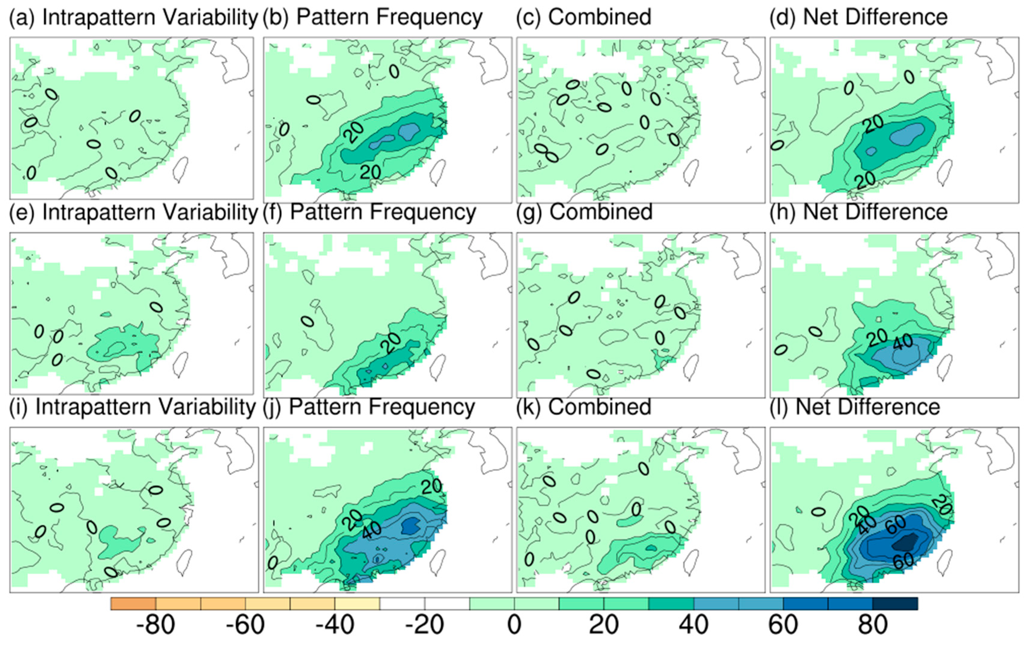
2.2.2. Attribution of Intraseasonal Precipitation Differences

Here, we follow the methodology from Schuenemann and Cassano [9], which was used to analyze the difference between each of the Intergovernmental Panel on Climate Change Fourth Assessment Report (IPCC AR4) models and ERA-40 reanalysis for the North Atlantic region. We present a new implementation of the method to define the relationship between precipitation days, precipitation intensity, and precipitation total for every grid point over southeastern China. For every grid point, the precipitation total ($P$) (mm) was calculated by multiplying the precipitation days ($f_n$) (day) by precipitation intensity ($p_n$) (mm/day).

$$P={\displaystyle \sum _{n=1}^{n\_WT}{f}_n{p}_n}$$

(3)

In order to investigate intraseasonal variation, the source of differences between different months in wintertime can be determined by rewriting Equation (3) as:

$$P={\displaystyle \sum _{n=1}^{n\_WT}(f_n+\Delta f_n)(p_n+\Delta p_n)}$$

(4)

Expanding the expression in Equation (4) gives:

$$P={\displaystyle \sum _{n=1}^{n\_WT}(f_n{p}_n+f_n\Delta p_n+\Delta f_n{p}_n+\Delta f_n\Delta p_n)}$$

(5)

which indicates that the total month precipitation of the latter can be represented as the former (first term), plus three terms that represent the net difference in month precipitation between the former and the latter.

The first difference term ($f_n\Delta p_n$) is referred to as the intra-pattern variability component. The different month may have different amounts of precipitation in the atmosphere or different precipitation physics, leading to the precipitation differences indicated by this term. The second difference term ($\Delta f_n{p}_n$) is the pattern frequency component. Therefore, this term represents the precipitation differences resulting from differences in the frequency of occurrence of synoptic patterns. The third difference term ($\Delta f_n\Delta p_n$) is referred to as the combined term. This part is often very small, so usually, only the first two items are discussed.

In this study, we found that precipitation was less in December and more in February. The attribution of intraseasonal variation of precipitation was made by following Schuenemann and Cassano [9]. This method allows a detailed look at what drives the differences between the two months on the synoptic scale. The advantages of this method are clear meaning and simple computation. In general, the change of WT itself will not be very obvious in the same season. However, this does not mean that the precipitation corresponding to each WT has not changed much. Since clustering is not based on precipitation data, we can only have a clear understanding of this by attribution analysis.

2.2.3. Calculation of the Teleconnection Patterns

Wallace and Gutzler [6] found that there are five teleconnection patterns at 500-hPa geopotential height anomalies over the winter northern hemisphere. These teleconnections include the eastern Atlantic pattern (EA), Pacific/North American pattern (PNA), western Atlantic pattern (WA), western Pacific pattern (WP), and Eurasian pattern (EU).

The teleconnection pattern indices of the front were defined as follows:

$$\mathrm{EA}=\frac{1}{2}{Z}^{*}(55{}^{\circ }\mathrm{N},20{}^{\circ }\mathrm{W})-\frac{1}{4}{Z}^{*}(25{}^{\circ }\mathrm{N},25{}^{\circ }\mathrm{W})-\frac{1}{4}{Z}^{*}(50{}^{\circ }\mathrm{N},40{}^{\circ }\mathrm{E})$$

(6)

$$\mathrm{PNA}=\frac{1}{4}[Z^{*}(20{}^{\circ }\mathrm{N},160{}^{\circ }\mathrm{W})-Z^{*}(45{}^{\circ }\mathrm{N},165{}^{\circ }\mathrm{W})+Z^{*}(55{}^{\circ }\mathrm{N},115{}^{\circ }\mathrm{W})-Z^{*}(30{}^{\circ }\mathrm{N},85{}^{\circ }\mathrm{W})]$$

(7)

$$\mathrm{WA}=\frac{1}{2}[Z^{*}(55{}^{\circ }\mathrm{N},55{}^{\circ }\mathrm{W})-Z^{*}(30{}^{\circ }\mathrm{N},55{}^{\circ }\mathrm{W})]$$

(8)

$$\mathrm{WP}=\frac{1}{2}[Z^{*}(60{}^{\circ }\mathrm{N},155{}^{\circ }\mathrm{E})-Z^{*}(30{}^{\circ }\mathrm{N},155{}^{\circ }\mathrm{E})]$$

(9)

$$\mathrm{EU}=-\frac{1}{4}{Z}^{*}(55{}^{\circ }\mathrm{N},20{}^{\circ }\mathrm{E})+\frac{1}{2}{Z}^{*}(55{}^{\circ }\mathrm{N},75{}^{\circ }\mathrm{E})-\frac{1}{4}{Z}^{*}(40{}^{\circ }\mathrm{N},145{}^{\circ }\mathrm{E})$$

(10)

where $Z^{*}$ is the normalized 500-hPa height anomalies at specified grid points corresponding to “centers of action” or antinodes of the pattern. Further details about the procedure for the calculation of the teleconnection indices can be found in Wallace and Gutzler [6].

3. Results

3.1. WTs

The k-means clustering algorithm is applied to NCEP-2 daily 850-hPa u and v component winds for the winter months of December–January–February (hereafter as DJF) 1979–2016 (standardized) within the region specified in Figure 1.

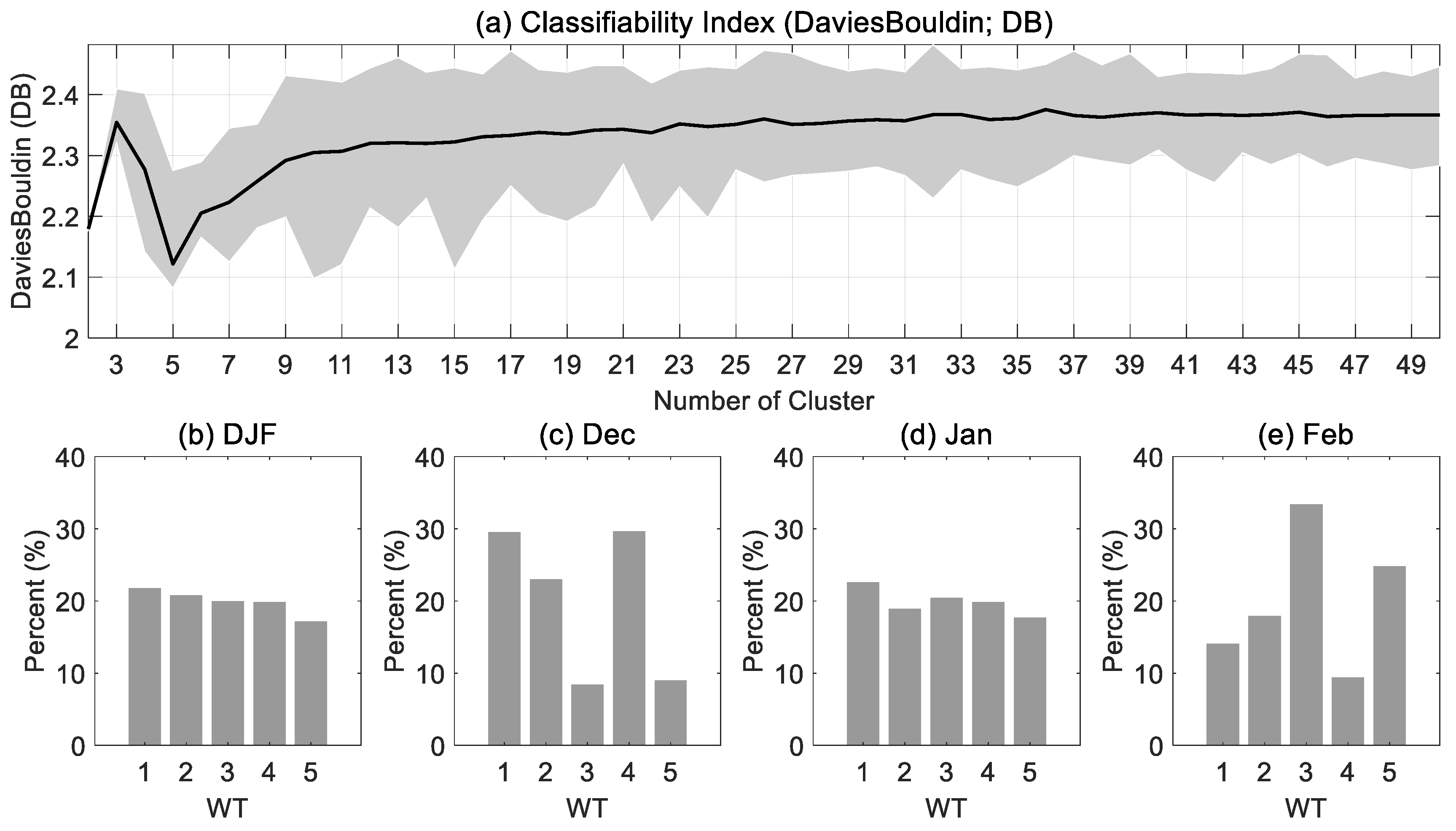
3.1.1. Determine the Optimal Number of Clusters

In order to ensure whether the clustering results have good reasonability to achieve adequate separation of the data, the optimal number of clusters k was determined by using the DB index in Figure 2a. The Monte Carlo simulation shows that the optimal number of clusters was five. In the following analysis, the 850-hPa winds will be separated into five distinct clusters using k-means clustering.

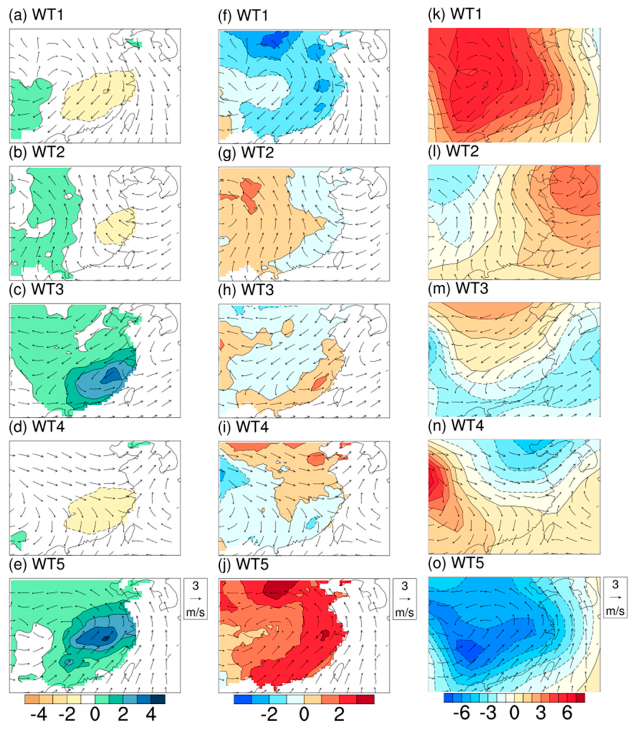
3.1.2. Occurrence Frequency and Spatial Distribution Characteristics of WTs

The next step is to analyze DJF WTs for southeastern China based on the five-cluster solution. Each WT is represented by a cluster. Each WT comprises ~17% to ~22% of the DJF days, with outbreak (WT1) having the greatest number of days (21.9%), and extinction (WT5) having the least number of days (17.3%) (Figure 2b). For the WTs of January (Figure 2d), the series of WT frequencies is similar to the series of WT frequencies in the entire DJF period (Figure 2b). While WT1, WT2, and WT4 are typically observed during December (Figure 2c), WT3 and WT5 mainly occur during February (Figure 2e). This suggests that there exist some strong intraseasonal frequency variations at the monthly scale for some WTs.

In order to have a clear understanding of the spatial distribution of each WT, we provide the five WTs over southeastern China in Figure 3. Compositions of 850-hPa wind anomalies and precipitation anomalies are shown in Figure 3a–e; wind anomalies and surface air temperature anomalies are shown in Figure 3f–j, and wind anomalies and sea level pressure anomalies are shown in Figure 3k–o.

In southeastern China, the precipitation anomalies are negative in WT1, WT2, and WT4 and positive in WT3 and WT5. WT1, with negative precipitation (Figure 3a) and negative temperature (Figure 3f), is characterized by a dry and cold climate. The East Asian winter monsoon is highly strong, and the continent is controlled by the high-pressure system (anticyclone) (Figure 3k). Due to the influence of northerly winds, it is difficult to form precipitation in southeastern China. A similar analysis shows that WT2 (Figure 3b,g,l) and WT4 (Figure 3d,i,n) are basically the same as WT1, but the formation mechanism behind them is different. WT2 is mainly caused by high pressure, while WT4 is mainly caused by prevailing northwest wind. In WT3 (Figure 3c,h,m), precipitation is also prone to occur in southeastern China. The northern part of the continent is controlled by cold high pressure, and the southern part of the continent is controlled by warm low pressure (Figure 3m). The dry and cold air flow meets the warm and wet airflow in the southeastern region, which is favorable for the formation of precipitation. WT5 (Figure 3e,j,o) is characterized by a warm humid climate. Not only are the anomalies of precipitation positive, but the anomalies of temperature are positive, too. The East Asian winter monsoon is obviously weaker, and the continent is controlled by the low-pressure system (cyclone). Strong low-level southerly flow brings warm moisture to southeastern China, and is conducive to the formation of heavy rainfall in southeastern China.

These results imply that the formation mechanisms of WT1, WT2, and WT4 are different, although they are all characterized by negative anomalies of precipitation. WT1 and WT2 are all controlled by high pressure. Although there is moisture, it is difficult to form precipitation due to subsidence. Unlike WT1 and WT2, the reason why WT4 is difficult to form precipitation is the prevailing northwest wind, which does not bring moisture. Similarly, although WT3 and WT5 exhibit positive anomalies in precipitation, their formation mechanisms are different. Precipitation in WT3 is caused by the confluence of dry cold air flow and warm humid air flow. Unlike WT3, precipitation in WT5 is caused by sufficient moisture and updraft.

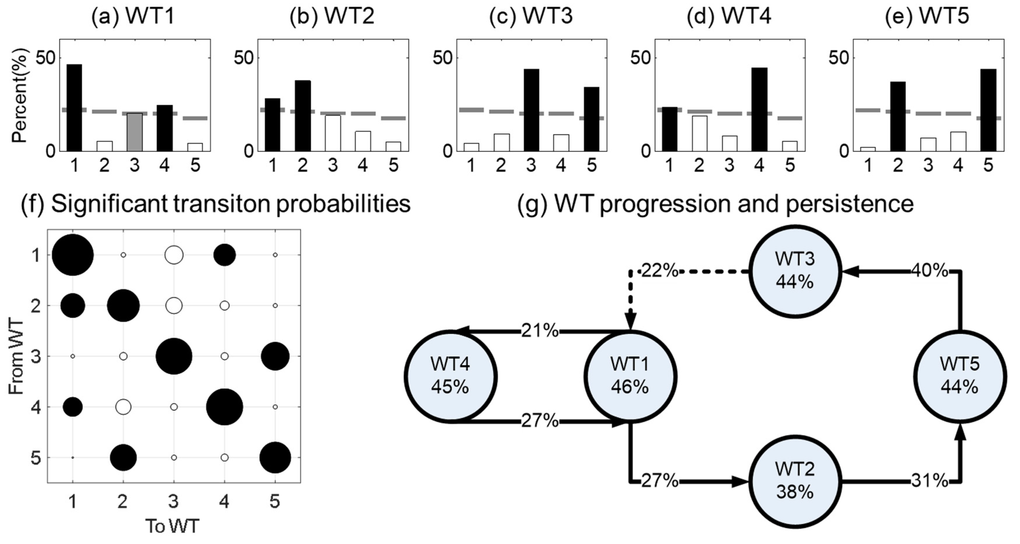
3.2. Progression and Persistence of WTs

While identifying WTs of daily 850-hPa winds provides the characteristic weather patterns over southeastern China, more information on WTs is given in the rule of remaining in the original WT (persistence) or switching to a new WT (progression) on the following day [3]. The statistical results should help us to understand more about how often a particular WT transitions to each of the other WTs [26].

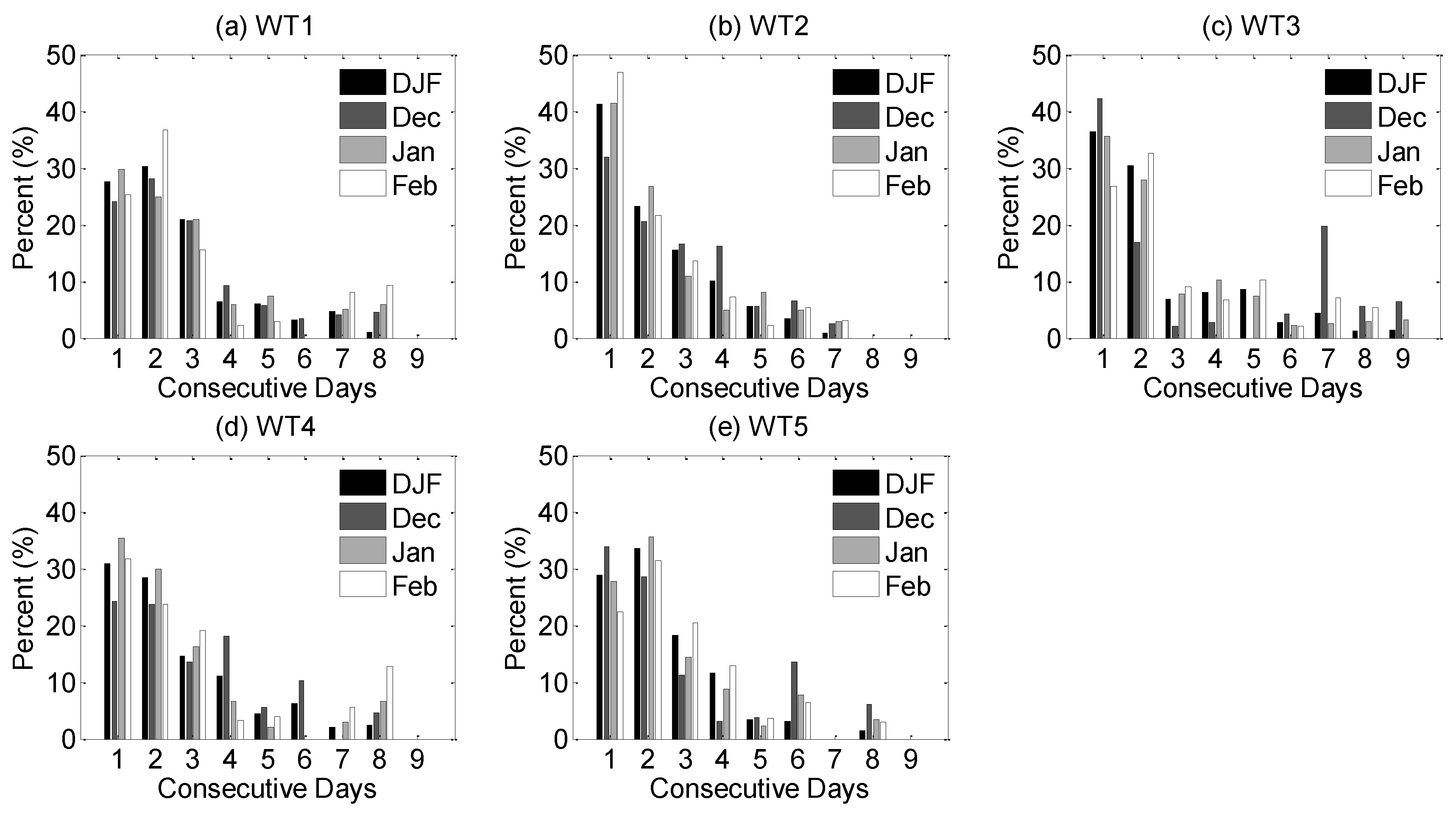
3.2.1. WT Persistence

In Figure 4, we plot the duration in the DJF season for each WT. About 27.5–41.2% of DJF days persist in the same WT for one day. The mean duration for each WT ranges from 1.60 days for WT2 to 1.86 days for WT1, and there are somewhat intraseasonal duration variations at the monthly scale. While longer duration for WT3 or WT5 is typically observed during December, the longer duration for WT1 or WT4 is typically observed during February. On the contrary, WT2 shows almost constant duration, and its duration is the shortest of all the WTs.

An analysis of spell lengths (not shown in Figure 4) shows that larger duration differences exist between different WTs. For spells lasting longer than five days, WT1 rose from 17.8% for December to 20.1% for February, and WT4 rose from 20.3% for December to 22.2% for February. On the contrary, WT3 fell from 35.9% for December to 24.7% for February, and WT5 fell from 23.3% for December to 12.9% for February. For spells lasting longer than seven days, this duration difference is more obvious. WT1 rose from 8.6% for December to 17.2% for February, and WT4 rose from 4.5% for December to 18.3% for February. On the contrary, WT3 fell from 31.7% for December to 6.0% for February, and WT5 fell from 12.5% for December to 2.9% for February. The change in WT2 is not obvious.

3.2.2. WT Progression

Besides self-transitions, the persistence mentioned above, which has a progression that is helpful for us to make clear how often a particular WT progresses to each of the other WTs [26], needs to be counted. Next, we illustrate the progression of each WT in Figure 5a–g. Following the approach in Roller et al. [3], the 95% confidence interval of the WT distribution on the following days is determined by randomly sampling a number of days in the 38-year record equal to each WT count, calculating the distribution of the following day WTs for each sample, and repeating the process 1000 times. The percentages that are higher (lower) than the top 97.5% (bottom 2.5%) indicate a transition to a WT that is more (less) likely than that due to chance, and is shown as black (white) bars. The following day is shown in Figure 5a–e respectively.

Significant probability transitions from one WT to another one are illustrated in Figure 5f. The horizontal axis represents the type that the WT will convert to the next day. The vertical axis represents the type converted from the previous day. The size of the circle on the diagonal represents the percentage of persistence in themselves. As shown in the figure, we find that each WT has great inertia of self-preservation. Their conversion to other types is not high (some are even close to zero).

Figure 5g shows the likelihood (expressed as a percentage of times) that a WT persists or transitions. All the WTs are most likely to persist as themselves. The respective percentage of persistence is 46%, 38%, 44%, 45%, and 44%. WT1 and WT4 are most likely to progress to each other. At the same time, WT1 also forms a chain with other WTs in progress. The sequence of the chain is WT1, WT2, WT5, WT3, and WT1. In particular, the chain of WTs that we have found (i.e., WT1→WT2→WT5→WT3→WT1) should be focused on a bit more, referring to the spatial patterns of WTs. Based on the statistic analysis, we found that the chain has appeared 21 times in 1979–2016 (38 years). It can be understood as a dynamical process of a large-scale strong cold air invasion into China southward, which drives the chains. This process can be understood as several stages, such as gestation (WT3), outbreak (WT1), eastward withdrawal (WT2), and extinction (WT5).

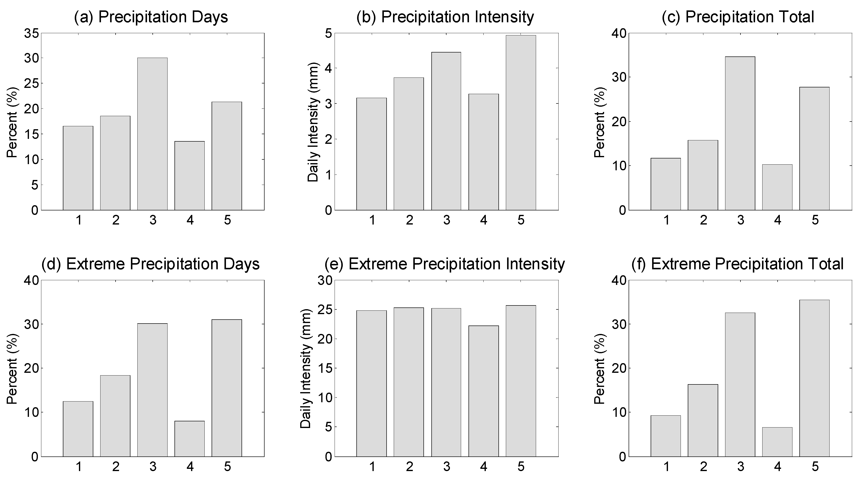
3.3. Relationships between WTs and Precipitation

3.3.1. Characteristics of Precipitation and Extreme Precipitation

Are the WTs related to near-surface climate variability such as precipitation? In the following section, we address this question by examining whether the daily precipitation (precipitation over 0.254 mm, or 0.01 inch) and extreme precipitation (defined as the top 1% of daily intensity on days with precipitation) associated with the WTs. The results of DJF mean are presented in Figure 6.

Based on the CHEN05 daily precipitation data, it is clear that the number of precipitation days and precipitation intensity differs between WTs. Most precipitation days occur in WT3 and WT5. The intensity of precipitation is the highest in WT5, followed by WT3. The most extreme precipitation occurs in WT3 and WT5. The extreme precipitation intensity is the highest in WT5. For WT3 and WT5, their total precipitation and total extreme precipitation are the highest of all the WTs.

Although precipitation and extreme precipitation can occur in every WT (Figure 6), they are more likely to occur in WT3 and WT5, and are less likely to occur in WT1, WT2, and WT4. The reason is that WT3 and WT5 are conducive to the formation of all conditions for the formation of winter precipitation. Conditions are as follows: unusual southerly winds, sufficient vapor, the confluence of cold and warm air masses, and large-scale airflow uplift [27].

3.3.2. Attribution of Intraseasonal Precipitation Differences

In order to have a detailed look at what drives the intraseasonal precipitation differences in the wintertime season (DJF), the partitioning (Equation (5)) of the intraseasonal precipitation differences between each pair of the three months making up the wintertime season (DJF) were performed. Figure 7 illustrates the calculation results.

The pattern frequency component is predominantly responsible for the intraseasonal precipitation differences (Figure 7b,f,j). In other words, the main reason is that the frequencies of WTs vary in different months. In different months of the same season, precipitable water in the atmosphere or precipitation physics is similar. The intra-pattern variability component and the combined term in the intraseasonal precipitation differences only play a small role (Figure 7a,e,i).

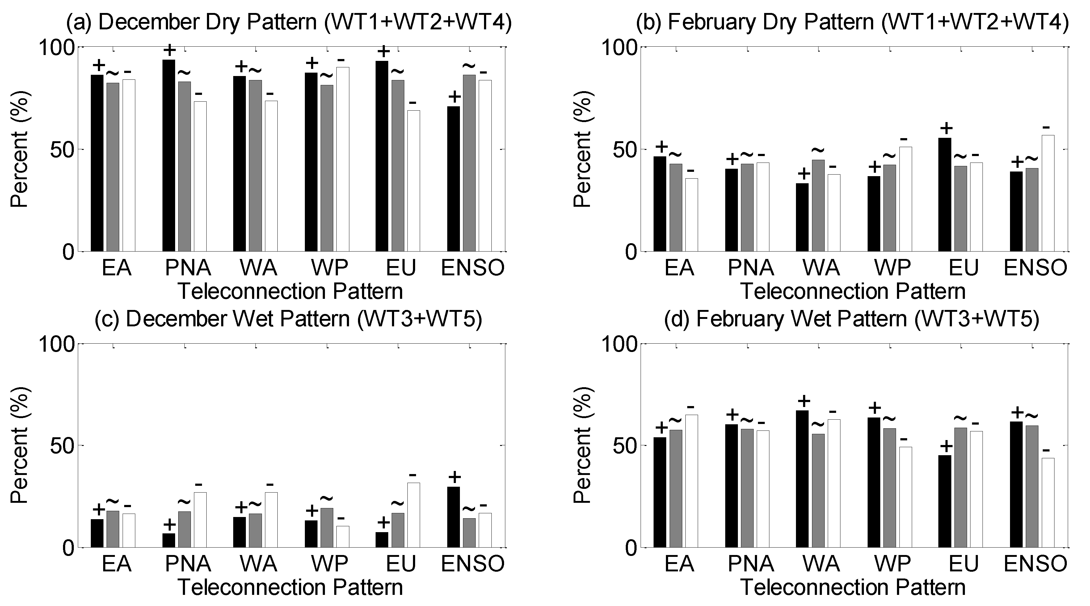
3.4. Relationships between WTs and Teleconnections

Following Roller et al. [3], the relative frequency of WT for each teleconnection phase was determined in our analysis. We are more concerned about the precipitation related WTs and their intraseasonal variations. Thus, we present a new implementation according to the relationship between each WT and precipitation. WTs were regrouped into two broad categories, which are called dry WTs (WT1 + WT2 + WT4) and wet WTs (WT3 + WT5). The frequencies of dry WTs and wet WTs in December and February were counted respectively (Figure 8).

There is a large intraseasonal variation of frequencies for all teleconnection patterns. The frequencies of dry patterns were higher in December (Figure 8a) and lower in February (Figure 8b). On the contrary, the frequencies of wet patterns were low in December (Figure 8c) and increased in February (Figure 8d). During the positive phase (>1) of the EA, PNA, WA, and EU, the neutral phase (≥−1 and ≤1) of the ENSO, and the negative phase (<−1) of the WP, the likelihood of dry patterns increased in December (Figure 8a). During the positive phase (>1) of the EA and EU, the neutral phase (≥−1 and ≤1) of the WA, and the negative phase (<−1) of the PNA, WP, and ENSO, the likelihood of dry patterns increased in February (Figure 8b). During the positive phase (>1) of the ENSO, the neutral phase (≥−1 and ≤1) of the EA and WP, and the negative phase (<−1) of the PNA, WA, and EU, the likelihood of wet patterns increased in December (Figure 8c). During the positive phase (>1) of the PNA, WA, WP, and ENSO, the neutral phase (≥−1 and ≤1) of the EU, and the negative phase (<−1) of the EA, the likelihood of wet patterns increased in February (Figure 8d).

Table 1. The links to the various teleconnection phases (positive or negative), the variation of frequencies of different WTs (Dry and Wet), and the correlation to higher or lower amounts of precipitation. The bold font marks types that play leading roles. EA: eastern Atlantic pattern, PNA: Pacific/North American pattern, WA: western Atlantic pattern, WP: western Pacific pattern, and EU: Eurasian pattern, ENSO: El Niño–Southern Oscillation.

Category	EA	PNA	WA	WP	EU	ENSO	Frequency	Precipitation
Dec_ Dry (WT1 + WT2 + WT4)	+	+	+	−	+	−	↑	↓
Feb_ Dry (WT1 + WT2 + WT4)	+	−	−	−	+	−	↓	↓
Dec_ Wet (WT3 + WT5)	−	−	−	+	−	+	↓	↑
Feb_ Wet (WT3 + WT5)	−	+	+	+	−	+	↑	↑

summarized the results. Dry patterns (WT1 + WT2 + WT4) and wet patterns (WT3 + WT5) play leading roles in December and February, respectively. In December, less precipitation was due to the higher frequencies of dry patterns and lower frequencies of wet patterns. Ignoring the middle phase, the positive and negative phases are contrasted here. It is often accompanied by the positive phase of EA, PNA, WA, and EU, and the negative phase of WP and ENSO. In February, less precipitation was due to the higher frequencies of wet patterns and lower frequencies of dry patterns. It is often accompanied by the positive phase of PNA, WA, WP, and ENSO, and the negative phase of EA and EU.

Therefore, it suggested that except for PNA and WA, the other four teleconnection patterns (EA, WP, EU, and ENSO) are closely related to the WTs that are closely related to precipitation. During the positive phase of the WP and ENSO and the negative phase of the EA and EU, the likelihood of wet patterns will increase. On the contrary, during the positive phase of the EA and EU and the negative phase of the WP and ENSO, the likelihood of dry patterns will increase. Given that PNA and WA occur far away from southeastern China, it is easily expected that they are not related to the WTs. The main mechanism of EA affecting winter climate in China is similar to the EU. They are mainly due to the interaction of the anticyclonic circulation anomalies in Siberia and the two cyclonic circulation anomalies near the Bay of Bengal and northeast China. In a positive anomaly, the circulation structure promotes the southward movement of cold air, while in a negative anomaly, the opposite is true.

In addition to the above teleconnection, MJO also plays an important role in the evolution of weather and climate, and the intensity of MJO in winter is stronger than that in summer [8]. In order to understand the influence of MJO on winter precipitation in southeastern China, the relative frequencies of WTs corresponding to eight different MJO phases were calculated separately (Figure 9).

In December (Figure 9a), during the strong state of MJO (denoted by H) for dry patterns, the likehood of the sixth, seventh, and eighth phase increases, while the likehood of the first, second, and third phase decreases. During the weak state of MJO (expressed as L), the opposite is true. For wet patterns (Figure 9c), the situation is opposite to the corresponding dry patterns (Figure 9a). This result implies that the first, second, and third phases of MJO are beneficial to the occurrence of winter precipitation in southeastern China in December, while the sixth, seventh, and eighth phases of MJO have inhibitory effects on precipitation. In February (Figure 9b), during the strong state of MJO for dry patterns, the likehood of the fifth, sixth, and seventh phase increases, while the likehood of the second, third, and eighth phase decreases. During the weak state of MJO (expressed as L), the opposite is true. For wet patterns (Figure 9d), the situation is opposite to the corresponding dry patterns (Figure 9b). This result implies that the second, third, and eighth phases of MJO are beneficial to precipitation, while the fifth, sixth, and seventh phases of MJO have inhibitory effects on precipitation.

Our findings are in agreement with Jia et al. [28] that the phase change of MJO has considerable influence on winter rainfall in China [28]. Influenced by the phase change of MJO, changes have taken place in the southern trough of the Bay of Bengal and the western Pacific subtropical high, which ultimately led to changes of northward moisture transport coming from the Bay of Bengal and the South China Sea.

4. Discussion

Getting more acquainted with the precipitation associated with the WTs, WTs were reassembled and named as two different types: dry pattern and wet pattern. To understand the roles that teleconnections play in wintertime weather over southeastern China, the dry pattern and wet pattern frequencies during various phases of the teleconnections were counted. Moreover, statistics and comparisons of the difference of relationship between the teleconnection phases and dry pattern and wet pattern during December and February were also carried out. However, our analytical methods and computational results differ from previous studies [3,4]. The characteristic of our analysis is to recombine the categories that are prone and not prone to precipitation. As mentioned in Roller et al. [3], it is possible that switching from one WT to another is associated with some kind of teleconnection phase switching from positive/negative to negative/positive.

In particular, we find a distinct evolutionary chain in the analysis of the rule of pattern evolution (WT3→WT1→WT2→WT5→WT3). The chain corresponds to some specific stages of cold air activity (gestation (WT3), outbreak (WT1), eastward withdrawal (WT2), and extinction (WT5)). Over the past 38 years (1979–2016), the chain has appeared frequently (21 times). This result fully illustrates that the physical process of cold air activity in winter can be captured by the progression rule of wet and dry patterns. In addition, WT1 indicates that the whole area is controlled by an anticyclone, resulting in a dry and cold climate throughout the whole area. Unlike WT1, WT4 is explained by the prevailing northwest wind caused by a trough, which leads to dry and cold weather. WT1 and WT4 weather patterns are similar, but the physical processes behind them are quite different. The transition between them is just the transition between these two physical states.

5. Conclusions

In this paper, the frequency, persistence, and progression of different WTs in southeastern China and their relationship with precipitation and teleconnection were analyzed. The causes of intraseasonal differences in precipitation were analyzed. These analyses lay a foundation for our understanding of the relationship between large-scale circulation and local weather patterns. Based on this, the physical mechanism of winter precipitation and its intraseasonal variation in southeastern China under the influence of large-scale circulation are revealed. The main conclusions are as follows:

(1) The DB index can be used to determine the best optimal WTs (the optimal number of WTs is five). Whether the number of WTs can be reasonably chosen determines whether the analysis of the evolution of WT is correct or not. WTs obtained by the k-means clustering analysis can provide an objective categorization and consider all days. With these WTs, we can identify which ones are most likely to generate precipitation.

(2) Different WTs may have similar precipitation patterns, which can be classified as dry and wet on the whole. The precipitation anomalies of WT1, WT2, and WT4 are negative, while those of WT3 and WT5 are positive. However, the precipitation caused by different WTs has totally different formation mechanisms. These differences can be effectively identified by the k-means clustering analysis method.

(3) In the analysis of the evolution of WT, we find a special evolutionary chain that can be used to explain the cold wave weather process in winter. The sequence of the chain is WT3→WT1→WT2→WT5→WT3. The different stages of the cold wave weather process correspond to the different WTs in the evolutionary chain, and can well correspond to the teleconnection phase changes. The special phases of EA, WP, EU, ENSO, and MJO also correspond to them.

(4) Precipitation in December and February is quite different. Then, the intraseasonal differences of precipitation were decomposed into three different parts: the intra-pattern variability component, the pattern frequency component, and the combined term. The intraseasonal variation of precipitation can be attributed to the intraseasonal variation of the frequency of WT occurrence. In December, dry modes such as WT1, WT2, and WT4 appeared more frequently, while wet modes such as WT3 and WT5 appeared more frequently in February.

Our work establishes a link between synoptic-scale and large-scale circulation, thus providing a reference for climate model simulation and future climate prediction.

References

1. Wang, L.; Cao, G.; Zhang, Q.; Sun, J.; Wang, Z.; Zhang, Y.; Zhao, S.; Chen, X.; Chen, Y. Analysis of the severe cold Surge, ice-snow and frozen disasters in South China during January 2008: I. Climatic features and its impacts. Meteorol. Mon. 2008, 34, 95–100. (In Chinese) [Google Scholar]
2. Gao, H.; Chen, L.; Jia, X.; Ke, Z.; Han, R.; Zhang, P.; Wang, Q.; Sun, C.; Zhu, Y.; Li, W.; et al. Analysis of the severe cold surge, ice-snow and frozen disasters in south China during January 2008: II. Possible climatic causes. Meteorol. Mon. 2008, 34, 101–106. (In Chinese) [Google Scholar]
3. Roller, C.D.; Qian, J.; Agel, L.; Barlow, M.; Moron, V. Winter weather regimes in the Northeast United States. J. Clim. 2016, 29, 2963–2980. [Google Scholar] [CrossRef]
4. Gerlitz, L.; Steirou, E.; Schneider, C.; Moron, V.; Vorogushyn, S.; Merz, B. Variability of the cold season climate in Central Asia-Part I: Weather types and their tropical and extratropical drivers. J. Clim. 2018, 31, 7185–7207. [Google Scholar] [CrossRef]
5. Davies, D.L.; Bouldin, D.W. A cluster separation measure. IEEE Comput. Soc. 1979, 1, 224–227. [Google Scholar] [CrossRef]
6. Wallace, J.M.; Gutzler, D.S. Teleconnections in the geopotential height field during the Northern Hemisphere winter. Mon. Weather Rev. 1981, 109, 784–812. [Google Scholar] [CrossRef]
7. Kiladis, G.N.; Diaz, H. Global climatic anomalies associated with extremes in the Southern Oscillation. J. Clim. 1989, 2, 1069–1090. [Google Scholar] [CrossRef]
8. Madden, R.A.; Julian, P.R. Observations of the 40–50-Day Tropical Oscillation—A Review. Mon. Weather Rev. 1994, 122, 814–837. [Google Scholar] [CrossRef] [Green Version]
9. Schuenemann, K.C.; Cassano, J.J. Changes in synoptic weather patterns and Greenland precipitation in the 20th and 21st centuries: 1. Evaluation of late 20th century simulations from IPCC models. J. Geophys. Res. 2009, 114. [Google Scholar] [CrossRef] [Green Version]
10. Kanamitsu, M.; Ebisuzaki, W.; Woollen, J.; Yang, S.; Hnilo, J.J.; Fiorino, M.; Potter, G.L. NCEP–DOE AMIP-II Reanalysis (R-2). Bull. Am. Meteorol. Soc. 2002, 83, 1631–1643. [Google Scholar] [CrossRef]
11. Chen, D.; Ou, T.; Gong, L.; Xu, C.; Li, W.; Ho, C.H.; Qian, W. Spatial interpolation of daily precipitation in China: 1951–2005. Adv. Atmos. Sci. 2010, 27, 1221–1232. [Google Scholar] [CrossRef]
12. Reynolds, R.W.; Rayner, N.A.; Smith, T.M.; Stokes, D.C.; Wang, W. An improved in situ and satellite SST analysis for climate. J. Clim. 2002, 15, 1609–1625. [Google Scholar] [CrossRef]
13. Wheeler, M.C.; Hendon, H.H. An all-season real-time multivariate MJO Index: Development of an index for monitoring and prediction. Mon. Weather Rev. 2004, 132, 1917–1932. [Google Scholar] [CrossRef]
14. Xu, Y.; Gao, X.; Shen, Y.; Xu, C.; Shi, Y.; Giorgi, F. A Daily Temperature Dataset over China and Its Application in Validating a RCM Simulation. Adv. Atmos. Sci. 2009, 26, 763–772. [Google Scholar] [CrossRef]
15. Diday, E.; Simon, J.C. Clustering analysis. In Digital Pattern Recognition; Springer: Berlin, Germany, 1976; pp. 47–94. [Google Scholar]
16. Ghil, M.; Robertson, A.W. “Waves” vs. “particles” in the atmosphere’s phase space: A pathway to long-range forecasting? Proc. Natl. Acad. Sci. USA 2002, 99, 2493–2500. [Google Scholar] [CrossRef]
17. Straus, D.M.; Corti, S.; Molteni, F. Circulation Regimes: Chaotic Variability versus SST-Forced Predictability. J. Clim. 2007, 20, 2251–2272. [Google Scholar] [CrossRef]
18. Moron, V.; Robertson, A.W.; Qian, J. Local versus regional-scale characteristics of monsoon onset and post-onset rainfall over Indonesia. Clim. Dyn. 2010, 34, 281–299. [Google Scholar] [CrossRef]
19. Qian, J.H.; Robertson, A.W.; Moron, V. Interactions among ENSO, the Monsoon, and Diurnal Cycle in Rainfall Variability over Java, Indonesia. J. Atmos. Sci. 2010, 67, 3509–3524. [Google Scholar] [CrossRef]
20. Conway, D.; Jones, P.D. The use of weather types and air flow indices for GCM downscaling. J. Hydrol. 1998, 212, 348–361. [Google Scholar] [CrossRef]
21. Moron, V.; Robertson, A.W.; Ward, M.N.; Ndiaye, O. Weather Types and Rainfall over Senegal. Part I: Observational Analysis. J. Clim. 2008, 21, 266–287. [Google Scholar] [CrossRef]
22. Demuzere, M.; Werner, M.; van Lipzig, N.P.M.; Roeckner, E. An analysis of present and future ECHAM5 pressure fields using a classification of circulation patterns. Int. J. Climatol. 2009, 29, 1796–1810. [Google Scholar] [CrossRef] [Green Version]
23. Riddle, E.E.; Stoner, M.B.; Johnson, N.C.L.; Heureux, M.L.; Collins, D.C.; Feldstein, S.B. The impact of the MJO on clusters of wintertime circulation anomalies over the North American region. Clim. Dyn. 2012, 40, 1749–1766. [Google Scholar] [CrossRef] [Green Version]
24. Perez, J.; Menendez, M.; Mendez, F.J.; Losada, I.J. Evaluating the performance of CMIP3 and CMIP5 global climate models over the north-east Atlantic region. Clim. Dyn. 2014, 43, 2663–2680. [Google Scholar] [CrossRef]
25. Michelangeli, P.A.; Vautard, R.; Legras, B. Weather regimes: Recurrence and quasi stationarity. J. Atmos. Sci. 1995, 52, 1237–1256. [Google Scholar] [CrossRef]
26. Coleman, J.S.M.; Rogers, J.C. A Synoptic Climatology of the Central United States and Associations with Pacific Teleconnection Pattern Frequency. J. Clim. 2007, 20, 3485–3497. [Google Scholar] [CrossRef]
27. Zhang, Z.; Gong, D.; Hu, M.; Guo, D.; He, X.; Lei, Y. Anomalous Winter Temperature and Precipitation Events in Southern China. J. Geogr. Sci. 2009, 19, 471–488. [Google Scholar] [CrossRef]
28. Jia, X.; Chen, L.; Ren, F.; Li, C. Impacts of the MJO on winter rainfall and circulation in China. Adv. Atmos. Sci. 2011, 28, 521–533. [Google Scholar] [CrossRef]
Figure 1. Analysis domain: the boundaries (small rectangle) of the southeast region (covering southeastern China) used to subset NCEP2 850-hPa winds for input to the k-means clustering algorithm.
Atmosphere 10 00271 g001
Figure 2. The classifiability index (BDs) results from the k-means clustering of two to 50 clusters (black line) and the 100 repeated calculation results (gray range). The figure shows the (a) optimal number of clusters (BD for various numbers of clusters) and percent of days assigned to each clustered weather type (WT) for (b) the entire winter season (December–February) and for (c) December, (d) January, and (e) February. BD: Davies–Bouldin.
Atmosphere 10 00271 g002
Figure 3. (Left column) NCEP-DOE reanalysis II (NCEP-2) 850-hPa wind anomalies for December–January–February (DJF) 1979–2016 (vectors) and the CHEN05 precipitation anomalies for DJF 1979–2005 (shaded; mm/day) for (a) WT1, (b) WT2, (c) WT3, (d) WT4, and (e) WT5. (middle column) NCEP2 850-hPa winds anomalies for DJF 1979–2016 (vectors) and the CN05 surface air temperature anomalies for DJF 1979–2005 (shaded; °C) for (f) WT1, (g) WT2, (h) WT3, (i) WT4, and (j) WT5. (right column) NCEP2 850-hPa winds anomalies for DJF 1979–2016 (vectors) and the sea-level pressure anomalies for DJF 1979–2016 (shaded; hPa) for (k) WT1, (l) WT2, (m) WT3, (n) WT4, and (o) WT5.
Atmosphere 10 00271 g003
Figure 4. WT persistence, expressed as a percentage of total WT days, for duration of one to nine days.
Atmosphere 10 00271 g004
Figure 5. Progression of each WT, shown as frequency of WTs both on days following (a) WT1, (b) WT2, (c) WT3, (d) WT4, and (e) WT5 days. The distribution on the next day and the previous day is shown in the first and second rows, respectively. Significant and not significant conversions are shown with black bars and white bars, respectively. (f) Significant probability transitions from one WT to another one. (g) Graphical representation of WT progression and persistence. Significant and not significant conversions are represented by solid arrows and dotted arrows, respectively.
Atmosphere 10 00271 g005
Figure 6. Mean precipitation characteristics of CHEN05 for December–January–February (DJF) 1979-2005. (a) The number of precipitation days (expressed as a percentage of all precipitation days) for each WT. (b) The mean daily precipitation intensity (mm/day) for each WT. (c) The mean total precipitation (%) for each WT. (df) Precipitation days, intensity, and totals for extreme precipitation, defined as the top 1% of precipitation daily intensity.
Atmosphere 10 00271 g006
Figure 7. (top row) Differences between December and January. (middle row) Differences between January and February. (bottom row) Differences between December and February. The three columns on the left side of each row are the three difference terms: the intra-pattern variability component, the pattern frequency component, and the combined term. The right side of each row is the total difference.
Atmosphere 10 00271 g007
Figure 8. Intraseasonal variation of frequencies of different WTs (Dry and Wet). Frequencies for (a) December Dry Pattern (WT1 + WT2 + WT4), (b) February Dry Pattern (WT1 + WT2 + WT4), (c) December Wet Pattern (WT3 + WT5), and (d) February Wet Pattern (WT3 + WT5) during various phases of the teleconnection patterns. For each teleconnection pattern, the three bars represent the positive (+), neutral (~), and negative (−) phases.
Atmosphere 10 00271 g008
Figure 9. Intraseasonal variation of frequencies of different WTs (Dry and Wet). Frequencies for (a) December Dry Pattern (WT1 + WT2 + WT4), (b) February Dry Pattern (WT1 + WT2 + WT4), (c) December Wet Pattern (WT3 + WT5), and (d) February Wet Pattern (WT3 + WT5) during eight different phases of Madden–Julian Oscillation (MJO). For each MJO phase, the two bars represent the strong (denoted by H) MJO and weak (expressed as L) MJO, respectively.
Atmosphere 10 00271 g009