Article

The Linkage of the Large-Scale Circulation Pattern to a Long-Lived Heatwave over Mideastern China in 2018

Key Laboratory of Regional Climate-Environment for Temperate East Asia, Institute of Atmospheric Physics, Chinese Academy of Sciences and University of Chinese Academy of Sciences, Beijing 100029, China
*
Author to whom correspondence should be addressed.
Atmosphere 2019, 10(2), 89; https://doi.org/10.3390/atmos10020089
Submission received: 30 January 2019 / Revised: 14 February 2019 / Accepted: 16 February 2019 / Published: 20 February 2019

Abstract

:
In this study, the large-scale circulation patterns (a blocking high, wave trains and the western Pacific subtropical high (WPSH)) associated with a wide ranging and highly intense long-lived heatwave in China during the summer of 2018 are examined using both observational data and reanalysis data. Four hot periods are extracted from the heatwave and these are related to anticyclones (hereafter referred to as heatwave anticyclone) over the hot region. Further analysis shows a relationship between the heatwave anticyclone and a synthesis of low, mid- and high latitude circulation systems. In the mid-high latitudes, a midlatitude wave train and a high latitude wave train are associated with a relay process which maintains the heatwave anticyclone. The midlatitude wave train acts during 16–21 July, whereas the high latitude wave train takes affect during 22–28 July. The transition between the two wave trains leads to the northward movement of the hot region. With the help of a wave flux analysis, it was found that both wave trains originate from the positive North Atlantic Oscillation (NAO+) which acts as an Atlantic wave source. Serving as a circulation background, the blocking situated over the Scandinavia-Ural sector is maintained for 18 days from 14 to 15 August, which is accompanied by the persistent wave trains and the heatwave anticyclone. Additionally, the abnormal northward movement of the WPSH and its combination with the high latitude wave train lead to the occurrence of extreme hot weather in north-eastern China occurring during the summer of 2018.

1. Introduction

Under a global warming background, more heatwaves with stronger intensities and longer durations are being observed around the world [1,2], including across China [3,4,5,6,7,8]. For instance, the trend in heatwaves defined by a percentile threshold in eastern China is positive during the 1979–2010 period [9], especially since eastern China has experienced an increased occurrence of rapid warming and heatwave days following the 1990s [10]. Recently, more studies have been conducted, which focus on the factors that cause heatwaves, as heatwaves can lead to disastrous damages to human health, society and ecosystems [11,12,13,14]. Examples of disastrous heatwaves include the European heatwave in 2003 [15] and the Russian heatwave in 2010 [16,17,18]. A severe heatwave occurred in eastern China in the summer of 2013. During this heatwave, humans, livestock and crops suffered from severe water shortages [19] and the accompanying drought resulted in direct economic losses of approximately 59 billion RMB [10]. Another high impact event was the heatwave in 2017 over northern and eastern China, where temperatures at many stations broke historical records. Among the record-breaking stations, the Xujiahui station had the highest temperature of 40.9 °C since 1873 [20]. This heatwave led to overloaded power grids in many provinces and the heat stress caused crops to burn and increased aquatic product mortality [21].
Following the 2017 summer heatwave, mideastern China experienced an excessively long heatwave over a wide-ranging area in the summer of 2018, which was sustained for 33 days from 17 July to 15 August, resulting in record-breaking overloaded power grids in many areas (China Meteorological Administration, 2018). On 20 July, the total area with temperatures above 35 °C reached 1,598,000 km2, involving 18 provinces (cities or districts), while 38 °C was identified over a total area of 134,000 km2. In the Liaoning Province (123.38° E, 41.80° N, Figure 1), the hot weather has had the longest duration, widest range and strongest intensity between 28 July and 4 August since 1951. The daily maximum temperature broke historical records at more than half of the national meteorological observation stations. The Jilin Province (125.35° E, 43.88° N, Figure 1) had a 16-day wide-ranging period of hot weather, which is historically quite rare. In addition, Japan and the Korean Peninsula also experienced high temperatures. Japan set a national temperature record of 41.1 °C on 23 July in Kumagaya, Saitama (Japan Meteorological Agency, 2018) and South Korea had an all-time high temperature record of 40.7 °C on 1 August in Hongcheon, Gangwon Province (Korea Meteorological Administration, 2018). Simultaneously, high temperatures were also observed in Northern Europe. The heatwave in Scandinavia included temperatures that topped 30 °C inside the Arctic Circle. In addition, Norway had a record temperature of 33.5 °C in Badufoss on 17 July and Finland also experienced a temperature of 33.4 °C in Kevo (WMO, 2018).
As has been studied previously, heatwaves are typically accompanied by an anomalous anticyclone [22,23]. In the higher latitudes, the anticyclone is recognized as a blocking high, whose persistence often leads to extreme weathers such as heatwaves, droughts and floods in summer [24,25,26,27,28]. For instance, a blocking anticyclone was the most important circulation system for the Russian heatwave in the summer of 2010 [16] and the 2003 European heatwave was also dominated by a persistent blocking high [29]. Blocking anticyclones favour land surface warming by enhancing adiabatic heating through increased subsidence and insolation due to fewer clouds [30]. In the midlatitudes, the quasi-stationary wave trains are linked to severe extreme weather events. Midlatitude synoptic waves that are trapped within midlatitude waveguides of free waves with the same wavenumbers can become quasi-resonant and cause heatwaves [31]. Ding and Wang [32] revealed that the circumglobal teleconnection (CGT) is characterized by rainfall and temperature anomalies in some midlatitude continental regions. Hong et al. [33] found that the Silk Road Pattern, which is a wave train along the Asian jet that occurs in summer, can modulate heatwaves in the midlatitudes of Eurasia. Heatwaves in lower latitudes are usually associated with a subtropical high. The mega-heatwave that occurred in Europe in July 2017 is characterized by a long-lasting subtropical high that favours the transport of warm air masses from the south [34]. In southern China, heatwaves often occur when the West Pacific Subtropical High (WPSH) extends westward and intensifies [35].
The heatwave in the summer of 2018 has a duration of 33 days, which can be treated as an intraseasonal event. The long duration of the heatwave is difficult to be explained by only one large-scale circulation process, because atmospheric circulation systems can have time-scales less than 10 days [36]. Thus, it motivates us to analyse if the heatwave is associated with different circulation processes and interactions of those. Through composite analyses of four periods during the heatwave, we will see that a midlatitude wave train, a high latitude wave train and the northward movement of the WPSH are the three dominant circulation patterns. However, different circulation patterns take effect at different time periods of the long-lived heatwave. Thus, it is essential to investigate the characteristics of these circulations and determine their sequential order, which can help us to better understand the formation mechanisms of the heatwave.
The article is organized as follows: the data and methods used in this paper are described in Section 2. In Section 3, we introduce the spatiotemporal profiles and circulation evolutions of the heatwave in 2018 summer. In Section 4, the warming processes associated with the anticyclonic circulation are explained. The characteristics of different large-scale circulation patterns that are relevant during the heatwave are examined in Section 5. Finally, a discussion and conclusions are presented in Section 6.

2. Data and Methods

2.1. Observed and Reanalysis Data

Daily maximum surface air temperature (SAT) for the summertime (June–August) between 1979 and 2018 are obtained from the National Meteorological Information Centre (http://data.cma.cn/data/cdcdetail/dataCode/SURF_CLI_CHN_MUL_DAY_V3.0.html), which includes data from 699 standard or basic Chinese meteorological stations. The dataset has passed through quality control and the data accuracy is close to 100%. Stations with data missing for more than 2 consecutive days are excluded and therefore, 555 stations are used for the subsequent study (Figure 1). The station data are transformed to a gridded product to present the data through the Cressman objective analysis (http://cola.gmu.edu/grads/gadoc/gradfuncoacres.html). We also use 4 times daily reanalysis data (1979–2018, June–August) from the European Centre for Medium-Range Weather Forecasts (ECMWF) ERA-Interim with a resolution of 1° × 1° [37], including pressure level variables of horizontal winds, relative humidity and omega on 17 vertical levels from the surface to 200 hPa level and surface variables of SAT at 2 m, sea surface temperature (SST), total cloud cover (TCC), high cloud cover (HCC), medium cloud cover (MCC) and low cloud cover (LCC). Additionally, daily accumulated variables, such as surface shortwave radiation (SSR), surface thermal radiation (STR), surface sensible heat flux (SSHF) and surface latent heat flux (SLHF), are also used in this study. The daily North Atlantic Oscillation (NAO) index is obtained from the National Oceanic and Atmospheric Administration/Climate Prediction Centre (http://www.cpc.noaa.gov/) [38], which is derived from the rotated empirical orthogonal function analysis.
The global SAT shows a long-term increasing trend in the context of global warming and shows an obvious seasonal change [39]. In the analysis, to highlight the impact of the large-scale circulation on the heatwave, the seasonal cycles and long-term linear trends for the time period 1979–2018 are removed from each grid point for all variables according to Yao et al. [40].

2.2. Blocking Identification Method

Blocking events are detected by a one-dimensional blocking index developed by Tibaldi and Molteni (TM index) [41], which is based on the longitudinal geopotential height reversal. The GHGS and GHGN are calculated at the 500 hPa geopotential height (Z) field as follows:
G H G S = Z ( ϕ 0 ) Z ( ϕ S ) ( ϕ 0 ϕ S )
G H G N = Z ( ϕ N ) Z ( ϕ 0 ) ( ϕ N ϕ 0 )
where ϕ N = 80 N + Δ , ϕ 0 = 60 N + Δ and ϕ S = 40 N + Δ ( Δ = 4 , 0 or 4 ). GHGS and GHGN are meridional reversals of 500 hPa geopotential height. If GHGS > 0 and GHGN < −10 m/deg latitude for a given longitude are satisfied, the longitude is defined as blocked. The region in which we select the blocking events is located between Europe and west Asia (0°–80° E). A blocking event is defined if 5 or more consecutive days are blocked for at least 12 longitudes. Considering that the TM index cannot reflect the common characteristics of the blocking life cycle (10–20 days), we use a blocking duration and blocking intensity definition similar to that of Yao et al. [40]. Because the blocking is non-stationary, the blocking intensity for each day is defined by the maximum domain-averaged geopotential height anomaly for a 10° × 10° rectangle in the region (0°–80° E, 40°–80° N). The blocking duration is defined by the number of consecutive days that satisfy the normalized daily blocking intensity exceeding 0. Based on the aforementioned definitions, an excessively long blocking event with a duration of 18 days (16 July–2 August) can be identified during the heatwave period (14 July–15 August).

2.3. Detection Method for Midlatitude Quasi-Stationary Wave Trains

Many studies have examined the relationship between wave trains and extreme weather events. Based on specific research topics, wave trains are defined differently. Ding and Wang [32] used the interannual variability of the domain-averaged 200 hPa geopotential height over the northwest of India to study the monthly or seasonal variations of the CGT pattern. Hong et al. [33] defined the Silk Road Pattern Index using the principle component of the first empirical orthogonal function for the 200 hPa meridional wind anomalies. However, these definitions focus mostly on monthly or seasonal variability of the wave trains. Screen and Simmonds [42] and Coumou et al. [43] suggest that the wave amplitude can be used to quantify the daily variations of waves with certain wavenumbers. Although these studies provided a good perspective on how to measure the wave train, they did not provide a method to decide whether the wave train actually exists. In this study, for the first time we present an easy way to detect if a wave train exists on a given day and provide a definition of how the intensity of the wave train could be calculated. For a certain region, a wave train is detected on a given day if all the zonal positive and negative anomaly centres have no less than one closed contour at the 500 hPa geopotential height anomaly field and the meridional scope of the two adjacent centres partially or completely overlap. This method is easy to handle if the study period is short but it is time consuming if a long study period is needed. According to the wave train detection method, the days from 16 to 21 July are all related to a wave train in the region (60° W–150° E, 40°–55° N). It is assumed that the quasi-stationary wave train is formed by the interaction of waves with different wavenumbers herein. Thus the geopotential height anomalies are directly used to define the intensity of the wave train instead of decomposing the wave train. The daily wave train intensity is defined by the mean value of all geopotential height anomaly differences between the positive centre and adjacent negative centre to guarantee that the intensity is positive if a wave train exists. In this study, the midlatitude wave train shows a zonal positive (P1)-negative (N1)-positive (P2)-negative (N2)-positive (P3) structure in Figure 4a; thus, the wave train intensity is calculated as follows:
I = 1 4 ( ( Z P 1 Z N 1 ) + ( Z P 2 Z N 1 ) + ( Z P 2 Z N 2 ) + ( Z P 3 Z N 2 ) )
where I represents the intensity of the wave train and Z denotes the domain-averaged geopotential height anomaly.

2.4. Western Pacific Subtropical High (WPSH) Indices

The WPSH indices used in this study are adaptions of the definitions from the National Meteorological Centre (NMC, 1976), including the north border index, area index, intensity index, ridge line index and west ridge point index. These WPSH indices have been used in many studies [44,45,46]. Because the indices used in the NMC are based on a 5° × 10° grid resolution, which is coarser due to limited past observations, we applied the indices to a 1° × 1° resolution herein as follows: the north border index is defined by the mean value of the latitudes intersected by the north boundary of the 5880 gpm isoline and longitudes between 110° E and 150° E; the area index is defined by the grid numbers with geopotential heights larger than 5880 gpm in the region from 110° E to 180° E and from 10° N to 80° N; the intensity index is the sum of all differences between the grid values that are larger than 5880 gpm and 5870 gpm in the same region as the area index. A south border index is also defined by the south boundary of the 5880 gpm isoline, which is similar to the north border index definition. The mean value of the north border index and the south border index is defined as the ridge line position. In addition, the west ridge point index is defined by the western longitude of the 5880 gpm isoline. In this article, the ridge line index and the west ridge point index are used to denote the position of the WPSH.

3. Overview of the Heatwave over Mideastern China in the Summer of 2018

China Meteorological Administration issues a high temperature warning if the daily maximum temperature is larger than 35 °C and this day will be defined as a hot day. According to China Meteorological Administration, high temperatures were observed for 33 consecutive days from 17 July to 15 August in summer 2018. The 33 hot days are regarded as one heatwave event, which is further analysed in this article. In order to confirm that the heatwave is an extreme hot event, daily percentiles are calculated. [47,48]. It is found that 18 (31) out of 33 days have domain-averaged (region A, Figure 2a) daily maximum temperatures larger than the 90th (80th) percentile of the maximum temperature of the same calendar day. Also a 33-days moving average is applied for the domain-averaged daily maximum temperatures of region A for each summer from 1979 to 2018. The result shows that the magnitude of the 2018 heatwave is the strongest among all 33-days’ averages [47], with a domain-averaged temperature of 32.22 °C. Because weather conditions are closely related to large-scale circulation [49], we mainly studied the contributions of different circulation patterns to the heatwave in this study.

3.1. Spatial and Temporal Characteristics

From the composite SAT anomalies of the heatwave, we can see that the heatwave mainly affects mideastern China, which shows a northeast-southwest distribution (Figure 2a). To manifest the heatwave spatial variation, Figure 2b shows the time-latitude variation in SAT anomalies for the parallelogram marked by a red line (region B) from 4 July to 25 August. Overall, the high temperatures have a northward movement before 28 July and then move southward. However, compared to the southward movement, the hot area is more persistent in the subtropical latitudes during the northward movement (Figure 2b). In addition, the largest positive temperature anomalies are situated over higher latitudes where the record-breaking temperatures occur, which is worthy of attention.
Two obvious hot spots in Figure 2a are situated over northeast China (region C, green lines) and the region between the Yangtze River and Yellow River (blue lines, region D) and the time series of the domain-mean SAT anomalies are used to select hot periods with smaller time scales within the heatwave to understand why the heatwave has such a long duration. Four hot periods are chosen based on the 0.75 standard deviation: period 1 (14–20 July), period 2 (20–25 July), period 3 (27 July–4 August) and period 4 (4–12 August) (Figure 2c–d). Periods 1 and 4 are selected based on the time series of region D, which marks the warming areas situated mostly in the mid-southern part of region A. Periods 2 and 3 are chosen according to the SAT variation in region C showing the hottest areas in the northern part of region A. Period 2 also has remarkable warming in the mid-southern part of region A (Figure 3). These results are in accordance with the heatwave spatial variation shown in Figure 2b.

3.2. Evolution of the Large-Scale Circulation

The evolution of the large-scale circulation is examined through composite 500 hPa geopotential height anomalies, 300 hPa zonal wind (Figure 4) and 850 hPa horizontal wind anomalies (Figure 5) for the 4 periods. For convenience, the term heatwave anticyclone is used to signify the anticyclone associated with the extremely high temperatures of the heatwave. This section is more descriptive and the detailed analysis will be given in Section 4 and Section 5.
The first period between 14 and 20 July is associated with a 500 hPa heatwave anticyclone (129° E, 39° N) (Figure 4a). Upstream of the anticyclone is a weak cyclone over northwest China and a north-south dipole type blocking over Europe with the positive 500 hPa geopotential height anomaly centre situated at Scandinavia. In addition, the North Atlantic is characterized by a positive NAO (NAO+) pattern with negative geopotential height anomalies over Greenland and positive geopotential height anomalies over the Gulf Stream extension. Also, the NAO+ can be seen as a regional manifestation of the positive Arctic Oscillation (AO+) [50]. It seems that the south positive centre of the NAO+, the south negative centre of the blocking, the southeast extension of the north positive centre of the blocking, the weak cyclone and the heatwave anticyclone comprise a midlatitude wave train propagating from the North Atlantic to mideastern China (Figure 4a). Additionally, the WPSH (108° E, 34° N) is especially strong and displaced northward. The 300 hPa zonal wind over Eurasia shows two jet streams: the northern jet can be seen as a result of AO+ and the southern jet presents a wavy structure through the interaction with the wave train. The horizontal winds in the lower troposphere show obvious divergence in accordance with the heatwave anticyclone (129° E, 39° N) over the hot region, while there is a convergent flow to the southeast of the heatwave anticyclone, which has weak control over the Chinese mainland (Figure 5a). The exact role of the heatwave anticyclone in the formation of the heatwave will be discussed further in the following section.
During period 2, the upstream blocking moves further eastward and situates over the Ural region and the NAO+ strengthens (Figure 4b). The heatwave anticyclone (129° E, 43° N) is displaced further northward compared with the heatwave anticyclone in period 1, which may be related to a transition from a midlatitude wave train to a high latitude wave train. Originating from the high latitudes, the wave train contains the NAO+ and blocking, which is analogous to a negative East Atlantic/West Russia (EA/WR-) pattern. This wave train is situated slightly westward compared to the EA/WR- pattern. The cyclone to the east of the blocking intensifies and splits the northern jet, while the southern jet becomes less wavy in the absence of a clear wave train in the midlatitudes. Different from period 1, the WPSH (111° E, 35° N) is cut off by a cyclone (151° E, 47° N) over the Kuril Islands in period 2 and the north ridge of the WPSH body over northeast China has a northward displacement that may also contributes to the northward movement of the heatwave anticyclone. The divergence at 850 hPa is also interrupted by the cyclonic flow over Kuril but it seems that the strong anticyclone over northeast China blocks the impact of the cyclone (Figure 5b). During this period, the extreme hot region also includes north-eastern China, with an excessively hot spot over the north-eastern part of the Jilin Province (Figure 3b).
Period 3 corresponds to a wave train similar to that of period 2. However, the upstream blocking moves back to the Scandinavian Peninsula and strengthens, while the NAO+ weakens (Figure 4c). Compared with period 1 and 2, where the blocking system was described as a dipole type blocking, the blocking system shows only a blocking anticyclone (monopole) during period 3. At 300 hPa, only the southern jet is clearly seen with a large value to the north of the heatwave anticyclone (119° E, 45° N). The WPSH (106° E, 41° N) still has two centres over northeast China and the northwest Pacific Ocean due to the action of the cyclone (134° E, 30° N) south of Japan. The corresponding cyclonic circulation is quite strong on 850 hPa and no apparent divergent flow prevails in mid-southern China (Figure 5c). These conditions may explain that the strong warming only exists in north-eastern China during this period (Figure 3c).
During the fourth period, the heatwave anticyclone (119° E, 39° N) weakens and together with the WPSH (112° E, 35° N), the anticyclone is located more southward. Simultaneously, the extreme hot temperature is weaker than that of the former three periods and the extreme hot temperature is located mainly over the middle part of mideastern China (Figure 3d). In addition, the 850 hPa horizontal winds are less organized with the northwest air flow intrusion over north-eastern China (Figure 5d). The Scandinavia-Ural region is controlled by a strong cyclonic circulation and no wave train exists in the mid-high latitudes. Besides, the AO+ pattern in period 1 is transformed into an AO- pattern, with a weaker jet at higher latitudes.
It is suggested that period 1 represents the beginning of the heatwave, which is controlled by a midlatitude wave train, while period 4 signifies the ending of the heatwave. Period 2 and 3 have the most significant warming in north-eastern China, which are related to high latitude wave trains. Also, period 2 and period 3 are inconsecutive because of a short-term cooling on 26 July. Because the four hot periods of the heatwave are all related to the heatwave anticyclone and the accompanying divergent airflow, we will discuss the physical processes related to the heatwave anticyclones that contribute to extreme high temperatures in the next section.

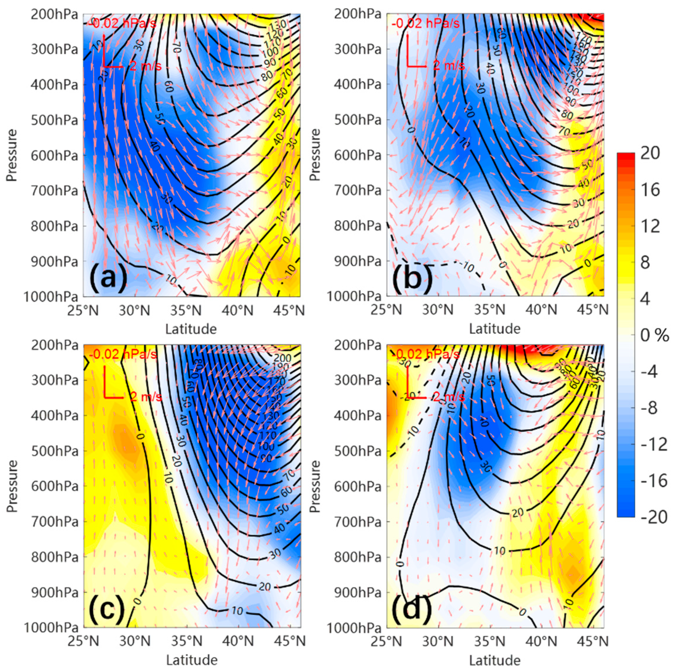
4. Warming Processes Associated with the Anticyclonic Circulation

To examine the vertical physical processes that are related to the four hot periods of the heatwave, we composed the vertical geopotential height anomalies, v-omega anomalies and relative humidity anomalies of region B from land surface to 200 hPa, which is shown in Figure 6. From Figure 6a–d, geopotential height anomalies, negative relative humidity anomalies and anomalous sinking flow have similar meridional movements as the hot regions in Figure 3 and the heatwave anticyclones in Figure 4.
In period 1, the dry condition appears to spread from the land surface to the upper troposphere with a northward inclination (Figure 6a). A strong downdraft can be seen in the subtropical latitudes. From south to north, the downward wind weakens and the southern flow intensifies. Because the extreme hot temperatures are mainly situated south of 40° N, both dry air adiabatic subsidence and southerly warm advection seems to be important for this period. Compared with period 1, the dry zone occurs at higher levels and moves further north in period 2 (Figure 6b). In addition, the positive geopotential height anomalies intensify and have a northward displacement. The downdraft transitions are close to 35° N, with a northerly component to the north and a southerly component to the south. Thus, the hot extremes south of 35° N can be explained by adiabatic warming, while north of 35° N, adiabatic warming and a southerly wind influence the development of extreme temperatures. Figure 6c shows the third hot period, where extreme temperatures are presented in northeast China. Corresponding to the extreme temperatures, the main body of the anticyclonic centre, the dry region and the downdrift move to north of 35° N, while the latter shows a more organized configuration. Thus, the hot area of this period is partly influenced by the dry and strong downdraft. In contrast to the first two periods, moisture and upward flow occupy the subtropical latitudes. The variables during the last period show a different distribution, with a southward displacement of the anticyclone and weaker negative relative humidity anomalies (Figure 6d). Additionally, the vertical winds show descending in the higher latitudes and weak sinking in the lower latitudes. These transformations can explain the temperature distribution in which weak warming occurs at lower latitudes and cooling occurs at higher latitudes during period 4.
Apart from the vertical physical processes, land surface heat fluxes are also essential to land surface temperature variations. The latitudinal distribution of surface heat flux (SSR, STR, SSHF and SLHF) anomalies and cloud cover (TCC, HCC, MCC and LCC) anomalies in region B are shown in Figure 7, which can also explain the evolution of the hot patterns for all four periods. The SSR anomalies are positive in the lower latitudes during period 1 and the anomalies gradually move to the higher latitudes, passing through period 2 and period 3. Finally, the enhanced SSR moves back to the lower latitudes in period 4. However, the STR, SSHF and SLHF anomalies generally have opposing changes to SSR anomalies, which indicates that the SSR is the main surface flux for land surface warming. After absorbing solar radiation, the land surface releases energy and warms the atmosphere in the form of STR, SSHF and SLHF. The SLHF is a predominant warming source in mideastern China as a result of the humid land surface. Additionally, Figure 7 implies also that the enhanced SSR is related to reduced cloud cover in different levels in the troposphere. HCC reduction is the largest among three cloud cover levels during period 2 and period 3, which can be attributed to the especially strong anticyclone and sinking movement, while the reduced cloud cover among different levels does not show clear differences during period 1 and period 4.
We conclude that the heatwave anticyclone in the troposphere is essential for heatwave formation. The increase in surface temperatures is related to adiabatic warming due to subsidence (corresponding to the anticyclone), clear sky conditions (increasing insolation) and the advection of warm air masses from the south. However, the roles of adiabatic compression and warm advection are latitude-dependent during the different hot periods.

5. The Role of Large-Circulation Patterns for the 2018 Heatwave
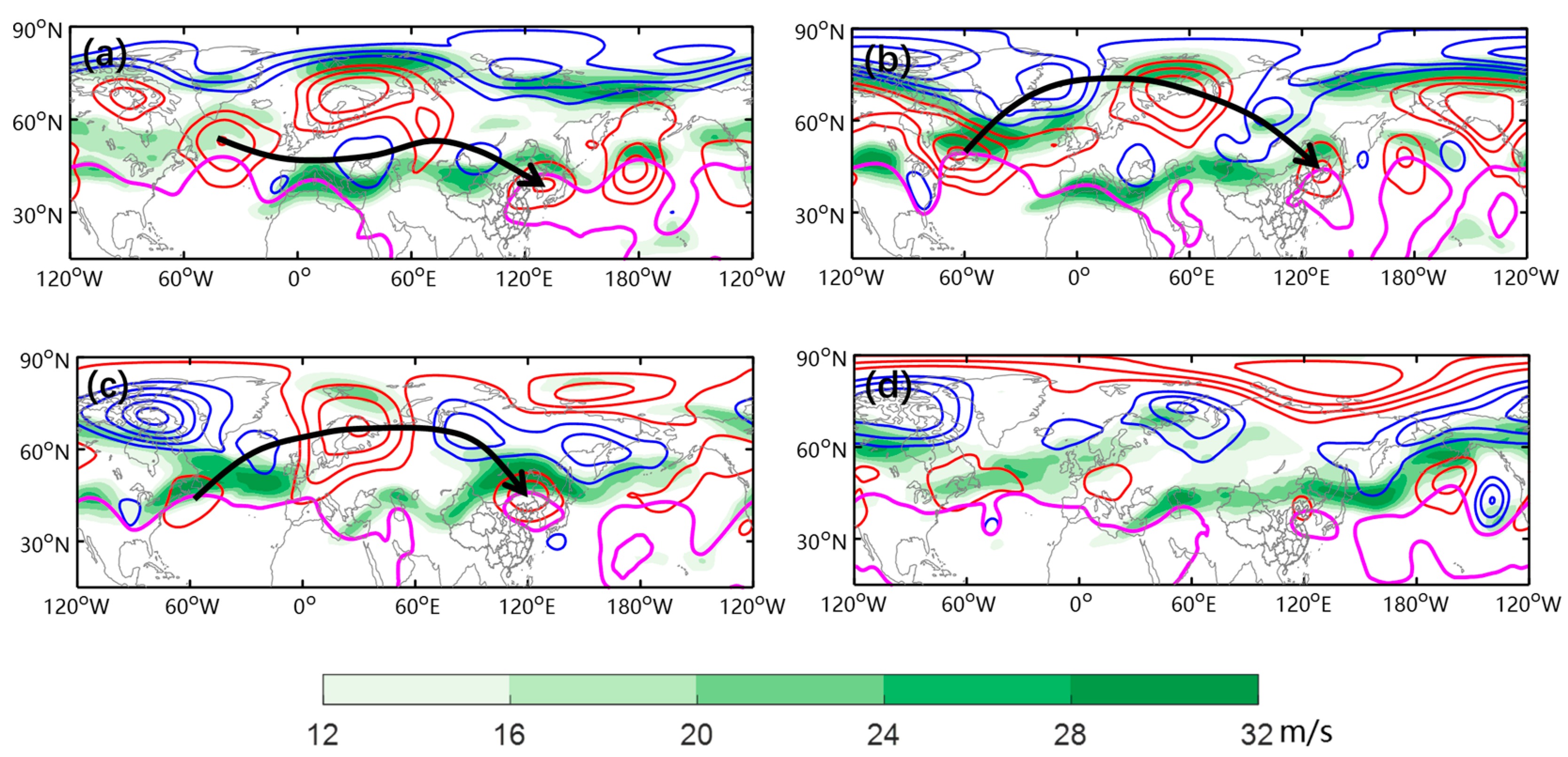
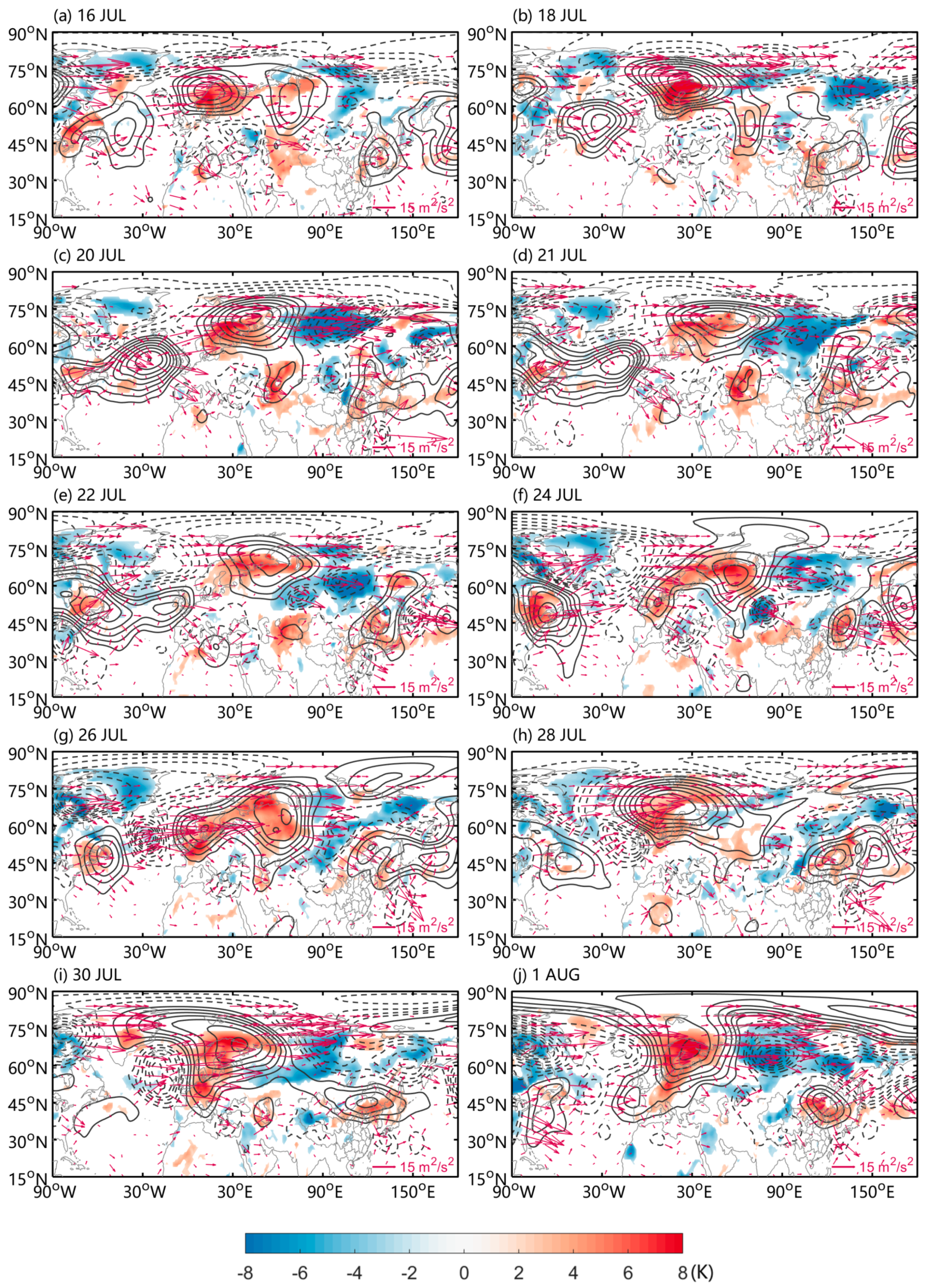
Since the heatwave of summer 2018 was excessively long as it sustained for 33 days, this heatwave should be treated as an intraseasonal event instead of a weather event, which is associated with different circulation patterns: high latitude wave train, midlatitude wave train and the WPSH, as discussed in Section 3. To better explain the long duration of the heatwave, we further examined the different circulation patterns and their formation processes.

5.1. Wave Trains

The high latitude wave train originating from the NAO+ over the North Atlantic contains a blocking high over the Scandinavia-Ural region with a duration of 18 days, which can be seen as a long-lived blocking event according to Luo et al. [51]. Many studies have shown that the persistence of a blocking high is favourable to extreme events such as cold waves, heatwaves and floods in the Northern Hemisphere [26,40,52]. To determine the exact role of the blocking high in the long-lived heatwave, the time-longitude evolution of the composite 500 hPa geopotential height anomalies averaged for 60°–75° N is given in Figure 8a. The blocking high has an eastward movement before 26 July and then shows a westward movement. During the blocked episode, three maxima can be identified around 18 July, 26 July and 1 August. The sustainability of the blocking is favourable for maintaining a stable mid-high latitude circulation pattern, which may contribute to extreme weather events. Moreover, during this heatwave, a quasi-stationary wave train with wavenumber-3 is clearly visible in the midlatitudes (60° W–150° E) between 16 and 21 July, which can also be traced back to the upstream NAO+ pattern, whose southern centre acts as a wave train source (Figure 8b). Although the wave train is recognized as set on 16 July, previous wave signals can be seen from the time-longitude geopotential height evolution, being also associated with the earlier existence of a strong positive NAO signal over the Atlantic (Figure 8b). In addition, the downstream positive and negative centre variations can be also seen clearly during the wave train period. However, the wave train with wavenumber-3 is transformed to a wave train with wavenumber-4 beginning on 22 July, which represents the end of the wavenumber-3 wave train.
To further examine the two wave trains and their energy transmissions, daily Eliassen-Palm fluxes are shown from 16 July to 1 August according to Plumb [53] (Figure 9a–j). In Figure 9, it is obvious that wave fluxes propagate to mideastern China mainly through the midlatitude wave train from 16 to 20 July, while the high latitude wave train moves to a downstream cyclone over the Central Siberian Plateau (about 100° E, 75° N) during this period (Figure 9a–c). However, starting from 22 July, the midlatitude wave train breaks down. Following the midlatitude wave train’s breakdown, wave fluxes continue to propagate to northeast China through the high latitude wave train (Figure 9e), which is sustained until 28 July (Figure 9e–h). Thus, the effect of the two wave trains can be compared to a relay process that is favourable to the persistence of the heatwave anticyclone over China. Notably, the heatwave anticyclone linked to the midlatitude wave train is situated over lower latitudes (Figure 9a–d) than the heatwave anticyclone related to the high latitude wave train (Figure 9e–h). In this case wave trains that are confined to different latitudes may affect the latitudinal position of the downstream circulations. We can conclude that the high latitude wave train and the midlatitude wave train together cause the heatwave anticyclone persistence, while the upstream blocking plays an essential role in stabilizing the mid-high latitude circulations.
Next, the role of jet streams is explored to explain the propagation of the two wave trains. The 300 hPa zonal wind anomalies and the 500 hPa geopotential height anomalies are composed during 16–21 July and 22–28 July, respectively (Figure 10).
In Figure 10a, the midlatitude wave train and the two segregated jets can be seen clearly. The northern jet surrounds the Arctic with a maximum north of the blocking, while the southern jet is situated at similar latitudes as the midlatitude wave train. Since the wave train propagation largely depends on the basic wind distribution [54], the jet stream can determine the wave train propagation direction as a wave guide. Then, we can infer that the intensified zonal wind at the midlatitudes is favourable for the midlatitude wave train to propagate to China, while the high latitude wave train mainly propagates along the high latitudes as a result of the intensified high latitude zonal wind. In contrast to Figure 10a, the zonal wind anomalies have three maxima over different latitudes, namely the north-western Atlantic, the Barents-Kara region and the east of the Baikal, while the midlatitude jet weakens with weak positive anomalies remaining over the Mediterranean (Figure 10b). Additionally, the zonal wind over the North Atlantic has a south-westward displacement and the NAO+ shows a northeast-southwest inclination, which avails the energy transport to the downstream areas to maintain the blocking high. Together with the intensified zonal wind over the area east of the Baikal, the high latitude wave train propagates to the midlatitudes.
From the discussion above, we know that persistent blocking and the midlatitude quasi-stationary wave train are the two essential factors for the heatwave. Both of them are related to the upstream NAO+ pattern over the North Atlantic. Thus, the NAO+ is seen as an initial atmospheric circulation pattern for the long-term heatwave, which is also an important wave source for the two wave trains. The time evolutions of the NAO+, the blocking and the midlatitude wave train are shown in Figure 11a. According to Kushnir et al. [55], the extratropical atmosphere responds to the changes in underlying SST distribution. To verify the relationship between the NAO+ and the anomalous SST patterns, the SST anomaly distributions over the North Atlantic sector are given in Figure 11b–c during the midlatitude wave train period (16–21 July) and the high latitude wave train period (22–28 July).
In Figure 11a, the blue line shows the time series of the normalized daily NAO index, which has 3 peaks between 1 July and 10 August. The red line represents the normalized wave train intensity that is larger than 1 standard deviation and the days marked by the red circle denote the midlatitude wave train period selected according to the aforementioned definition. However, before the wave train forms, there is also strong wave train intensity detected, which can be explained by the strong NAO+. The south positive centre of the NAO+ corresponds to a large geopotential height anomaly, which increases the wave train intensity according to the wave train intensity definition in Section 2.3. The 6 days related to a midlatitude wave train have the strongest intensities and 5 out of the 6 days have normalized intensities larger than 2 standard deviations, indicating that the wave train intensity defined in Section 2.3 is suitable. Moreover, the normalized blocking intensity (green line) and days of the blocking event (marked by green circles) are also shown in Figure 11a. The blocking intensity variation has two peaks during the event period with a minimum on 22–23 July. In particular, the first peak of the NAO variation is associated with the development of the midlatitude wave train 7 days later and with a first peak in the blocking intensity 10 days later. Seven days after the second peak of the NAO evolution, a second peak of the blocking intensity is visible. Thus, the NAO+ is assumed to be a precursor for the formation of the downstream blocking and the midlatitude wave train. To confirm the relationship between the NAO and the downstream blocking, their lead-lag correlations are also calculated. It is found that the largest correlation is equal to 0.77 (significant at the 0.01 level) and it appears when the NAO time series is prior to the blocking intensity by 5 days. It has been proposed in previous studies that the NAO+ may lead to downstream blocking formations in boreal winter [56,57]. Yao and Luo [56] found that the Ural Blocking generally lags the NAO dipole by 4–7 days in boreal winter, while the relationship between the NAO and the downstream blocking in boreal summer needs further study.
From Figure 11b–c, we find that the NAO+ is related to the north-south dipole pattern in the North Atlantic SST. When the midlatitude wave train plays a leading role in the heatwave (16–21 July), the south centre of the SST dipole mode has a wide longitudinal expansion. When the high latitude wave train takes effect, the south centre of the SST dipole shifts westwards and the corresponding NAO+ shows a northeast-southwest structure. The SST difference between the high and midlatitude wave train periods shows the positive SST anomaly intensification over the western Atlantic, which also indicates the westward movement of the south positive centre of the SST dipole (Figure 11d). Thus, the configuration is consistent with a link between the NAO+ and the SST dipole mode [58]. Also, the change in the NAO+ pattern and the corresponding zonal wind suggest the transition from a midlatitude wave train to a high latitude wave train. Further exploration shows also that the three months of the 2018 summer have high normalized NAO indices of 1.18, 1.46 and 2.01 for June, July and August, respectively, related to an SST dipole pattern in the North Atlantic sector for the summer. However, the reasons behind the formation of the NAO+ and the SST dipole and the causal relationships between the SST and circulation patterns over the North Atlantic sector are not determined, which require further study.

5.2. Western Pacific Subtropical High (WPSH)

Another important large-scale circulation pattern for the long-lived heatwave is the anomalous WPSH. Figure 12a shows the normalized indices for the WPSH area, intensity, west ridge point, north border and ridge line variations. During the earlier stage of the heatwave, the WPSH has a large area and high intensity. In addition, both the north border and ridge line indices are large, showing an increasing tendency. However, in the later period, the WPSH area and intensity decline sharply and remain low, while the north border and ridge line indices reach higher values with normalized intensities larger than 2 standard deviations. Thus, we can conclude that the more northward position of the WPSH is an important factor that acts throughout the entire heatwave. In addition, the normalized north border (ridge line) index with values larger than 1 standard deviation is sustained for 34 (49) days, which is also an essential contributor to the heatwave persistence. These results can also be verified in the time-latitude profile of the 500 hPa geopotential height anomalies and the 5880 gpm isoline at 500 hPa, which provides a more direct evidence about the movement and intensity variations of the WPSH (Figure 12b). However, the WPSH does not show an anomalous westward position during the heatwave. In a previous study, the northward movement of the WPSH was related to the variation in the stationary Rossby wave train along with the Asian jet [59]. Tao and Wei [59] found that the northward jump of the WPSH is linked to the Eurasian Rossby wave train. The stationary wave train favours wave energy propagating along the subtropical jet stream to eastern China, which influences the movement of the WPSH ridge. In our case, the heatwave is accompanied by the midlatitude wave train confined in the subtropical jet; thus, the northward movement of the WPSH may be explained by the findings of Tao and Wei [59]. However, more investigations are needed to reveal the physical mechanisms that lead to the persistent anomalous northward WPSH.

6. Discussion and Conclusions

This study provides a better understanding of the large-scale circulation patterns associated with the long-lived heatwave in mideastern China in summer 2018. This heatwave is the hottest event with the highest 33-days mean daily maximum temperature since 1979. Four hot periods are extracted from the heatwave to determine the spatiotemporal evolutions and associated circulation patterns of the heatwave. All four hot periods are associated with a heatwave anticyclone, which is the typical circulation pattern for heatwaves in mideastern China [9,35,60]. From period 1 to period 4, the high temperatures first move northward from the Yangtze River and the Yellow River to northeast China and then move back in accordance with the movement of the heatwave anticyclone, which is influenced by the variation of the WPSH and mid-high latitude wave trains.
Because the four hot periods are all related to a heatwave anticyclone over the hot region, the warming processes associated with the anticyclonic pattern are also examined. Considering the vertical structure of the heatwave anticyclone, both the sinking motion and the south wind are important factors to the heatwave, varying with latitude. Additionally, the warming process of the heatwave anticyclone enhances insolation by reducing cloud cover, which is generally consistent for the 4 hot periods.
Regarding the atmospheric circulation patterns, the relay of a midlatitude wave train and a high latitude wave train and the persistent north-displaced WPSH play important roles in the excessively long-lived heatwave. Both the midlatitude wave train and high latitude wave train originate from the NAO+ circulation over the North Atlantic sector. During the midlatitude wave train period, the Asian jet strengthens and acts as a wave guide for wave fluxes propagating from the south centre of the NAO+ to mideastern China. The high latitude wave train corresponds to three large positive zonal wind anomaly centres situated over the north-western Atlantic, Barents-Kara region and east of Baikal, which avails the high latitude wave train to propagate to northeast China. The transition from the midlatitude wave train to a high latitude wave train can explain the northward shift of the heatwave anticyclone. In addition, the upstream blocking is also persistent, with a duration of 18 days, which plays a role in stabilizing the mid-high latitude wave trains. During the propagation of the two wave trains, NAO+ acts as a wave flux origin. The first peak of the NAO is associated with the maximum of the wave train intensity and the first maximal value of the blocking intensity, while the second peak of the NAO is associated with the second maximum of the blocking intensity, implying the downstream wave energy propagation originating from the NAO+ circulation pattern [61]. In addition, a dipole SST pattern in the northern Atlantic is present in summer 2018, which may contribute to the NAO pattern. The anomalous WPSH can also explain the long-lived heatwave because the WPSH has a prolonged northward displacement with normalized north border (ridge line) indices larger than 1 standard deviation for 34 (49) days. Additionally, the area and intensity indices of the WPSH are large during the earlier stage of the heatwave. Particularly, the high latitude wave train and the northward WPSH explain why it was extremely hot in northeast China, with the maximum temperatures of many weather stations breaking historical records.
Notably, northern Europe also suffered from extremely hot weather, while the temperature exceeded 30 °C inside the Arctic Circle during the summer of 2018, which attracted much attention. The extremely hot weather in Europe is implied to have a teleconnection relationship with the heatwave in China through the propagation of wave trains, specifically the high latitude wave train, which requires further study. In addition, there are also extremely high temperatures in Japan and the Korean Peninsula, both of which experienced the same heatwave anticyclone as mideastern China.
In this study, the heatwave in mideastern China is shown to have a link to the NAO+ over the North Atlantic, however, the mechanisms associated with the relationships between the NAO+ and SST dipole mode are not examined. Also the reasons behind the unusual northward displacement of the WPSH are not studied. These may be important factors for the summer heatwave prediction. In the future, the interactions between the atmospheric circulations and SST modes should be further investigated to reveal more potential predictors for summer heatwaves.

Author Contributions

Y.Y. conceived and carried out the project, and M.L. wrote the paper; D.L. and L.Z. constructively reviewed the paper.

Funding

This research was funded by the National Natural Science Foundation of China (Grant numbers: 41430533) and the National key research and development program of China (2016YFA0601802) and the APC was funded by the National Natural Science Foundation of China (Grant numbers: 41430533).

Acknowledgments

The authors thank two anonymous reviewers for valuable comments that improved this paper.

Conflicts of Interest

The authors declare no conflict of interest.

References

  1. Meehl, G.A.; Tebaldi, C. More intense, more frequent and longer lasting heat waves in the 21st century. Science 2004, 305, 994–997. [Google Scholar] [CrossRef] [PubMed]
  2. Perkins, S.E.; Alexander, L.V.; Nairn, J.R. Increasing frequency, intensity and duration of observed global heatwaves and warm spells. Geophys. Res. Lett. 2012, 39, 20714. [Google Scholar] [CrossRef]
  3. Ding, T.; Qian, W.H.; Yan, Z.W. Changes in hot days and heat waves in China during 1961–2007. Int. J. Climatol. 2010, 30, 1452–1462. [Google Scholar] [CrossRef]
  4. Ding, T.; Ke, Z.J. Characteristics and changes of regional wet and dry heat wave events in China during 1960–2013. Theor. Appl. Climatol. 2015, 122, 651–665. [Google Scholar] [CrossRef]
  5. Zhang, J.; Liu, Z.Y.; Chen, L. Reduced soil moisture contributes to more intense and more frequent heat waves in northern China. Adv. Atmos. Sci. 2015, 32, 1197–1207. [Google Scholar] [CrossRef]
  6. Chen, Y.; Li, Y. An inter–comparison of three heat wave types in China during 1961–2010: Observed basic features and linear trends. Sci. Rep. 2017, 7, 45619. [Google Scholar] [CrossRef]
  7. Li, Y.; Ding, Y.H.; Li, W.J. Observed trends in various aspects of compound heat waves across China from 1961 to 2015. J. Meteorol. Res. 2017, 31, 455–467. [Google Scholar] [CrossRef]
  8. Luo, M.; Lau, N.C. Heat waves in Southern China: Synoptic behavior, long–term change and urbanization effects. J. Clim. 2017, 30, 703–720. [Google Scholar] [CrossRef]
  9. Freychet, N.; Tett, S.; Wang, J.; Hegerl, G. Summer heat waves over Eastern China: Dynamical processes and trend attribution. Environ. Res. Lett. 2017, 12, 2. [Google Scholar] [CrossRef]
  10. Sun, Y.; Zhang, X.B.; Zwiers, F.W.; Song, L.C.; Wan, H.; Hu, T.; Yin, H.; Ren, G.Y. Rapid increase in the risk of extreme summer heat in Eastern China. Nat. Clim. Chang. 2014, 4, 1082–1085. [Google Scholar] [CrossRef]
  11. Yang, J.; Yin, P.; Sun, J.M.; Wang, B.G.; Zhou, M.G.; Li, M.M.; Tong, S.L.; Meng, B.H.; Guo, Y.M.; Liu, Q.Y. Heatwave and mortality in 31 major Chinese cities: Definition, vulnerability and implications. Sci. Total Environ. 2019, 649, 695–702. [Google Scholar] [CrossRef]
  12. Campbell, S.; Remenyi, T.A.; White, C.J.; Johnston, F.H. Heatwave and health impact research: A global review. Health Place 2018, 53, 210–218. [Google Scholar] [CrossRef]
  13. Flach, M.; Sippel, S.; Gans, F.; Bastos, A.; Brenning, A.; Reichstein, M.; Mahecha, M.D. Contrasting biosphere responses to hydrometeorological extremes: Revisiting the 2010 western Russian heatwave. Biogeosciences 2018, 15, 6067–6085. [Google Scholar] [CrossRef]
  14. Telesca, V.; Lay–Ekuakille, A.; Ragosta, M.; Giorgio, G.A.; Lumpungu, B. Effects on public health of heat waves to improve the urban quality of life. Sustainability 2018, 10, 1082. [Google Scholar] [CrossRef]
  15. Black, E.; Blackburn, M.; Harrison, G.; Hoskins, B.; Methven, J. Factors contributing to the summer 2003 European heatwave. Weather 2010, 59, 217–223. [Google Scholar] [CrossRef]
  16. Barriopedro, D.; Fischer, E.M.; Luterbacher, J.; Trigo, R.M.; García–Herrera, R. The hot summer of 2010: Redrawing the temperature record map of Europe. Science 2011, 332, 220–224. [Google Scholar] [CrossRef] [PubMed]
  17. Katsafados, P.; Papadopoulos, A.; Varlas, G.; Papadopoulou, E.; Mavromatidis, E. Seasonal predictability of the 2010 Russian heat wave. Nat. Hazard Earth Sys. 2014, 14, 1531–1542. [Google Scholar] [CrossRef] [Green Version]
  18. Quandt, L.A.; Keller, J.H.; Martius, O.; Jones, S.C. Forecast variability of the blocking system over Russia in summer 2010 and its impact on surface conditions. Weather Forecast. 2017, 32, 61–82. [Google Scholar] [CrossRef]
  19. Duan, H.X.; Wang, S.P.; Feng, J.Y. The national drought situation and its impacts and causes in the summer 2013. J. Arid Meteorol. 2013, 31, 633–640. [Google Scholar]
  20. Sparrow, S.; Su, Q.; Tian, F.X.; Li, S.H.; Chen, Y.; Chen, W.; Luo, F.F.; Freychet, N.; Lott, F.C.; Dong, B.W.; et al. Attributing human influence on the July 2017 Chinese heatwave: The influence of sea–surface temperatures. Environ. Res. Lett. 2018, 13, 11. [Google Scholar] [CrossRef]
  21. Wang, G.F.; Ye, D.X.; Zhang, Y.X.; Huang, D.P.; Hou, W. Characteristics and abnormal atmospheric circulation of regional high temperature process in 2017 over China. Prog. Inquisitiones DE Mutat. Clim. 2018, 14, 341–349. (In Chinese) [Google Scholar]
  22. Stefanon, M.; D’Andrea, F.; Drobinski, P. Heatwave classification over Europe and the Mediterranean region. Environ. Res. Lett. 2012, 7, 1. [Google Scholar] [CrossRef]
  23. Perkins, S.E.; Argueso, D.; White, C.J. Relationships between climate variability, soil moisture and Australian heatwaves. J. Geophys. Res. Atmos. 2015, 120, 8144–8164. [Google Scholar] [CrossRef]
  24. Rex, D.F. Blocking action in the middle troposphere and its effect upon regional climate: I. An aerological study of blocking action. Tellus 1950, 2, 196–211. [Google Scholar] [CrossRef]
  25. Rex, D.F. Blocking action in the middle troposphere and its effect upon regional climate: II. The climatology of blocking action. Tellus 1950, 2, 275–301. [Google Scholar]
  26. Wagner, A.J. Weather and circulation of January 1969—Continued strong high-latitude blocking and flood-producing rains in California. Mon. Weather Rev. 1969, 97, 351–358. [Google Scholar] [CrossRef]
  27. Lyon, B.; Dole, R.M. A diagnostic comparison of the 1980 and 1988 US summer heat wave-droughts. J. Clim. 1995, 8, 1658–1675. [Google Scholar] [CrossRef]
  28. Athar, H.; Lupo, A.R. Scale analysis of blocking events from 2002 to 2004: A case study of an unusually persistent blocking event leading to a heat wave in the Gulf of Alaska during August 2004. Adv. Meteorol. 2010, 2010, 1–15. [Google Scholar] [CrossRef]
  29. Schaller, N.; Sillmann, J.; Anstey, J.; Fischer, E.M.; Grams, C.M.; Russo, S. Influence of blocking on Northern European and Western Russian heatwaves in large climate model ensembles. Environ. Res. Lett. 2018, 13, 5. [Google Scholar] [CrossRef]
  30. Hauser, M.; Orth, R.; Seneviratne, S.I. Role of soil moisture versus recent climate change for the 2010 heat wave in Western Russia. Geophys. Res. Lett. 2016, 43, 2819–2826. [Google Scholar] [CrossRef]
  31. Petoukhov, V.; Rahmstorf, S.; Petri, S.; Schellnhuber, H.J. Quasiresonant amplification of planetary waves and recent Northern Hemisphere weather extremes. Proc. Natl. Acad. Sci. USA 2013, 110, 5336–5341. [Google Scholar] [CrossRef] [Green Version]
  32. Ding, Q.H.; Wang, B. Circumglobal teleconnection in the Northern Hemisphere summer. J. Clim. 2005, 18, 3483–3505. [Google Scholar] [CrossRef]
  33. Hong, X.W.; Lu, R.Y.; Li, S.L. Amplified summer warming in Europe–West Asia and Northeast Asia after the mid-1990s. Environ. Res. Lett. 2017, 12, 9. [Google Scholar] [CrossRef]
  34. Sanchez–Benitez, A.; Garcia–Herrera, R.; Barriopedro, D.; Sousa, P.M.; Trigo, R.M. June 2017: The earliest European summer mega–heatwave of reanalysis period. Geophys. Res. Lett. 2018, 45, 1955–1962. [Google Scholar] [CrossRef]
  35. Li, J.; Ding, T.; Jia, X.L.; Zhao, X.C. Analysis on the extreme heat wave over China around Yangtze River region in the Summer of 2013 and its main contributing factors. Adv. Meteorol. 2015, 2015, 1–15. [Google Scholar] [CrossRef]
  36. Kim, K.Y.; Roh, J.W.; Lee, D.K.; Jhun, J.G. Physical mechanisms of the seasonal, subseasonal and high-frequency variability in the seasonal cycle of summer precipitation in Korea. J. Geophys. Res. Atmos. 2010, 115, D14110. [Google Scholar] [CrossRef]
  37. Dee, D.P.; Uppala, S.M.; Simmons, A.J.; Berrisford, P.; Poli, P.; Kobayashi, S.; Andrae, U.; Balmaseda, M.A.; Balsamo, G.; Bauer, P.; et al. The ERA–Interim reanalysis: Configuration and performance of the data assimilation system. Q. J. Roy. Meteor. Soc. 2011, 137, 553–597. [Google Scholar] [CrossRef]
  38. Barnston, A.G.; Livezey, R.E. Classification, seasonality and persistence of low-frequency atmospheric circulation patterns. Mon. Wea. Rev. 1987, 115, 1083–1126. [Google Scholar] [CrossRef]
  39. Huang, J.B.; Zhang, X.D.; Zhang, Q.Y.; Lin, Y.L.; Hao, M.J.; Luo, Y.; Zhao, Z.C.; Yao, Y.; Chen, X.; Wang, L.; et al. Recently amplified arctic warming has contributed to a continual global warming trend. Nat. Clim. Chang. 2017, 7, 875–879. [Google Scholar] [CrossRef]
  40. Yao, Y.; Luo, D.H.; Dai, A.G.; Simmonds, I. Increased quasi stationarity and persistence of winter Ural blocking and Eurasian extreme cold events in response to Arctic warming. Part I: Insights from Observational Analyses. J. Clim. 2017, 30, 3549–3568. [Google Scholar] [CrossRef]
  41. Tibaldi, S.; Molteni, F. On the operational predictability of blocking. Tellus 1990, 42, 343–365. [Google Scholar] [CrossRef]
  42. Screen, J.A.; Simmonds, I. Amplified mid-latitude planetary waves favour particular regional weather extremes. Nat. Clim. Chang. 2014, 4, 704–709. [Google Scholar] [CrossRef] [Green Version]
  43. Coumou, D.; Petoukhov, V.; Rahmstorf, S.; Petri, S.; Schellnhuber, H.J. Quasi-resonant circulation regimes and hemispheric synchronization of extreme weather in boreal summer. Proc. Natl. Acad. Sci. USA 2014, 111, 12331–12336. [Google Scholar] [CrossRef] [Green Version]
  44. Li, J.N.; Meng, W.G.; Wang, A.Y.; Liu, L.M.; Feng, R.Q.; Hou, E.B. Climatic characteristics of the intensity and position of the subtropical high in the western Pacific. Trop. Geogr. 2003, 23, 35–39. (In Chinese) [Google Scholar]
  45. Liu, Y.Y.; Li, W.J.; Ai, M.X.; Li, Q.Q. Reconstruction and application of the monthly western Pacific subtropical high indices. J. Appl. Meteorol. Sci. 2012, 23, 414–423. (In Chinese) [Google Scholar]
  46. Wang, F.; Zhang, J.Y.; Gu, X.P.; Du, X.L.; Wu, G.H. Relationshio between the western Pacific subtropical high’s characteristic index and summer precipitation over Guizhou. Torrential Rain Disasters 2017, 36, 348–356. (In Chinese) [Google Scholar]
  47. Perkins, S.E.; Alexander, L.V. On the measurement of heat waves. J. Clim. 2013, 26, 4500–4517. [Google Scholar] [CrossRef]
  48. Grotjahn, R.; Black, R.; Leung, R.; Wehner, M.F.; Barlow, M.; Bosilovich, M.; Gershunov, A.; Gutowski, W.J.; Gyakum, J.R.; Katz, R.W.; et al. Prabhat, North American extreme temperature events and related large scale meteorological patterns: a review of statistical methods, dynamics, modeling and trends. Clim. Dyn. 2016, 46, 1151–1184. [Google Scholar] [CrossRef]
  49. Horton, R.M.; Lesk, C.; Mankin, J.S. A review of recent advances in research on extreme heat events. Curr. Clim. Chang. Rep. 2016, 2, 242–259. [Google Scholar] [CrossRef]
  50. Thompson, D.W.J.; Wallace, J.M. The Arctic Oscillation signature in wintertime geopotential height and temperature fields. Geophys. Res. Lett. 1998, 25, 1297–1300. [Google Scholar] [CrossRef]
  51. Luo, D.H.; Lupo, A.R.; Wan, H. Dynamics of eddy-driven low-frequency dipole modes. Part I: A simple model of North Atlantic oscillations. J. Atmos. Sci. 2007, 31, 3–28. [Google Scholar] [CrossRef]
  52. Dong, L.; Mitra, C.; Greer, S.; Burt, E. The dynamical linkage of atmospheric blocking to drought, heatwave and urban heat island in Southeastern US: A multi–scale case study. Atmosphere 2018, 9, 33. [Google Scholar] [CrossRef]
  53. Plumb, R.A. On the three–dimensional propagation of stationary waves. J. Atmos. Sci. 1985, 42, 217–229. [Google Scholar] [CrossRef]
  54. Naoe, H.; Matsuda, Y.; Nakamura, H. Rossby wave propagation in idealized and realistic zonally varying flows. J. Meteorol. Soc. Jpn. 1997, 75, 687–700. [Google Scholar] [CrossRef]
  55. Kushnir, Y.; Robinson, W.A.; Blade, I.; Hall, N.M.J.; Peng, S.; Sutton, R. Atmospheric GCM response to extratropical SST anomalies: Synthesis and evaluation. J. Clim. 2002, 15, 2233–2256. [Google Scholar] [CrossRef]
  56. Yao, Y.; Luo, D.H. Do European blocking events precede North Atlantic Oscillation events? Adv. Atmos. Sci. 2015, 32, 1106–1118. [Google Scholar] [CrossRef]
  57. Yao, Y.; Luo, D.H. An asymmetric space-time connection of Euro-Atlantic blocking within the NAO life cycle and European climates. Adv. Atmos. Sci. 2018, 35, 46–62. [Google Scholar] [CrossRef]
  58. Peng, S.L.; Robinson, W.A.; Li, S.L. Mechanisms for the NAO responses to the North Atlantic SST tripole. J. Clim. 2003, 16, 1987–2004. [Google Scholar] [CrossRef]
  59. Tao, S.Y.; Wei, J. Severe snow and freezing–rain in January 2008 in the Southern China. Clim. Environ. Res. 2008, 13, 337–350. (In Chinese) [Google Scholar]
  60. Wang, W.W.; Zhou, W.; Li, X.Z.; Wang, X.; Wang, D.X. Synoptic–scale characteristics and atmospheric controls of summer heat waves in China. Clim. Dyn. 2016, 46, 2923–2941. [Google Scholar] [CrossRef]
  61. Luo, D.H.; Zhou, W.; Wei, K. Dynamics of eddy–driven North Atlantic Oscillations in a localized shifting jet: zonal structure and downstream blocking. Clim. Dyn. 2010, 34, 73–100. [Google Scholar] [CrossRef]
Figure 1. Station distribution in China. Stations with consecutive missing data for more than 2 days are excluded and a total of 555 stations are selected. The green point denotes Shenyang, the provincial capital of the Liaoning Province and the blue point represents Changchun, the provincial capital of the Jilin Province.
Atmosphere 10 00089 g001
Figure 2. (a) Composite maximum surface air temperature (SAT) anomalies for 15 July–15 August. The extreme hot region (region A) for the heatwave is marked with black lines. The region in the parallelogram (region B) is used to study the evolution of the heatwave. Two hot spots in region A are denoted by green lines (region C) and blue lines (region D), respectively. (b) Time-latitude evolution of normalized SAT anomalies averaged over region B, where the thick black arrow denotes the movement of the hot region. Variations in the domain-averaged SAT anomalies (blue line with dots) for region C and region D are shown in (c,d). The red dashed lines indicate the 0.75 (−0.75) standard deviation and the four hot periods selected by the 0.75 standard deviation are marked by transparent green shadings.
Atmosphere 10 00089 g002
Figure 3. Composite SAT anomalies for (a) hot period 1 (14–20 July), (b) hot period 2 (20–25 July), (c) hot period 3 (27 July–4 August) and (d) hot period 4 (4-12 August).
Atmosphere 10 00089 g003aAtmosphere 10 00089 g003b
Figure 4. Composite 500 hPa geopotential height anomalies (contours; interval = 40; units: gpm), 300 hPa zonal wind (shading; units: m/s), 5880 gpm isoline (pink) for (a) hot period 1, (b) hot period 2, (c) hot period 3 and (d) hot period 4. The red (blue) contours address positive (negative) 500 hPa geopotential height anomalies. The thick black arrows denote the midlatitude wave train in (a) and the high latitude wave trains in (b,c).
Atmosphere 10 00089 g004
Figure 5. Composite 850-hPa horizontal wind anomalies (vectors; units: m/s) for (a) hot period 1, (b) hot period 2, (c) hot period 3 and (d) hot period 4. Only wind vectors larger than 2 m/s are shown.
Atmosphere 10 00089 g005
Figure 6. Zonally averaged geopotential height anomalies (contours; interval = 10; units: gpm), relative humidity anomalies (shading; units: %) and v-omega anomalies (vectors; units are labelled in the figure) over region B from the land surface to 200 hPa for (a) hot period 1, (b) hot period 2, (c) hot period 3 and (d) hot period 4.
Atmosphere 10 00089 g006
Figure 7. Zonally averaged surface solar radiation (SSR, yellow line), surface thermal radiation (STR, red line), surface sensible heat flux (SSHF, blue line) and surface latent heat flux (SLHF, green line) anomalies in region B for (a) hot period 1, (c) hot period 2, (e) hot period 3 and (g) hot period 4. Additionally, zonally averaged total cloud cover (TCC, black line), low cloud cover (LCC, blue line), medium cloud cover (MCC, green line) and high cloud cover (HCC, red line) anomalies in region B are shown in (b,d,f,h) for hot periods 1–4.
Atmosphere 10 00089 g007
Figure 8. Time-longitude evolution of the 500 hPa geopotential height anomalies averaged over the latitudes 60°–75° N and 40°–55° N, representing the evolution of (a) the blocking and (b) the wave train, respectively. The thick black arrow in (a) denotes the movement of the blocking.
Atmosphere 10 00089 g008
Figure 9. Daily 500 hPa geopotential height anomalies (contours, interval = 30; units: gpm), SAT anomalies (shading; units: K) and horizontal components of the wave fluxes (arrows; units: m2/s2) from 16 July to 1 August (aj represent the instantaneous daily evolutions). The solid (dashed) contours show positive (negative) 500 hPa geopotential height anomalies.
Atmosphere 10 00089 g009
Figure 10. Composite 500 hPa geopotential height anomalies (contours, interval = 30; units: gpm) and 300 hPa zonal wind anomalies (shading; units: m/s) for (a) the midlatitude wave train period (16–21 July) and (b) the high latitude wave train period (22–28 July). The solid (dashed) contours denote positive (negative) 500 hPa geopotential height anomalies.
Atmosphere 10 00089 g010
Figure 11. (a) Daily variations in the normalized NAO index (blue line), blocking intensity index (green line) and midlatitude wave train intensity index (red line). The red circles denote the days of the midlatitude wave train and the green circles represent the blocked days. The 1 (−1) standard deviation is denoted by the red dashed line. Sea surface temperature (SST) anomalies for the (b) midlatitude wave train period (16–21 July) (c) high latitude wave train period (22–28 July) and (d) the difference between (b) and (c) over the northern Atlantic sector.
Atmosphere 10 00089 g011
Figure 12. (a) Daily time series of normalized area (blue), intensity (green), west ridge point (red), north border (violet) and ridge line (orange) indices for WPSH. (b) Time-latitude evolution of the 500 hPa geopotential height anomalies averaged over the region from 115° to 140° E. The solid black line denotes the variation in the 5880 gpm isoline at 500 hPa.
Atmosphere 10 00089 g012

