
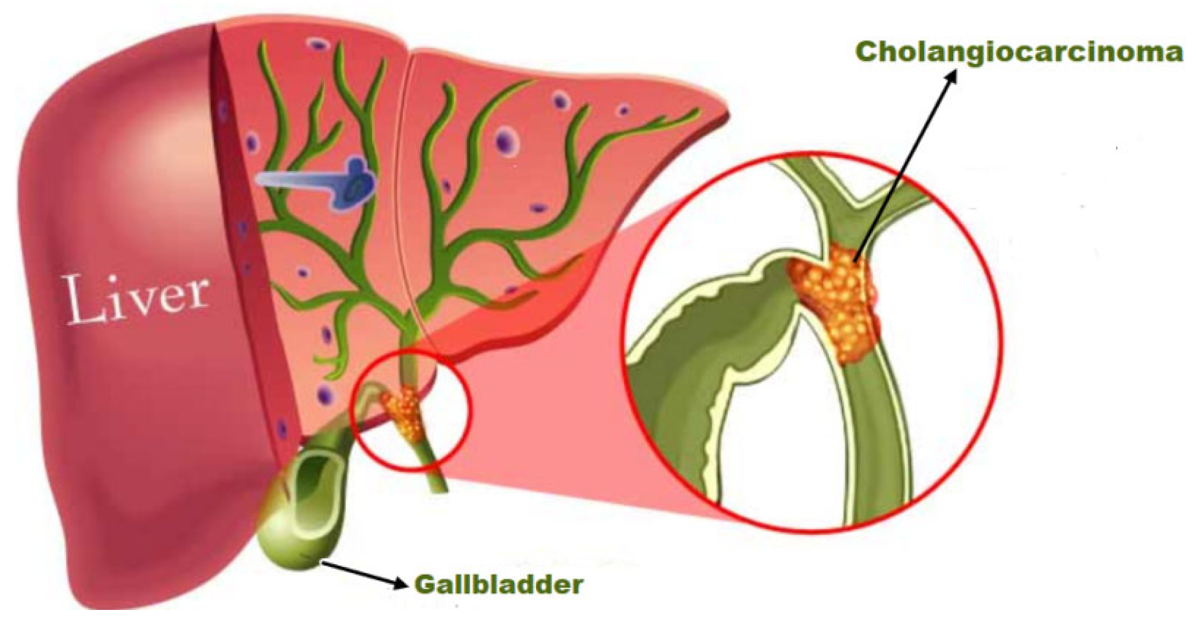
EDLM: Ensemble Deep Learning Model to Detect Mutation for the Early Detection of Cholangiocarcinoma
 , ,
, ,
Abstract
:1. Introduction
2. Materials and Methods
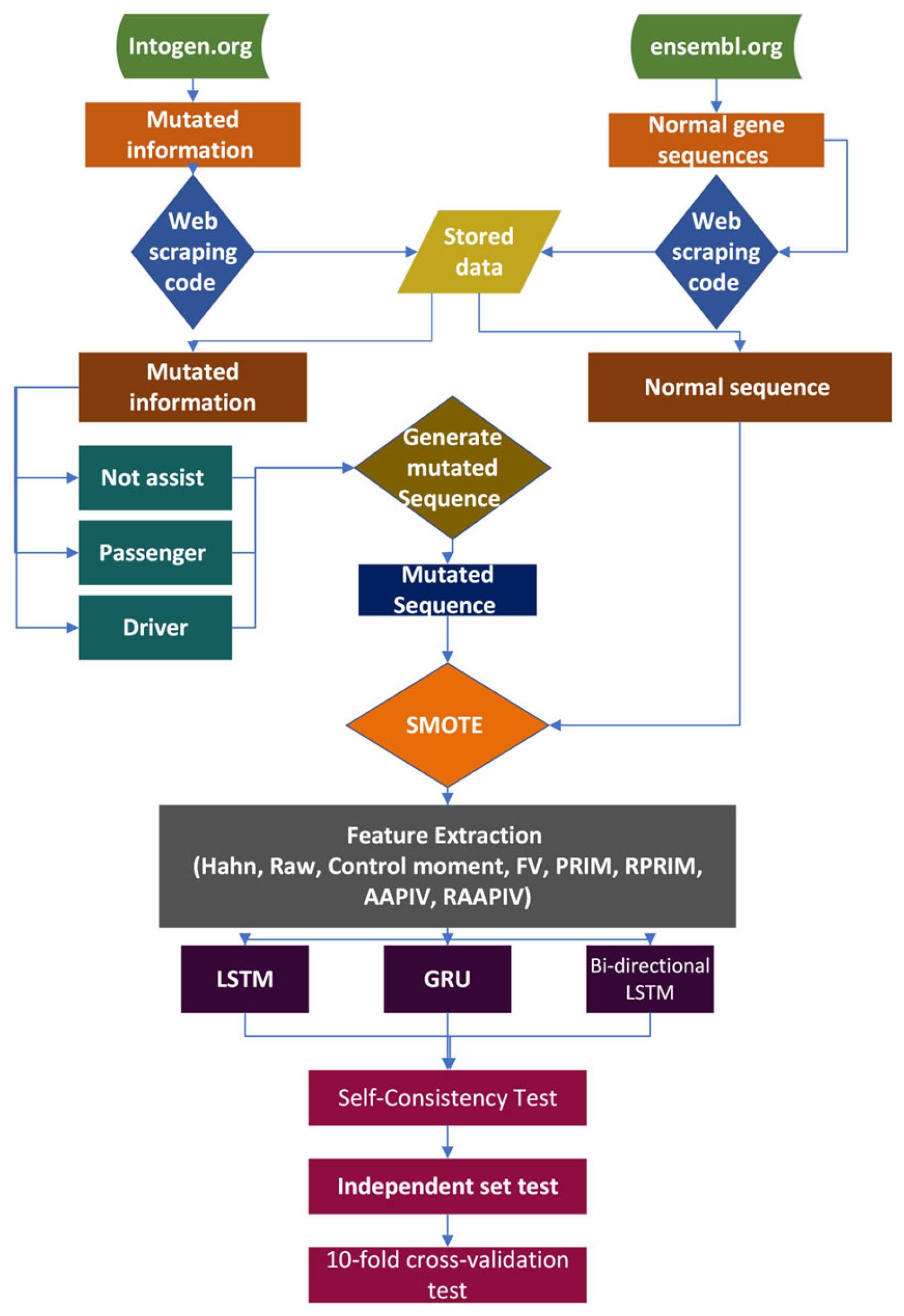
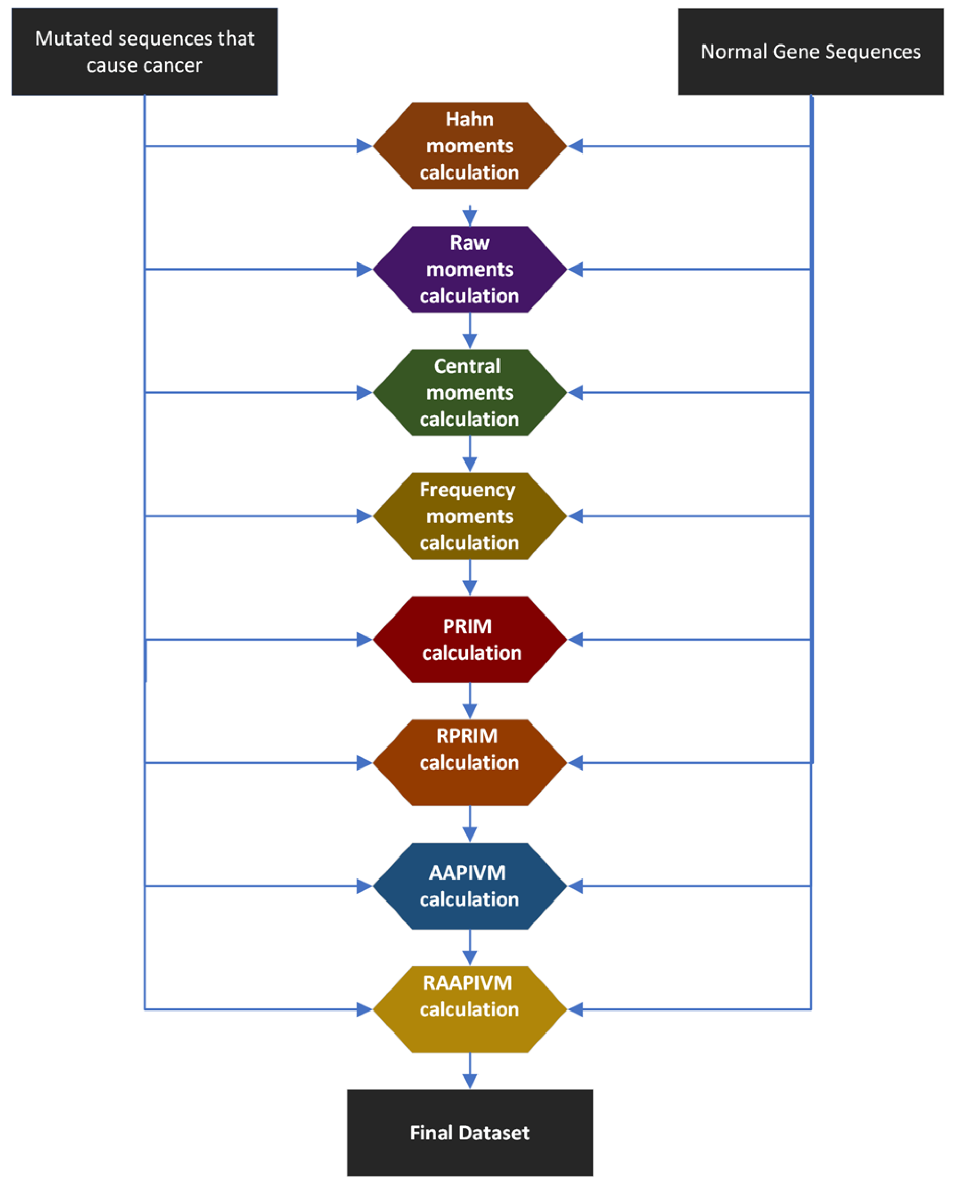
2.1. Data Acquisition Framework
2.2. Feature Extraction
2.2.1. Hahn Moments Calculation
2.2.2. Central Moments Calculation
2.2.3. Raw Moments Calculation
2.2.4. Position Relative Incidence Matrix (PRIM)
2.2.5. Reverse Position Relative Incidence Matrix (RPRIM)
2.2.6. Accumulative Absolute Position Incidence Vector (AAPIV)
2.2.7. Reverse Accumulative Absolute Position Incidence Vector (RAAPIV)
2.2.8. Frequency Vector Calculation
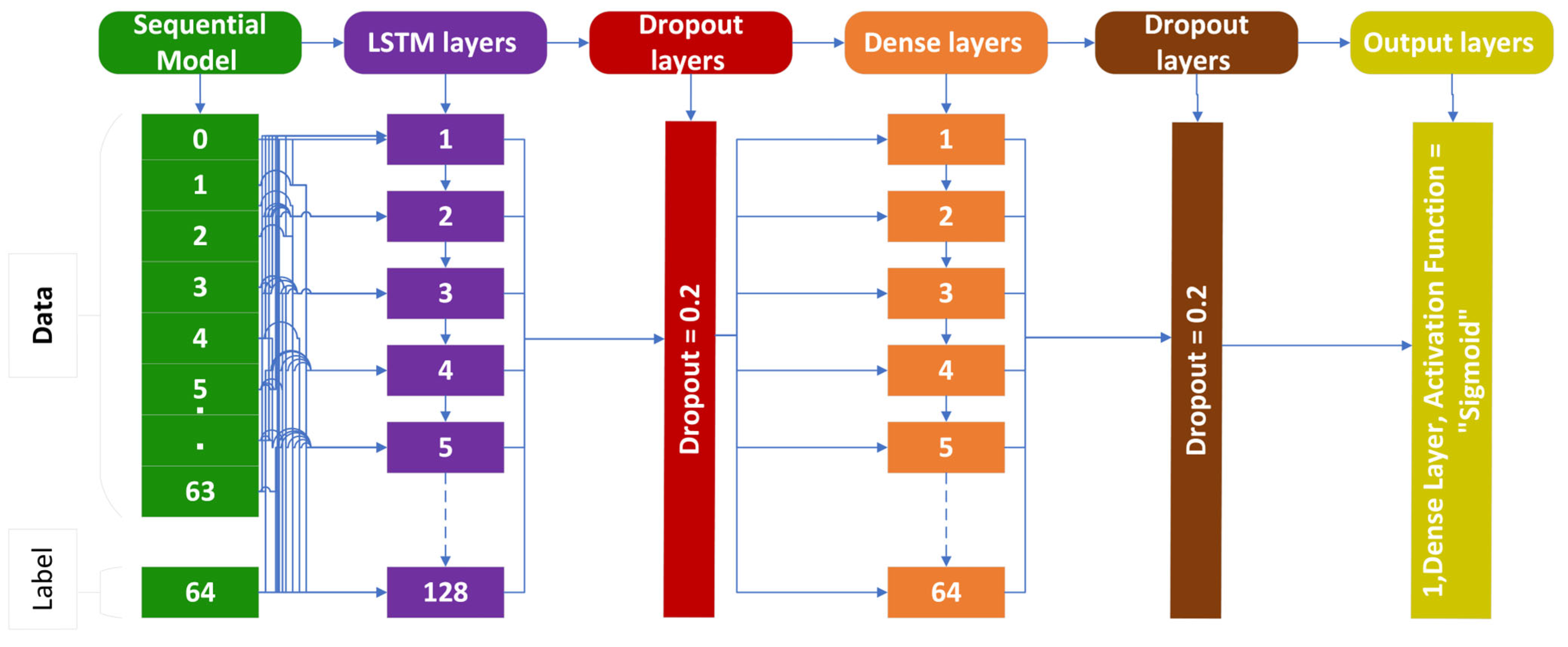
3. Proposed Deep Learning Algorithms
3.1. Long Short-Term Memory (LSTM)
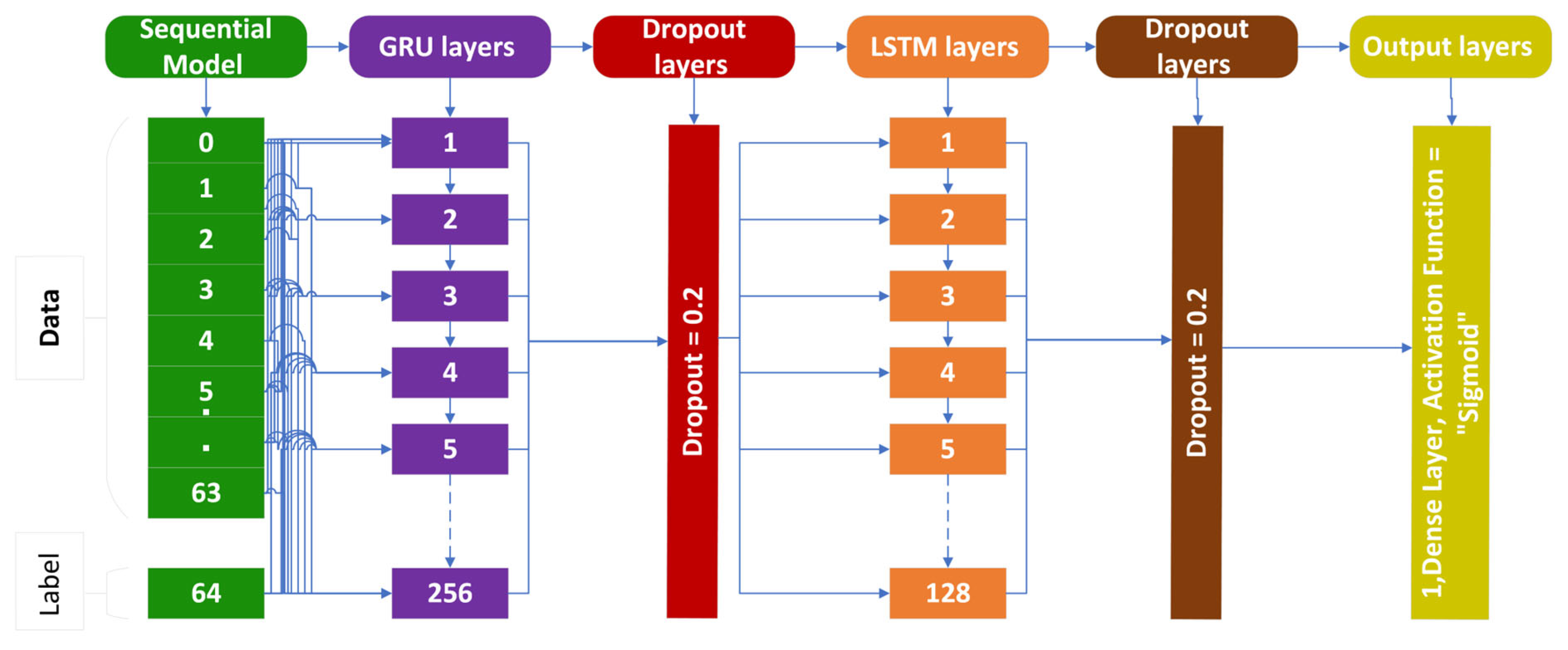
3.2. Gated Recurrent Unit (GRU)
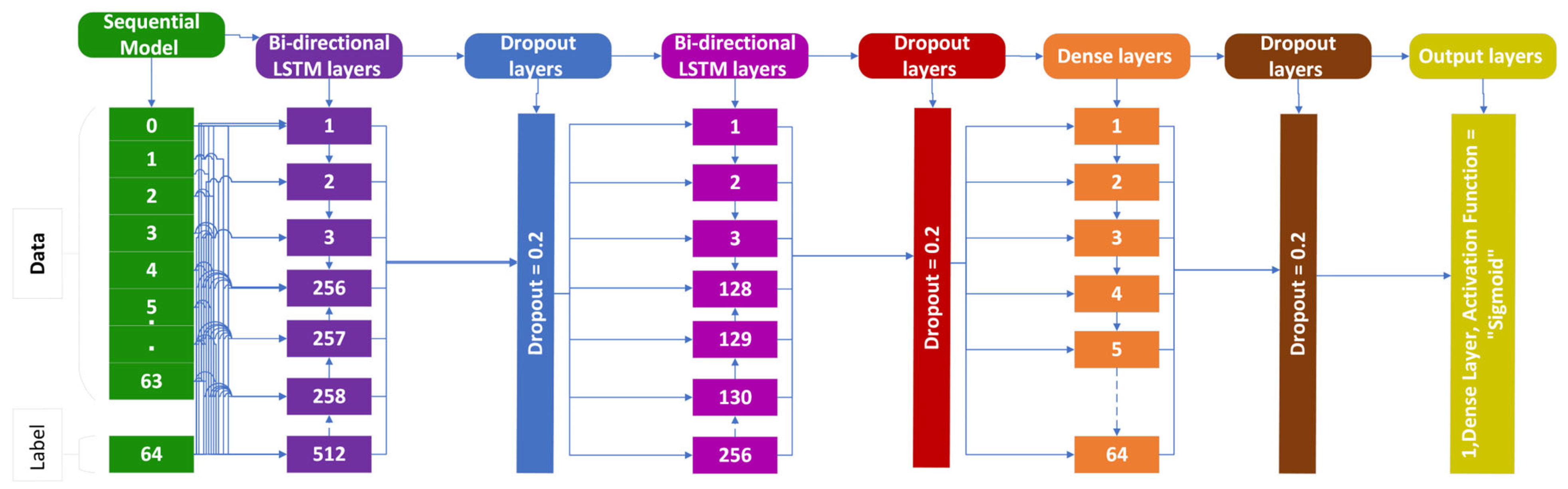
3.3. Bi-Directional LSTM (BLSTM)
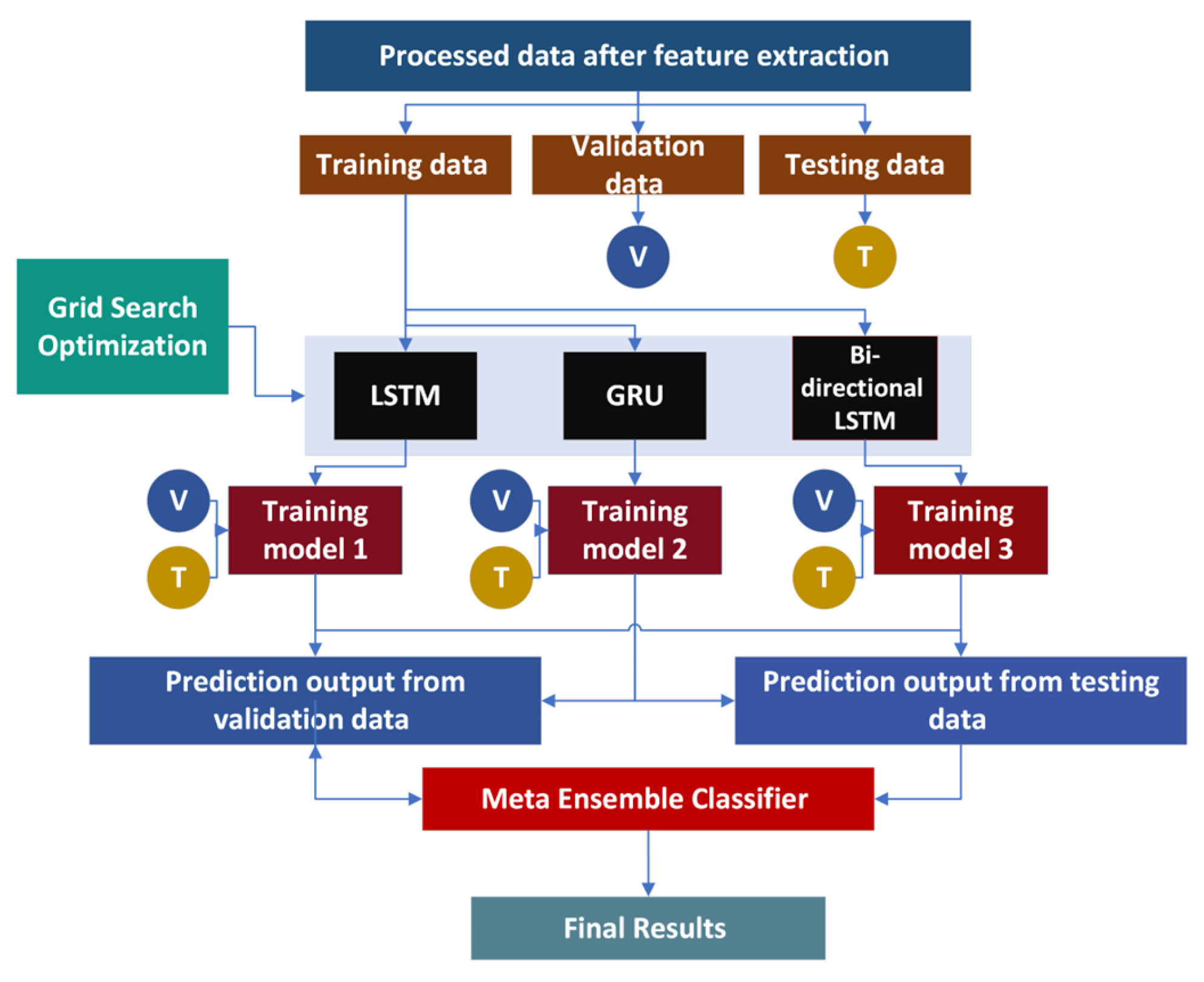
4. Ensemble Deep Learning Models (EDLM)
5. Results
5.1. Self-Consistency Test (SCT)
5.2. Independent Set Test (IST)
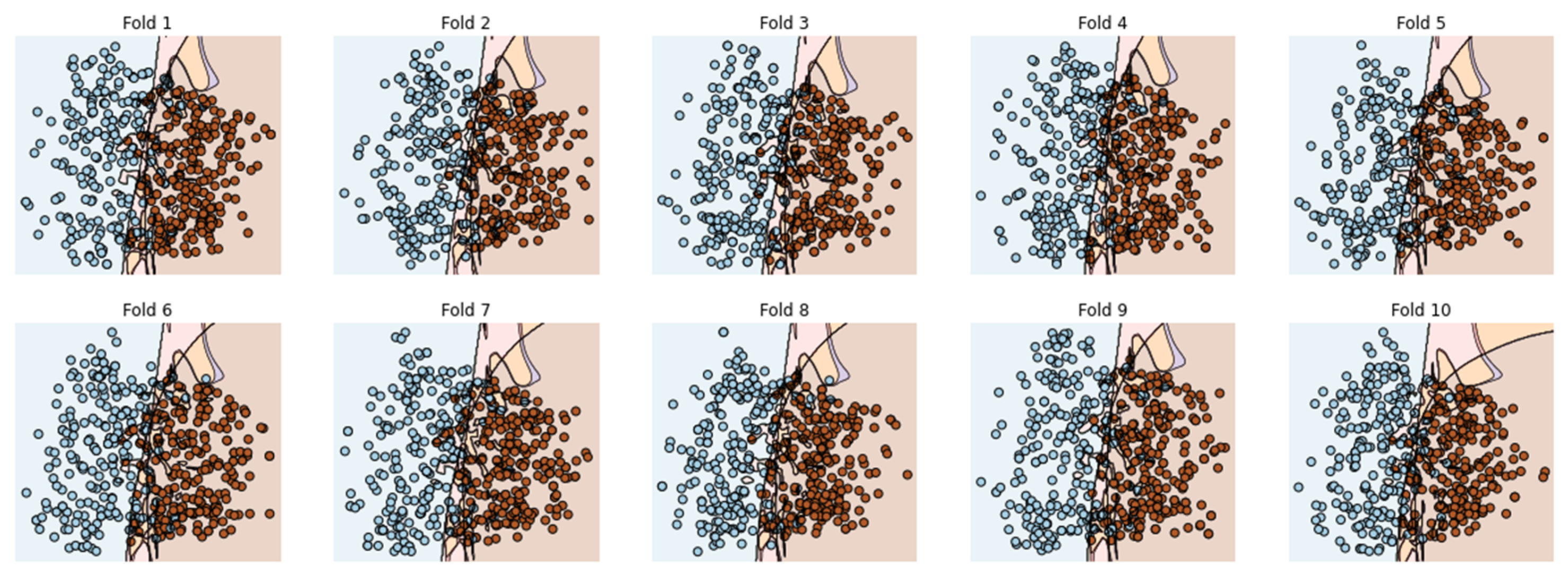
5.3. 10-Fold Cross-Validation (10-FCVT)
5.4. Results Comparison
6. Discussion
7. Conclusions
Author Contributions
Funding
Informed Consent Statement
Acknowledgments
Conflicts of Interest
References
- Hulsen, T.; Jamuar, S.S.; Moody, A.R.; Karnes, J.H.; Varga, O.; Hedensted, S.; Spreafico, R.; Hafler, D.A.; McKinney, E.F. From big data to precision medicine. Front. Med. 2019, 6, 34. [Google Scholar] [CrossRef] [PubMed]
- Haghbin, H.; Aziz, M. Artificial intelligence and cholangiocarcinoma: Updates and prospects. World J. Clin. Oncol. 2022, 13, 125–134. [Google Scholar] [CrossRef] [PubMed]
- Sirica, A.E.; Gores, G.J.; Groopman, J.D.; Selaru, F.M.; Strazzabosco, M.; Wang, X.W.; Zhu, A.X. Intrahepatic Cholangiocarcinoma: Continuing Challenges and Translational Advances. Hepatology 2019, 69, 1803–1815. [Google Scholar] [CrossRef] [PubMed]
- Patel, T. Cholangiocarcinoma-controversies and challenges. Nat. Rev. Gastroenterol. Hepatol. 2011, 8, 189–200. [Google Scholar] [CrossRef]
- Yao, X.; Huang, X.; Yang, C.; Hu, A.; Zhou, G.; Ju, M.; Lei, J.; Shu, J. A novel approach to assessing differentiation degree and lymph node metastasis of extrahepatic cholangiocarcinoma: Prediction using a radiomics-based particle swarm optimization and support vector machine model. JMIR Med. Inform. 2020, 8, e23578. [Google Scholar] [CrossRef]
- Petrick, J.L.; Yang, B.; Altekruse, S.F.; Van Dyke, A.L.; Koshiol, J.; Graubard, B.I.; McGlynn, K.A. Risk factors for intrahepatic and extrahepatic cholangiocarcinoma in the United States: A population-based study in SEER-Medicare. PLoS ONE 2017, 12, e0186643. [Google Scholar] [CrossRef]
- Horgan, A.M.; Amir, E.; Walter, T.; Knox, J.J. Adjuvant therapy in the treatment of biliary tract cancer: A systematic review and meta-analysis. J. Clin. Oncol. 2012, 30, 1934–1940. [Google Scholar] [CrossRef]
- Malaguarnera, G.; Paladina, I.; Giordano, M.; Malaguarnera, M.; Bertino, G.; Berretta, M. Serum markers of intrahepatic cholangiocarcinoma. Dis. Markers 2013, 34, 219–228. [Google Scholar] [CrossRef]
- Bi, Q.; Goodman, K.E.; Kaminsky, J.; Lessler, J. What is machine learning? A primer for the epidemiologist. Am. J. Epidemiol. 2019, 188, 2222–2239. [Google Scholar] [CrossRef]
- Saha, S.K.; Zhu, A.X.; Fuchs, C.S.; Brooks, G.A. Forty-Year Trends in Cholangiocarcinoma Incidence in the U.S.: Intrahepatic Disease on the Rise. Oncologist 2016, 21, 594–599. [Google Scholar] [CrossRef]
- Khan, A.S.; Dageforde, L.A. Cholangiocarcinoma. Surg. Clin. N. Am. 2019, 99, 315–335. [Google Scholar] [CrossRef] [PubMed]
- Tyson, G.L.; El-Serag, H.B. Risk factors for cholangiocarcinoma. Hepatology 2011, 54, 173–184. [Google Scholar] [CrossRef] [PubMed]
- Beretta, G.D.; Robertolabianca, B.; Zampino, M.G.; Gemmagatta, C.; Volkerheinemann, D. Cholangiocarcinoma. Crit. Rev. Oncol. Hematol. 2009, 69, 259–270. [Google Scholar] [CrossRef]
- Matake, K.; Yoshimitsu, K.; Kumazawa, S.; Higashida, Y.; Irie, H.; Asayama, Y.; Nakayama, T.; Kakihara, D.; Katsuragawa, S.; Doi, K.; et al. Usefulness of Artificial Neural Network for Differential Diagnosis of Hepatic Masses on CT Images. Acad. Radiol. 2006, 13, 951–962. [Google Scholar] [CrossRef] [PubMed]
- Logeswaran, R. Cholangiocarcinoma-An automated preliminary detection system using MLP. J. Med. Syst. 2009, 33, 413–421. [Google Scholar] [CrossRef] [PubMed]
- Pattanapairoj, S.; Silsirivanit, A.; Muisuk, K.; Seubwai, W.; Cha’On, U.; Vaeteewoottacharn, K.; Sawanyawisuth, K.; Chetchotsak, D.; Wongkham, S. Improve Discrimination Power of Serum Markers for Diagnosis of Cholangiocarcinoma Using Data Mining-Based Approach; Elsevier: Amsterdam, The Netherlands, 2015; Available online: https://www.sciencedirect.com/science/article/pii/S0009912015001204 (accessed on 16 October 2022).
- Shao, F.; Huang, Q.; Wang, C.; Qiu, L.; Hu, Y.G.; Zha, S.Y. Artificial neural networking model for the prediction of early occlusion of bilateral plastic stent placement for inoperable hilar cholangiocarcinoma. Surg. Laparosc. Endosc. Percutaneous Tech. 2018, 28, e54–e58. Available online: https://www.ingentaconnect.com/content/wk/slept/2018/00000028/00000002/art00004 (accessed on 16 October 2022). [CrossRef]
- Peng, Y.-T.; Zhou, C.-Y.; Lin, P.; Wen, D.-Y.; Wang, X.-D.; Zhong, X.-Z.; Pan, D.-H.; Que, Q.; Li, X.; Chen, L.; et al. Preoperative Ultrasound Radiomics Signatures for Noninvasive Evaluation of Biological Characteristics of Intrahepatic Cholangiocarcinoma. Acad. Radiol. 2020, 27, 785–797. [Google Scholar] [CrossRef]
- Yang, C.; Huang, M.; Li, S.; Chen, J.; Yang, Y.; Qin, N.; Huang, D.; Shu, J. Radiomics Model of Magnetic Resonance Imaging for Predicting Pathological Grading and Lymph Node Metastases of Extrahepatic Cholangiocarcinoma; Elsevier: Amsterdam, The Netherlands, 2020; Available online: https://www.sciencedirect.com/science/article/pii/S0304383519305919 (accessed on 16 October 2022).
- Razumilava, N.; Gores, G.J. Classification, Diagnosis, and Management of Cholangiocarcinoma; Elsevier: Amsterdam, The Netherlands, 2013; Available online: https://www.sciencedirect.com/science/article/pii/S1542356512010506 (accessed on 17 October 2022).
- Vazhayil, A.; KP, S. DeepProteomics: Protein family classification using Shallow and Deep Networks. arXiv 2018, arXiv:1809.04461. [Google Scholar]
- Turecek, D.; Holy, T.; Jakubek, J.; Pospisil, S.; Vykydal, Z. PixEDLMan: A multi-platform data acquisition and processing software package for Medipix2, Timepix and Medipix3 detectors. J. Instrum. 2011, 6, C01046. [Google Scholar] [CrossRef]
- Bozic, I.; Antal, T.; Ohtsuki, H.; Carter, H.; Kim, D.; Chen, S.; Karchin, R.; Kinzler, K.W.; Vogelstein, B.; Nowak, M.A. Accumulation of driver and passenger mutations during tumor progression. Proc. Natl. Acad. Sci. USA 2010, 107, 18545–18550. [Google Scholar] [CrossRef]
- Gene: TP53 (ENSG00000141510)-Summary-Homo_Sapiens-Ensembl Genome Browser 108. Available online: http://asia.ensembl.org/Homo_sapiens/Gene/Summary?g=ENSG00000141510;r=17:7661779-7687538 (accessed on 13 November 2022).
- IntOGen-Cancer Driver Mutations in Breast Adenocarcinoma. Available online: https://intogen.org/search?cancer=BRCA (accessed on 13 November 2022).
- Shah, A.A.; Khan, Y.D. Identification of 4-carboxyglutamate residue sites based on position based statistical feature and multiple classification. Sci. Rep. 2020, 10, 16913. [Google Scholar] [CrossRef]
- Levine, M.D. Feature Extraction: A Survey. Proc. IEEE 1969, 57, 1391–1407. [Google Scholar] [CrossRef]
- Ghoraani, B.; Krishnan, S. Time—Frequency Matrix Feature Extraction and Classification of Environmental Audio Signals. IEEE Trans. Audio Speech Lang. Process. 2011, 19, 2197–2209. [Google Scholar] [CrossRef]
- Hall, A.R. Generalized Method of Moments. 2004. Available online: https://books.google.com/books?hl=en&lr=&id=HQVREAAAQBAJ&oi=fnd&pg=PR9&ots=_0NfFCexpL&sig=21Uxpib37-Wz4QhTV1BowcdVcJo (accessed on 13 November 2022).
- Zhu, H.; Shu, H.; Zhou, J.; Luo, L.; Coatrieux, J.-L. Image analysis by discrete orthogonal dual Hahn moments. Pattern Recognit. Lett. 2007, 28, 1688–1704. [Google Scholar] [CrossRef]
- Malebary, S.J.; Khan, Y.D. Evaluating machine learning methodologies for identification of cancer driver genes. Sci. Rep. 2021, 11, 12281. [Google Scholar] [CrossRef]
- Sohail, M.U.; Shabbir, J.; Sohil, F. Imputation of missing values by using raw moments. Stat. Transit. New Ser. 2019, 20, 21–40. [Google Scholar] [CrossRef]
- Butt, A.H.; Khan, Y.D. CanLect-Pred: A cancer therapeutics tool for prediction of target cancerlectins using experiential annotated proteomic sequences. IEEE Access 2019, 8, 9520–9531. [Google Scholar] [CrossRef]
- Hochreiter, S. The vanishing gradient problem during learning recurrent neural nets and problem solutions. Int. J. Uncertain. Fuzziness Knowl.-Based Syst. 1998, 6, 107–116. [Google Scholar] [CrossRef]
- Wang, H.; Chen, S.; Xu, F.; Jin, Y.-Q. Application of deep-learning algorithms to MSTAR data. In Proceedings of the 25 IEEE International Geoscience and Remote Sensing Symposium (IGARSS), Milan, Italy, 26–31 July 2015; pp. 3743–3745. [Google Scholar]
- Agnes, S.A.; Anitha, J.; Solomon, A.A. Two-stage lung nodule detection framework using enhanced UNet and convolutional LSTM networks in CT images. Comput. Biol. Med. 2022, 149, 106059. [Google Scholar] [CrossRef]
- Sundermeyer, M.; Schlüter, R.; Ney, H. LSTM neural networks for language modeling. In Proceedings of the Thirteenth Annual Conference of The International Speech Communication Association, Portland, OR, USA, 9–13 September 2012. [Google Scholar]
- Rengasamy, D.; Jafari, M.; Rothwell, B.; Chen, X.; Figueredo, G.P. Deep Learning with Dynamically Weighted Loss Function for Sensor-Based Prognostics and Health Management. Sensors 2020, 20, 723. [Google Scholar] [CrossRef]
- Lin, G.; Shen, W. Research on convolutional neural network based on improved Relu piecewise activation function. Procedia Comput. Sci. 2018, 131, 977–984. [Google Scholar] [CrossRef]
- Staudemeyer, R.C.; Morris, E.R. Understanding LSTM—A tutorial into long short-term memory recurrent neural networks. arXiv 2019, arXiv:1909.09586. [Google Scholar]
- Gao, Y.; Glowacka, D. Deep gate recurrent neural network. In Proceedings of the Asian Conference on Machine Learning, Hamilton, New Zealand, 16–18 November 2016; pp. 350–365. [Google Scholar]
- Dey, R.; Salem, F.M. Gate-variants of gated recurrent unit (GRU) neural networks. In Proceedings of the 2017 IEEE 60th International Midwest Symposium on Circuits and Systems (MWSCAS), Boston, MA, USA, 6–9 August 2017; pp. 1597–1600. [Google Scholar]
- Guo, H.; Tang, R.; Ye, Y.; Li, Z.; He, X.; Dong, Z. Deepfm: An end-to-end wide & deep learning framework for CTR prediction. arXiv 2018, arXiv:1804.04950. [Google Scholar]
- Graves, A.; Schmidhuber, J. Framewise phoneme classification with bidirectional LSTM and other neural network architectures. Neural Netw. 2005, 18, 602–610. [Google Scholar] [CrossRef] [PubMed]
- Basaldella, M.; Antolli, E.; Serra, G.; Tasso, C. Bidirectional lstm recurrent neural network for keyphrase extraction. In Proceedings of the Italian Research Conference on Digital Libraries, Udine, Italy, 25–26 January 2018; pp. 180–187. [Google Scholar]
- Mendes-Moreira, J.; Soares, C.; Jorge, A.M.; de Sousa, J.F. Ensemble approaches for regression: A survey. Acm Comput. Surv. 2012, 45, 1–40. [Google Scholar] [CrossRef]
- Breiman, L. Bagging predictors. Mach Learn 1996, 24, 123–140. [Google Scholar] [CrossRef]
- Schapire, R.E. The strength of weak learnability. Mach Learn 1990, 5, 197–227. [Google Scholar] [CrossRef]
- Stefenon, S.F.; Ribeiro, M.H.D.M.; Nied, A.; Mariani, V.C.; Coelho, L.D.S.; Leithardt, V.R.Q.; Silva, L.A.; Seman, L.O. Hybrid wavelet stacking ensemble model for insulators contamination forecasting. IEEE Access 2021, 9, 66387–66397. [Google Scholar] [CrossRef]
- Shah, A.A.; Malik, H.A.M.; Mohammad, A.; Khan, Y.D.; Alourani, A. Machine Learning Techniques for Identification of Carcinogenic Mutations, Which Cause Breast Adenocarcinoma. Sci. Rep. 2022, 12, 11738. [Google Scholar] [CrossRef]
- Shah, A.A.; Alturise, F.; Alkhalifah, T.; Khan, Y.D. Deep Learning Approaches for Detection of Breast Adenocarcinoma Causing Carcinogenic Mutations. Int. J. Mol. Sci. 2022, 23, 11539. [Google Scholar] [CrossRef]
- Shah, A.A.; Alturise, F.; Alkhalifah, T.; Khan, Y.D. Evaluation of Deep Learning Techniques for Identification of Sarcoma-Causing Carcinogenic Mutations. Digit. Health 2022, 8, 20552076221133703. [Google Scholar] [CrossRef] [PubMed]
- Sohail, A.; Nawaz, N.A.; Shah, A.A.; Rasheed, S.; Ilyas, S.; Ehsan, M.K. A Systematic Literature Review on Machine Learning and Deep Learning Methods for Semantic Segmentation. IEEE Access 2022, 10, 134557–134570. [Google Scholar] [CrossRef]
- Shah, A.A.; Malik, H.A.M.; Muhammad, A.; Alourani, A.; Butt, Z.A. Deep Learning Ensemble 2D CNN Approach towards the Detection of Lung Cancer. Sci. Rep. 2023, 13, 2987. [Google Scholar] [CrossRef]
- Amanat, S.; Ashraf, A.; Hussain, W.; Rasool, N.; Khan, Y.D. Identification of Lysine Carboxylation Sites in Proteins by Integrating Statistical Moments and Position Relative Features via General PseAAC. Biomolecules 2020, 10, 396–407. [Google Scholar] [CrossRef]
- Hussain, W.; Rasool, N.; Khan, Y.D. Insights into Machine Learning-Based Approaches for Virtual Screening in Drug Discovery: Existing Strategies and Streamlining through FP-CADD. Molecules 2021, 26, 463–472. [Google Scholar] [CrossRef]
- Hussain, W.; Rasool, N.; Khan, Y.D.; Screening, H.T. A Sequence-Based Predictor of Zika Virus Proteins Developed by Integration of PseAAC and Statistical Moments. Int. J. Environ. Res. Public Health 2020, 17, 797–804. [Google Scholar] [CrossRef]
- Khan, Y.D.; Alzahrani, E.; Alghamdi, W.; Ullah, M.Z. Sequence-Based Identification of Allergen Proteins Developed by Integration of PseAAC and Statistical Moments via 5-Step Rule. Biomolecules 2020, 10, 1046–1055. [Google Scholar] [CrossRef]
- Mahmood, M.K.; Ehsan, A.; Khan, Y.D.; Chou, K.-C. iHyd-LysSite (EPSV): Identifying Hydroxylysine Sites in Protein Using Statistical Formulation by Extracting Enhanced Position and Sequence Variant Feature Technique. Cells 2020, 9, 536–545. [Google Scholar] [CrossRef]
- Naseer, S.; Hussain, W.; Khan, Y.D.; Rasool, N. Optimization of Serine Phosphorylation Prediction in Proteins by Comparing Human Engineered Features and Deep Representations. Int. J. Mol. Sci. 2021, 22, 114069. [Google Scholar] [CrossRef]
- Naseer, S.; Hussain, W.; Khan, Y.D.; Rasool, N. Sequence-Based Identification of Arginine Amidation Sites in Proteins Using Deep Representations of Proteins and PseAAC. Biomolecules 2020, 10, 937–948. [Google Scholar] [CrossRef]
- Naseer, S.; Hussain, W.; Khan, Y.D.; Rasool, N. NPalmitoylDeep-PseAAC: A Predictor of N-Palmitoylation Sites in Proteins Using Deep Representations of Proteins and PseAAC via Modified 5-Steps Rule. Int. J. Mol. Sci. 2021, 22, 294–305. [Google Scholar] [CrossRef]
- Naseer, S.; Hussain, W.; Khan, Y.D.; Rasool, N. iPhosS (Deep)-PseAAC: Identify Phosphoserine Sites in Proteins Using Deep Learning on General Pseudo Amino Acid Compositions via Modified 5-Steps Rule. Bioinformatics 2020, 36, 5709–5711. [Google Scholar] [CrossRef] [PubMed]
- Feng, P.; Yang, H.; Ding, H.; Lin, H.; Chen, W.; Chou, K.-C. iDNA6mA-PseKNC: Identifying DNA N6-methyladenosine sites by incorporating nucleotide physicochemical properties into PseKNC. Genomics 2019, 111, 96–102. [Google Scholar] [CrossRef] [PubMed]
- Hoo, Z.H.; Candlish, J.; Teare, D. What is an ROC curve? Emerg. Med. J. 2017, 34, 357–359. [Google Scholar] [CrossRef] [PubMed]


| Author | Methods | Area Under the Curve |
|---|---|---|
| Matake, et al. [14] | ANN | 0.961 |
| Logeswaran [15] | MLP | 0.960 |
| Pattanapairoj, et al. [16] | C4.5, ANN | 0.961 |
| Shao, et al. [17] | BP-ANN | 0.9648 |
| Peng, et al. [18] | LASSO, SVM | 0.930 |
| Yang, et al. [19] | Random Forest | 0.90 |
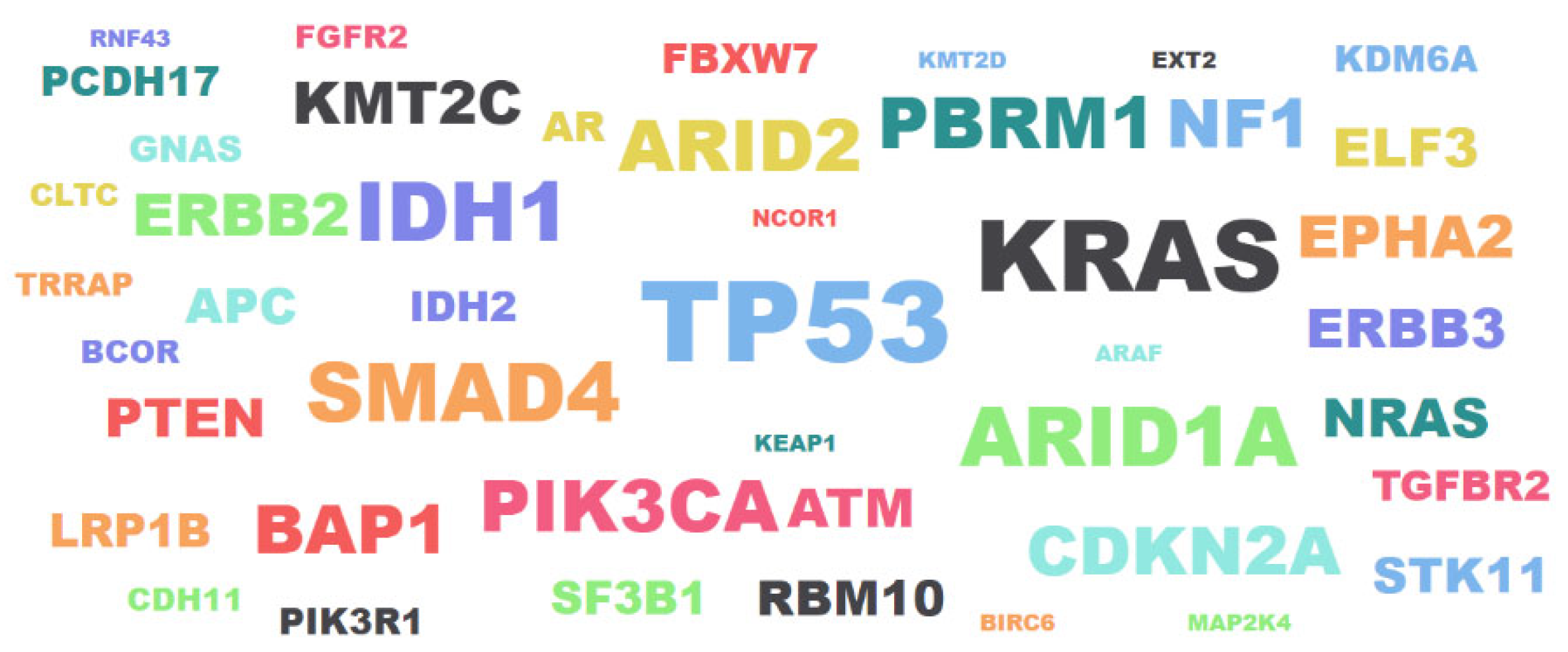
| Symbol | Mutations | Samples | Symbol | Mutations | Samples |
|---|---|---|---|---|---|
| TP53 | 98 | 96 | SF3B1 | 13 | 6 |
| KRAS | 65 | 61 | LRP1B | 26 | 6 |
| ARID1A | 28 | 30 | IDH2 | 5 | 5 |
| SMAD4 | 24 | 28 | TGFBR2 | 5 | 5 |
| IDH1 | 28 | 26 | AR | 9 | 5 |
| PIK3CA | 21 | 19 | PCDH17 | 6 | 5 |
| ARID2 | 21 | 18 | FBXW7 | 8 | 5 |
| PBRM1 | 19 | 18 | GNAS | 11 | 4 |
| BAP1 | 26 | 16 | KDM6A | 6 | 4 |
| CDKN2A | 15 | 15 | PIK3R1 | 5 | 4 |
| NF1 | 17 | 14 | CDH11 | 8 | 3 |
| KMT2C | 17 | 11 | TRRAP | 7 | 3 |
| ERBB2 | 13 | 10 | BCOR | 5 | 3 |
| EPHA2 | 16 | 10 | FGFR2 | 8 | 3 |
| ERBB3 | 14 | 9 | CLTC | 8 | 3 |
| ATM | 18 | 9 | KEAP1 | 1 | 2 |
| ELF3 | 9 | 9 | NCOR1 | 2 | 2 |
| NRAS | 10 | 8 | ARAF | 3 | 2 |
| PTEN | 9 | 8 | KMT2D | 16 | 2 |
| APC | 13 | 7 | EXT2 | 3 | 2 |
| STK11 | 9 | 7 | MAP2K4 | 2 | 2 |
| RBM10 | 12 | 7 | BIRC6 | 11 | 2 |
| RNF43 | 2 | 2 |
| Self-Consistency Test (SCT) | Independent Set Test (IST) | 10-Fold Cross-Validation Test (10-FCVT) | ||||||||||
|---|---|---|---|---|---|---|---|---|---|---|---|---|
| Acc | Sn | Sp | MCC | Acc | Sn | Sp | MCC | Acc | Sn | Sp | MCC | |
| LSTM | 94% | 97% | 93% | 0.89 | 93% | 95% | 91% | 0.87 | 92% | 91% | 93% | 0.85 |
| GRU | 94% | 95% | 93% | 0.88 | 94% | 96% | 92% | 0.89 | 92% | 91% | 93% | 0.84 |
| BLSTM | 99% | 100% | 98% | 0.98 | 98% | 100% | 96% | 0.95 | 92% | 91% | 93% | 0.84 |
| EDLM | 94% | 95% | 93% | 0.88 | 96% | 98% | 94% | 0.92 | 92% | 94% | 93% | 0.86 |
| Previous Results | ||
|---|---|---|
| Author | Models | Area Under the Curve |
| Matake, et al. [14] | ANN | 0.961 |
| Logeswaran [15] | MLP | 0.960 |
| Pattanapairoj, et al. [16] | C4.5, ANN | 0.961 |
| Shao, et al. [17] | BP-ANN | 0.9648 |
| Peng, et al. [18] | LASSO, SVM | 0.930 |
| Yang, et al. [19] | Random Forest | 0.90 |
| Proposed Results | ||
| Models | Area Under the Curve | |
| LSTM | 0.98 | |
| GRU | 0.97 | |
| BLSTM | 0.99 | |
| EDLM | 0.98 | |
| Evaluation Matrices | Values | Evaluation Matrices | Values |
|---|---|---|---|
| Accuracy | 98.87% | Precision | 98.87% |
| Sensitivity | 99.50% | Recall | 98.87% |
| Specificity | 99.63% | F1 Score | 98.87% |
| MCC | 0.98 | AUC | 0.99 |
Disclaimer/Publisher’s Note: The statements, opinions and data contained in all publications are solely those of the individual author(s) and contributor(s) and not of MDPI and/or the editor(s). MDPI and/or the editor(s) disclaim responsibility for any injury to people or property resulting from any ideas, methods, instructions or products referred to in the content. |
© 2023 by the authors. Licensee MDPI, Basel, Switzerland. This article is an open access article distributed under the terms and conditions of the Creative Commons Attribution (CC BY) license (https://creativecommons.org/licenses/by/4.0/).
Share and Cite
Shah, A.A.; Alturise, F.; Alkhalifah, T.; Faisal, A.; Khan, Y.D. EDLM: Ensemble Deep Learning Model to Detect Mutation for the Early Detection of Cholangiocarcinoma. Genes 2023, 14, 1104. https://doi.org/10.3390/genes14051104
Shah AA, Alturise F, Alkhalifah T, Faisal A, Khan YD. EDLM: Ensemble Deep Learning Model to Detect Mutation for the Early Detection of Cholangiocarcinoma. Genes. 2023; 14(5):1104. https://doi.org/10.3390/genes14051104
Chicago/Turabian StyleShah, Asghar Ali, Fahad Alturise, Tamim Alkhalifah, Amna Faisal, and Yaser Daanial Khan. 2023. "EDLM: Ensemble Deep Learning Model to Detect Mutation for the Early Detection of Cholangiocarcinoma" Genes 14, no. 5: 1104. https://doi.org/10.3390/genes14051104