
Comparing Genetic and Physical Anthropological Analyses for the Biological Profile of Unidentified and Identified Bodies in Milan
 , , ,
, , ,
Abstract
:1. Introduction
2. Materials and Methods
2.1. Sample
2.2. Physical Analyses
2.3. Molecular Analyses
2.3.1. Parma Forensic Biological Unit of Carabinieri
- Sample Inspection and Processing
- STR Loci Amplification: Autosomal DNA and Y Chromosome Markers
- Typing of Both Autosomal and Y-Chromosome Markers
2.3.2. Forensic Molecular Anthropology Laboratory (Florence)
- Sample Preparation and DNA Extraction
- Library Preparation, Enrichment and Data Processing
- Statistical Analysis
3. Result and Discussion
3.1. Physical Results
3.2. Molecular Results
3.2.1. Autosomal and Y STRs
3.2.2. Mitochondrial DNA
3.3. PLS-DA Results
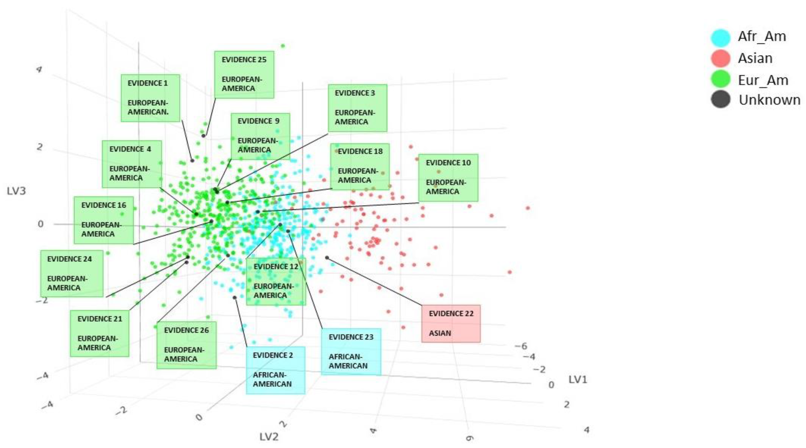
3.3.1. Autosomal STRs
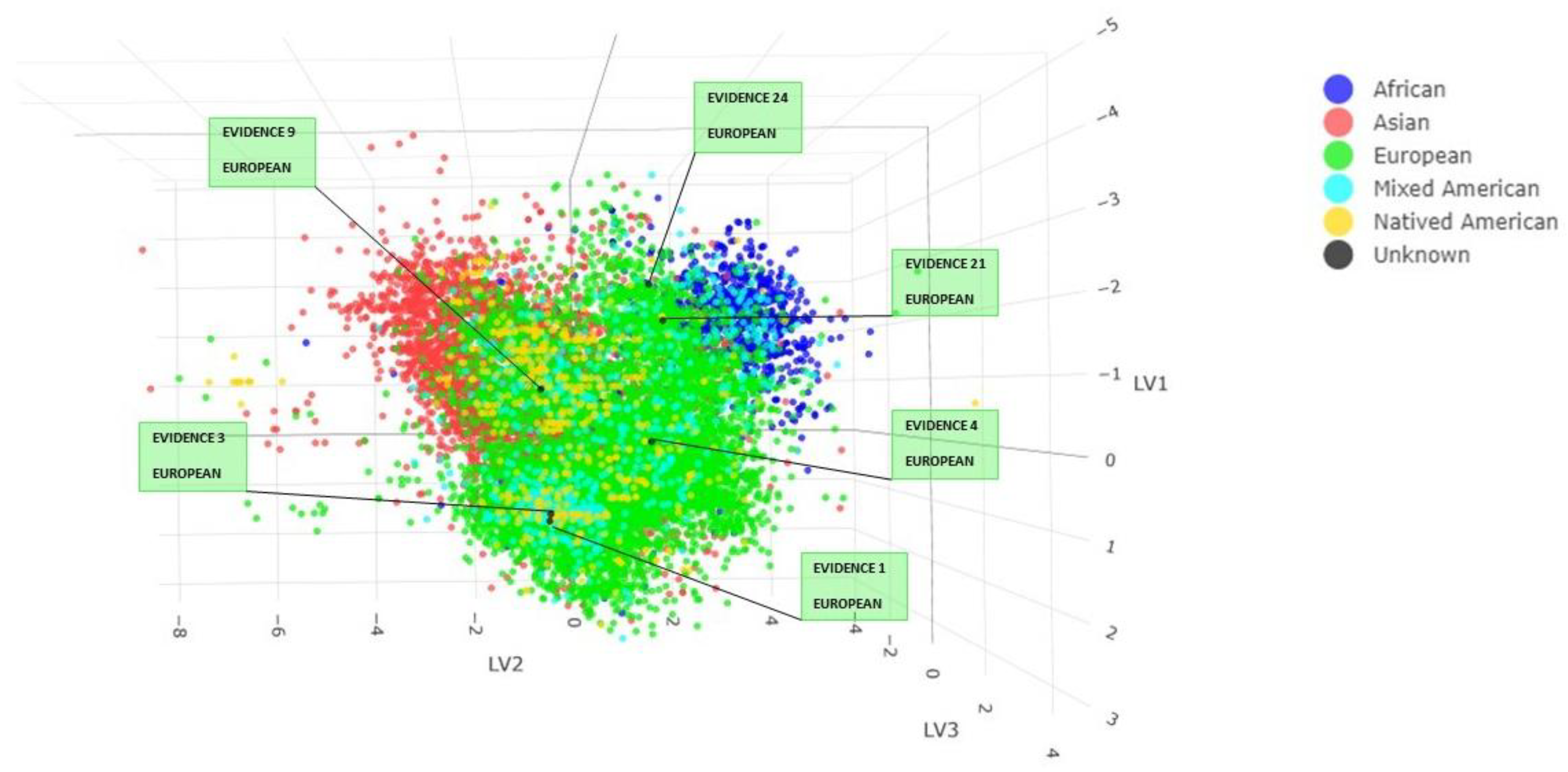
3.3.2. Y STRs
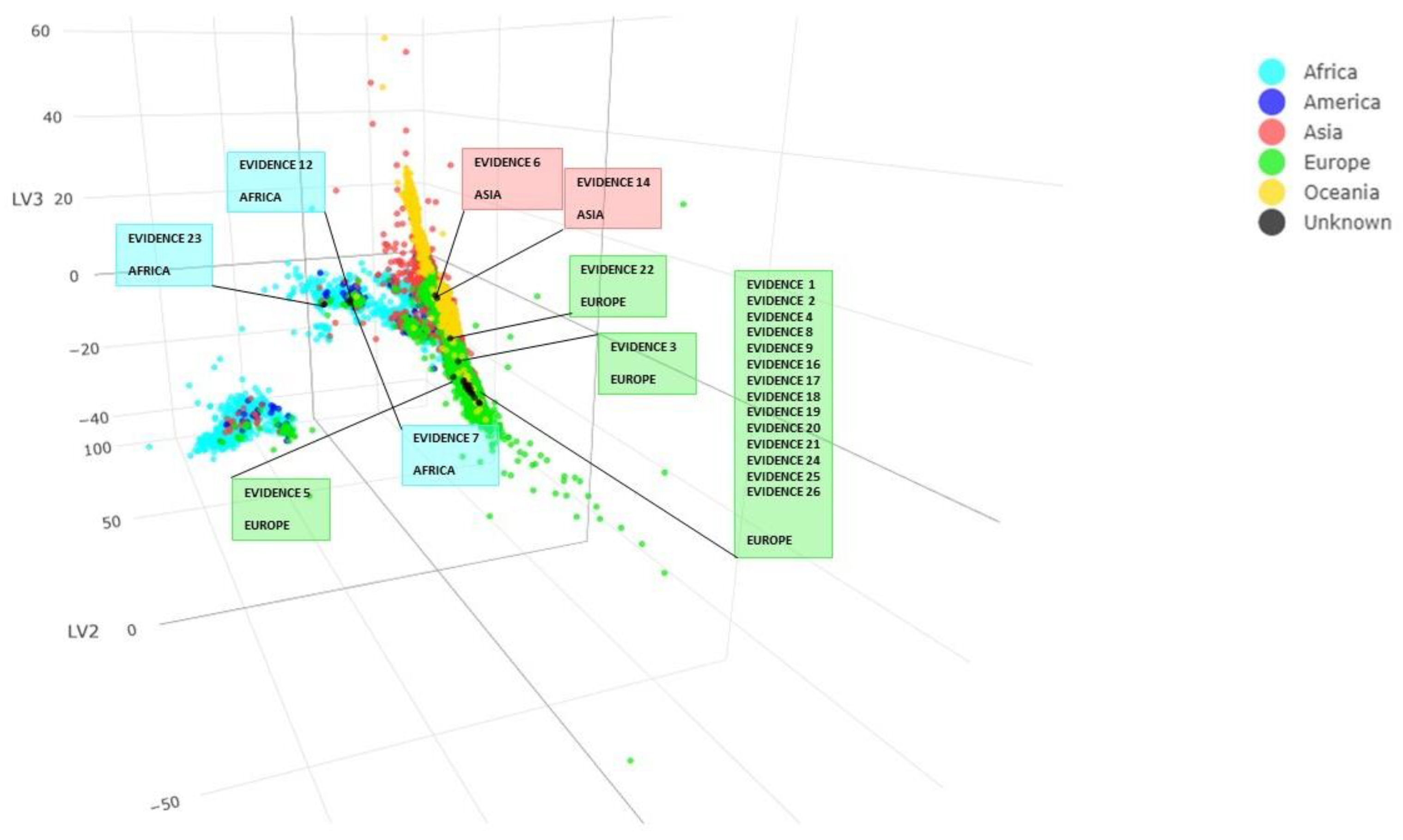
3.3.3. mtDNA
3.4. Mirroring Physical and Genetic Results
4. Conclusions
Supplementary Materials
Author Contributions
Funding
Institutional Review Board Statement
Informed Consent Statement
Data Availability Statement
Conflicts of Interest
References
- Klales, A.R. Practitioner preferences for sex estimation from human skeletal remains. In Sex Estimation of the Human Skeleton; Elsevier: Amsterdam, The Netherlands, 2020; pp. 11–23. [Google Scholar]
- Phenice, T.W. A newly developed visual method of sexing the os pubis. Am. J. Phys. Anthropol. 1969, 30, 297–301. [Google Scholar] [CrossRef]
- Cappella, A.; Bertoglio, B.; Di Maso, M.; Mazzarelli, D.; Affatato, L.; Stacchiotti, A.; Sforza, C.; Cattaneo, C. Sexual Dimorphism of Cranial Morphological Traits in an Italian Sample: A Population-Specific Logistic Regression Model for Predicting Sex. Biology 2022, 11, 1202. [Google Scholar] [CrossRef] [PubMed]
- Walker, P.L. Sexing skulls using discriminant function analysis of visually assessed traits. Am. J. Phys. Anthropol. 2008, 136, 39–50. [Google Scholar] [CrossRef] [PubMed]
- Spradley, M.K.; Jantz, R.L. Sex estimation in forensic anthropology: Skull versus postcranial elements. J. Forensic Sci. 2011, 56, 289–296. [Google Scholar] [CrossRef] [PubMed]
- Bass, W.M. Human Osteology: A Laboratory and Field Manual, 4th ed.; Eborn Books: Salt Lake City, UT, USA, 1995. [Google Scholar]
- Hefner, J.T. Cranial nonmetric variation and estimating ancestry. J. Forensic Sci. 2009, 54, 985–995. [Google Scholar] [CrossRef] [PubMed]
- Gill, G.W. Craniofacial criteria in the skeletal attribution of race. In Forensic Osteology: Advances in the Identification of Human Remains; Reichs, K.J., Ed.; Charles C Thomas: Springfield, IL, USA, 1998; pp. 293–315. ISBN 97803980-68042. [Google Scholar]
- Ousley, S.D.; Jantz, R.L. Fordisc 3 and Statistical Methods for Estimating Sex and Ancestry. In A Companion to Forensic Anthropol; Blackwell Publishing Ltd.: Hoboken, NJ, USA, 2012; pp. 311–329. [Google Scholar] [CrossRef]
- Dumache, R.; Ciocan, V.; Muresan, C.; Enache, A. Molecular DNA Analysis in Forensic Identification. Clin. Lab. 2016, 62, 245–248. [Google Scholar] [CrossRef] [PubMed]
- Afrifah, K.; Badu-Boateng, A.; Antwi-Akomeah, S.; Motey, E.; Boampong, E.; Twumasi, P.; Sampene, P.; Donkor, A. Forensic identification of missing persons using DNA from surviving relatives and femur bone retrieved from salty environment. J. Forensic Sci. Med. 2020, 6, 40. [Google Scholar] [CrossRef]
- Leclair, B.; Shaler, R.; Carmody, G.R.; Eliason, K.; Hendrickson, B.C.; Judkins, T.; Norton, M.J.; Sears, C.; Scholl, T. Bioinformatics and human identification in mass fatality incidents: The World Trade Center disaster. J. Forensic Sci. 2007, 52, 806–819. [Google Scholar] [CrossRef]
- Yang, J.; Chen, J.; Ji, Q.; Li, K.; Deng, C.; Kong, X.; Xie, S.; Zhan, W.; Mao, Z.; Zhang, B.; et al. Could routine forensic STR genotyping data leak personal phenotypic information? Forensic Sci. Int. 2022, 335, 111311. [Google Scholar] [CrossRef]
- Alladio, E.; Della Rocca, C.; Barni, F.; Dugoujon, J.-M.; Garofano, P.; Semino, O.; Berti, A.; Novelletto, A.; Vincenti, M.; Cruciani, F. A multivariate statistical approach for the estimation of the ethnic origin of unknown genetic profiles in forensic genetics. Forensic Sci. Int. Genet. 2020, 45, 102209. [Google Scholar] [CrossRef]
- Thomas, R.M.; Parks, C.L.; Richard, A.H. Accuracy Rates of Sex Estimation by Forensic Anthropologists through Comparison with DNA Typing Results in Forensic Casework. J. Forensic Sci. 2016, 61, 1307–1310. [Google Scholar] [CrossRef] [PubMed]
- Thomas, R.M.; Parks, C.L.; Richard, A.H. Accuracy Rates of Ancestry Estimation by Forensic Anthropologists Using Identified Forensic Cases. J. Forensic Sci. 2017, 62, 971–974. [Google Scholar] [CrossRef] [PubMed]
- Mazzarelli, D.; Milotta, L.; Franceschetti, L.; Maggioni, L.; Merelli, V.G.; Poppa, P.; Porta, D.; De Angelis, D.; Cattaneo, C. Twenty-five years of unidentified bodies: An account from Milano, Italy. Int. J. Legal Med. 2021, 135, 1983–1991. [Google Scholar] [CrossRef] [PubMed]
- Buikstra, J.E.; Ubelaker, D.H. Standards for Data Collection from Human Skeletal Remains. Arkansas Archeological Survey Research Series No. 44. Plains Anthropol. 1994, 41, 197–200. [Google Scholar]
- Brooks, S.; Suchey, J.M. Skeletal age determination based on the os pubis: A comparison of the Acsádi-Nemeskéri and Suchey-Brooks methods. Hum. Evol. 1990, 5, 227–238. [Google Scholar] [CrossRef]
- Işcan, M.Y.; Loth, S.R. Determination of Age from the Sternal Rib in White Males: A Test of the Phase Method. J. Forensic Sci. 1986, 31, 11866J. [Google Scholar] [CrossRef]
- İşcan, M.Y.; Loth, S.R. Determination of Age from the Sternal Rib in White Females: A Test of the Phase Method. J. Forensic Sci. 1986, 31, 11107J. [Google Scholar] [CrossRef]
- Lovejoy, C.O.; Meindl, R.S.; Mensforth, R.P.; Barton, T.J. Multifactorial determination of skeletal age at death: A method and blind tests of its accuracy. Am. J. Phys. Anthropol. 1985, 68, 1–14. [Google Scholar] [CrossRef]
- Kvaal, S.I.; Kolltveit, K.M.; Thomsen, I.O.; Solheim, T. Age estimation of adults from dental radiographs. Forensic Sci. Int. 1995, 74, 175–185. [Google Scholar] [CrossRef]
- Lamendin, H.; Baccino, E.; Humbert, J.F.; Tavernier, J.C.; Nossintchouk, R.M.; Zerilli, A. A simple technique for age estimation in adult corpses: The two criteria dental method. J. Forensic Sci. 1992, 37, 1373–1379. [Google Scholar] [CrossRef]
- Skinner, R.A.; Hickmon, S.G.; Lumpkin, C.K.; Aronson, J.; Nicholas, R.W. Decalcified Bone: Twenty Years of Successful Specimen Management. J. Histotechnol. 1997, 20, 267–277. [Google Scholar] [CrossRef]
- Callis, G.; Sterchi, D. Decalcification of Bone: Literature Review and Practical Study of Various Decalcifying Agents. Methods, and Their Effects on Bone Histology. J. Histotechnol. 1998, 21, 49–58. [Google Scholar] [CrossRef]
- Butler, J.M. Short tandem repeat typing technologies used in human identity testing. Biotechniques 2007, 43, ii–v. [Google Scholar] [CrossRef] [PubMed]
- Sirak, K.A.; Fernandes, D.M.; Cheronet, O.; Novak, M.; Gamarra, B.; Balassa, T.; Bernert, Z.; Cséki, A.; Dani, J.; Gallina, J.Z.; et al. A minimally-invasive method for sampling human petrous bones from the cranial base for ancient DNA analysis. Biotechniques 2017, 62, 283–289. [Google Scholar] [CrossRef]
- Dabney, J.; Knapp, M.; Glocke, I.; Gansauge, M.-T.; Weihmann, A.; Nickel, B.; Valdiosera, C.; García, N.; Pääbo, S.; Arsuaga, J.-L.; et al. Complete mitochondrial genome sequence of a Middle Pleistocene cave bear reconstructed from ultrashort DNA fragments. Proc. Natl. Acad. Sci. USA 2013, 110, 15758–15763. [Google Scholar] [CrossRef]
- Meyer, M.; Kircher, M. Illumina Sequencing Library Preparation for Highly Multiplexed Target Capture and Sequencing. Cold Spring Harb. Protoc. 2010, 2010, pdb-prot5448. [Google Scholar] [CrossRef]
- Maricic, T.; Whitten, M.; Pääbo, S. Multiplexed DNA sequence capture of mitochondrial genomes using PCR products. PLoS ONE 2010, 5, e14004. [Google Scholar] [CrossRef]
- Peltzer, A.; Jäger, G.; Herbig, A.; Seitz, A.; Kniep, C.; Krause, J.; Nieselt, K. EAGER: Efficient ancient genome reconstruction. Genome Biol. 2016, 17, 60. [Google Scholar] [CrossRef]
- Li, H.; Durbin, R. Fast and accurate short read alignment with Burrows-Wheeler transform. Bioinformatics 2009, 25, 1754–1760. [Google Scholar] [CrossRef]
- Zimek, A.; Schubert, E.; Kriegel, H.-P. A survey on unsupervised outlier detection in high-dimensional numerical data. Stat. Anal. Data Min. 2012, 5, 363–387. [Google Scholar] [CrossRef]
- Jónsson, H.; Ginolhac, A.; Schubert, M.; Johnson, P.L.F.; Orlando, L. MapDamage 2.0: Fast approximate Bayesian estimates of ancient DNA damage parameters. Bioinformatics 2013, 29, 1682–1684. [Google Scholar] [CrossRef] [PubMed]
- Renaud, G.; Slon, V.; Duggan, A.T.; Kelso, J. Schmutzi: Estimation of contamination and endogenous mitochondrial consensus calling for ancient DNA. Genome Biol. 2015, 16, 224. [Google Scholar] [CrossRef]
- Schönherr, S.; Weissensteiner, H.; Kronenberg, F.; Forer, L. Haplogrep 3—An interactive haplogroup classification and analysis platform. Nucleic Acids Res. 2023, gkad284. [Google Scholar] [CrossRef] [PubMed]
- Ruiz-Perez, D.; Guan, H.; Madhivanan, P.; Mathee, K.; Narasimhan, G. So you think you can PLS-DA? BMC Bioinformatics 2020, 21, 2. [Google Scholar] [CrossRef] [PubMed]
- Ståhle, L.; Wold, S. Partial least squares analysis with cross-validation for the two-class problem: A Monte Carlo study. J. Chemom. 1987, 1, 185–196. [Google Scholar] [CrossRef]
- Brereton, R.G.; Lloyd, G.R. Partial least squares discriminant analysis: Taking the magic away. J. Chemom. 2014, 28, 213–225. [Google Scholar] [CrossRef]
- Saccenti, E.; Timmerman, M.E. Approaches to Sample Size Determination for Multivariate Data: Applications to PCA and PLS-DA of Omics Data. J. Proteome Res. 2016, 15, 2379–2393. [Google Scholar] [CrossRef]
- Filzmoser, P.; Liebmann, B.; Varmuza, K. Repeated double cross validation. J. Chemom. 2009, 23, 160–171. [Google Scholar] [CrossRef]
- Hill, C.R.; Duewer, D.L.; Kline, M.C.; Coble, M.D.; Butler, J.M. U.S. population data for 29 autosomal STR loci. Forensic Sci. Int. Genet. 2013, 7, e82–e83. [Google Scholar] [CrossRef]
- Purps, J.; Siegert, S.; Willuweit, S.; Nagy, M.; Alves, C.; Salazar, R.; Angustia, S.M.T.; Santos, L.H.; Anslinger, K.; Bayer, B.; et al. A global analysis of Y-chromosomal haplotype diversity for 23 STR loci. Forensic Sci. Int. Genet. 2014, 12, 12–23. [Google Scholar] [CrossRef]
- Clima, R.; Preste, R.; Calabrese, C.; Diroma, M.A.; Santorsola, M.; Scioscia, G.; Simone, D.; Shen, L.; Gasparre, G.; Attimonelli, M. HmtDB 2016: Data update, a better performing query system and human mitochondrial DNA haplogroup predictor. Nucleic Acids Res. 2017, 45, D698–D706. [Google Scholar] [CrossRef] [PubMed]
- Alladio, E.; Poggiali, B.; Cosenza, G.; Pilli, E. Multivariate statistical approach and machine learning for the evaluation of biogeographical ancestry inference in the forensic field. Sci. Rep. 2022, 12, 8974. [Google Scholar] [CrossRef] [PubMed]
- Pilli, E.; Morelli, S.; Poggiali, B.; Alladio, E. Biogeographical ancestry, variable selection, and PLS-DA method: A new panel to assess ancestry in forensic samples via MPS technology. Forensic Sci. Int. Genet. 2023, 62, 102806. [Google Scholar] [CrossRef] [PubMed]
- Ousley, S.; Jantz, R.; Freid, D. Understanding race and human variation: Why forensic anthropologists are good at identifying race. Am. J. Phys. Anthropol. 2009, 139, 68–76. [Google Scholar] [CrossRef] [PubMed]
- Phillips, C. Forensic genetic analysis of bio-geographical ancestry. Forensic Sci. Int. Genet. 2015, 18, 49–65. [Google Scholar] [CrossRef]
- Pilli, E.; Palamenghi, A.; Morelli, S.; Mazzarelli, D.; De Angelis, D.; Jantz, R.L.; Cattaneo, C. How Physical and Molecular Anthropology Interplay in the Creation of Biological Profiles of Unidentified Migrants. Genes 2023, 14, 706. [Google Scholar] [CrossRef]


| Case ID | Taphonomic Condition | PMI at Recovery | Bone Sampled for Genetics |
|---|---|---|---|
| Evidence 1 | Skeletonized | Few months | Tibia |
| Evidence 2 | Skeletonized | 10 years | Femur |
| Evidence 3 | Skeletonized | 17 years | Femur |
| Evidence 4 | Skeletonized | 17 years | Femur |
| Evidence 5 | Skeletonized | 1–2 years | Femur |
| Evidence 6 | Partially skeletonized, burnt | Few weeks | Tibia |
| Evidence 7 | Skeletonized | Few months | Femur |
| Evidence 8 | Skeletonized | 7 years | Petrous bone |
| Evidence 9 | Partially skeletonized, burnt | 1 week | Femur |
| Evidence 10 | Skeletonized | 20 years | Petrous bone |
| Evidence 12 | Skeletonized | 8 years | Femur |
| Evidence 14 | Skeletonized | 6–12 months | Femur |
| Evidence 15 | Skeletonized | Few months | Femur |
| Evidence 16 | Skeletonized | 1–2 years | Femur |
| Evidence 17 | Adipocere, skeletonized | 6–12 months | Femur |
| Evidence 18 | Skeletonized | 8 months | Petrous bone |
| Evidence 19 | Skeletonized | 3–6 months | Femur |
| Evidence 20 | Skeletonized | 3–6 months | Femur |
| Evidence 21 | Skeletonized | 5–6 months | Femur |
| Evidence 22 | Skeletonized | 3 months–1 year | Petrous bone |
| Evidence 23 | Skeletonized | 1–2 years | Tibia |
| Evidence 24 | Skeletonized, partially burnt | 3–7 months | Femur |
| Evidence 25 | Partially skeletonized | 1–2 weeks | Femur |
| Evidence 26 | Skeletonized | 1–3 years | Femur |
| Case ID | Skeletal Sex | Skeletal Ancestry | Age-at-Death Estimation (Years) | Y-DNA Haplogroup Probability Assigned by Nevgen Predictor | mtDNA Haplogroup | Continent |
|---|---|---|---|---|---|---|
| Evidence 1 | M | European | 43–57 | R1b M269—western Europe 100% | H1(H1) | Europe |
| Evidence 2 | M | European | 40–54 | R1b M269—western Europe 100% | U5a(U5a1b1g) | Europe |
| Evidence 3 | M | European | 21–56 | R1b M269—western Europe 99.92% | R0(R0) | South Asian |
| Evidence 4 | M | European | 26–45 | I2a1b3—south-eastern, south-western, north-western Europe 100% | H(H) | Europe |
| Evidence 5 | M | European | 26–45 | ND | U6a(U6a3b) | Europe |
| Evidence 6 | F | European | 30–50 | Female | M5a(M5a1b) | South Asia |
| Evidence 7 | F | African | 18–22 | Female | L2a(L2a1a1) | Africa/Africa America |
| Evidence 8 | M | European | >60 | NA | U4b(U4b1a3a) | Europe |
| Evidence 9 | M | European | 36–50 | J2a1 M67—Europe, the Middle East and northern Africa 96.4% | T2e(T2e2a) | Europe |
| Evidence 10 | IND | European | 18–39 | Female | L3e(L3e1a3a) | Africa/Africa America |
| Evidence 12 | M | European | 35–44 | E1b1b L67–Europe, the Near East, and northern Africa 100% | L2a(L2a1c1) | Africa/Africa America |
| Evidence 14 | F | European | 38–50 | Female | M5a(M5a1b) | South Asia |
| Evidence 15 | F | European | 34–63 | Female | M1a(M1a1) | South Asia |
| Evidence 16 | M | European | 30–44 | I2a1b3—south-eastern, south-western, north-western Europe 100% | T1a(T1a10) | Europe |
| Evidence 17 | M | European | 57–71 | NA | H1b(H1bp) | Europe |
| Evidence 18 | F | European | 17–22 | Female | K1a(K1a) | Europe |
| Evidence 19 | F | European | 30–50 | NA | T2(T2+16189) | Europe |
| Evidence 20 | F | European | 17–22 | Female | H41a(H41a) | Europe |
| Evidence 21 | M | European | 32–52 | E1b1b >V13—Europe, the Near East, and northern Africa 99.92% | H1b(H1b1+16362) | Europe |
| Evidence 22 | F | African | 28–52 | Female | R9c(R9c1b1) | South Asia |
| Evidence 23 | F | African | 37–52 | Female | L2b(L2b1b) | Africa/ Africa America |
| Evidence 24 | M | European | 60–80 | E1b1b >V13—Europe, the Near East, and northern Africa 74.5% | U5a(U5a1c) | Europe |
| Evidence 25 | F | European | 39–53 | Female | J2b(J2b1c) | Europe |
| Evidence 26 | M | European | >60 | R1b—western Europe | K1a(K1a4a1h) | Europe |
| Case ID | Physical Sex | Molecular Sex | Physical Ancestry | Genetic Ancestry | ||
|---|---|---|---|---|---|---|
| STR | Y | MtDNA | ||||
| Evidence 1 | M | M | European | Eur_Am | EU | EU |
| Evidence 2 | M | M | European | Afr_Am | EU | EU |
| Evidence 3 | M | M | European | Eur_Am | EU | EU |
| Evidence 4 | M | M | European | Eur_Am | EU | EU |
| Evidence 5 | M | M | European | NA | ND | EU |
| Evidence 6 | F | F | European | Eur_Am | NA | AS |
| Evidence 7 | F | F | African | Afr_Am | NA | AF |
| Evidence 8 | M | M | European | Eur_Am | NA | EU |
| Evidence 9 | M | M | European | Eur_Am | EU | EU |
| Evidence 10 | IND | F | European | Eur_Am | NA | ND |
| Evidence 12 | M | M | European | Eur_Am | EU | AF |
| Evidence 14 | F | F | European | Eur_Am | NA | AS |
| Evidence 15 | F | F | European | ND | NA | ND |
| Evidence 16 | M | M | European | Eur_Am | EU | EU |
| Evidence 17 | M | ND | European | NA | NA | EU |
| Evidence 18 | F | F | European | Eur_Am | NA | EU |
| Evidence 19 | F | ND | European | NA | NA | EU |
| Evidence 20 | F | F | European | Eur_Am | NA | EU |
| Evidence 21 | M | M | European | Eur_Am | EU | EU |
| Evidence 22 | F | F | African | Asian | NA | EU |
| Evidence 23 | F | F | African | Afr_Am | NA | AF |
| Evidence 24 | M | M | European | Eur_Am | EU | EU |
| Evidence 25 | F | F | European | Eur_Am | NA | EU |
| Evidence 26 | M | M | European | Eur_Am | EU | EU |
| Case ID | Physical Sex | Molecular Sex | Known Sex | Known Provenance | Physical Ancestry | Genetic Ancestry | ||
|---|---|---|---|---|---|---|---|---|
| STR | Y | mtDNA | ||||||
| Evidence 1 | M | M | M | Italy | European | Eur_Am | EU | EU |
| Evidence 2 | M | M | M | Italy | European | Afr_Am | EU | EU |
| Evidence 6 | F | F | F | Ukraine | European | Eur_Am | NA | AS |
| Evidence 7 | F | F | F | Nigeria | African | Afr_Am | NA | AF |
| Evidence 8 | M | M | M | Germany | European | Eur_Am | NA | EU |
| Evidence 9 | M | M | M | Italy | European | Eur_Am | EU | EU |
| Evidence 12 | M | M | M | Morocco | European | Eur_Am | EU | AF |
| Evidence 25 | F | F | F | Italy | European | Eur_Am | NA | EU |
| Evidence 26 | M | M | M | Italy | European | Eur_Am | EU | EU |
Disclaimer/Publisher’s Note: The statements, opinions and data contained in all publications are solely those of the individual author(s) and contributor(s) and not of MDPI and/or the editor(s). MDPI and/or the editor(s) disclaim responsibility for any injury to people or property resulting from any ideas, methods, instructions or products referred to in the content. |
© 2023 by the authors. Licensee MDPI, Basel, Switzerland. This article is an open access article distributed under the terms and conditions of the Creative Commons Attribution (CC BY) license (https://creativecommons.org/licenses/by/4.0/).
Share and Cite
Pilli, E.; Palamenghi, A.; Marino, A.; Staiti, N.; Alladio, E.; Morelli, S.; Cherubini, A.; Mazzarelli, D.; Caccia, G.; Gibelli, D.; et al. Comparing Genetic and Physical Anthropological Analyses for the Biological Profile of Unidentified and Identified Bodies in Milan. Genes 2023, 14, 1064. https://doi.org/10.3390/genes14051064
Pilli E, Palamenghi A, Marino A, Staiti N, Alladio E, Morelli S, Cherubini A, Mazzarelli D, Caccia G, Gibelli D, et al. Comparing Genetic and Physical Anthropological Analyses for the Biological Profile of Unidentified and Identified Bodies in Milan. Genes. 2023; 14(5):1064. https://doi.org/10.3390/genes14051064
Chicago/Turabian StylePilli, Elena, Andrea Palamenghi, Alberto Marino, Nicola Staiti, Eugenio Alladio, Stefania Morelli, Anna Cherubini, Debora Mazzarelli, Giulia Caccia, Daniele Gibelli, and et al. 2023. "Comparing Genetic and Physical Anthropological Analyses for the Biological Profile of Unidentified and Identified Bodies in Milan" Genes 14, no. 5: 1064. https://doi.org/10.3390/genes14051064