Technical Note

Correcting Pervasive Errors in Genotypic Datasets to Develop Genetic Maps

1
Gulf Coast Research and Education Center, University of Florida, Wimauma, FL 33598, USA
2
Horticultural Sciences Department, University of Florida, Gainesville, FL 32611, USA
*
Author to whom correspondence should be addressed.
Agronomy 2019, 9(4), 196; https://doi.org/10.3390/agronomy9040196
Submission received: 20 February 2019 / Revised: 14 April 2019 / Accepted: 14 April 2019 / Published: 16 April 2019
(This article belongs to the Special Issue Advances in Genotyping Platforms for Crop Improvement)

Abstract

:
Genetic mapping studies provide improved estimates for novel genomic loci, allelic effects and gene action controlling important traits. Such mapping studies are regularly performed by using a combination of genotypic data (e.g., genotyping markers tagging genetic variation within populations) and phenotypic data of appropriately structured mapping populations. Randomly obtained DNA information and more recent high-throughput genome sequencing efforts have dramatically increased the ability to obtain genetic markers for any plant species. Despite the presence of constantly and rapidly increasing genotypic data, necessary steps to determine whether specific markers can be associated with genetic variation may often be initially neglected, meaning that ever-growing genotypic markers do not necessarily maximize the power of mapping studies and often generate false results. To address this issue, we present a framework for analyzing genotypic data while developing a genetic linkage map. Our goal is to raise awareness of a stepwise procedure in the development of genetic maps as well as to outline the current and potential contribution of this procedure to minimize bias caused by errors in genotypic datasets. Empirical results obtained from the R/qtl package for the statistical language/software R are prepared with details of how we handled genotypic data to develop the genetic map of a major plant species. This study provides a stepwise procedure to correct pervasive errors in genotypic data while developing genetic maps. For use in custom follow-up studies, we provide input files and written R codes.
Keywords:
genetic mapping; R/qtl; R

1. Introduction

Mapping genes and/or quantitative trait loci (QTL) that influence phenotypic traits is one of the first necessary steps to build a scientific basis for plant breeding and genetics. Studies in crop plants now routinely use some form of trait mapping, resulting in extensive and well-developed mapping resources for these plants.
Genetic mapping studies are conducted by collecting genotypic and phenotypic datasets. This data collection is followed by a series of statistical tests to identify significant associations between genotypes and phenotypes. Such mapping studies have been conducted in both qualitative (mostly mediated by one or a few genes) and quantitative traits (mediated by QTL). Initial mapping positions with appropriate scale and precision determined via genetic mapping can be enhanced by further gene cloning (molecular sequence characterization) approaches. The DNA information obtained from the cloning eventually has an impact on the design of optimal strategies for plant improvement.
One of the most commonly used genetic mapping methods is linkage mapping. Linkage mapping identifies associations between segregating alleles and phenotypes. If the actual studies are about QTL, then they are called QTL mapping studies. The simplest and most widely used method of linkage mapping is a two-parent (biparental) cross. The potential advantages of linkage mapping compared with other methods such as association mapping are that the method is more powerful for identifying QTL and that the population used for linkage mapping may be used for the direct selection of a cultivar or may be utilized in a recurrent selection program. Association mapping, which exploits historical recombination events, can be an alternative option to linkage mapping for genes of interest and has been used to acquire greater map resolution [1]. Association mapping may require confirmed genetic diversity in samples or the pretesting of large numbers of germplasm accessions. With increasing DNA information from recent genome sequencing, the genome-wide association study (GWAS) method is being adapted to diverse plant species. As one of the association mapping methods, nested-association mapping (NAM) has been used more commonly in recent years [2] because of its ability to combine the advantages of linkage and association mapping. Though the methods of mapping continue to evolve, the importance of the arrangement of phenotypes and genotypes along chromosomes as calculated by the frequency with which they are inherited together remains the same.
Recent advances in genotyping technologies are making it possible to create genetic maps and exploit the genetic linkage between markers and traits with unprecedented resolution. In the rush to use such technologies, however, the experimental designs necessary to check and correct errors in genotypic datasets may be initially neglected. In mapping studies, genotypes and phenotypes are collected from samples with the goal of discovering the associated variants, which assumes that the observed genotype corresponds with the true underlying genotype. Therefore, such errors can result in a substantial loss of the likelihood of detection of true genotypes and may lead to false evidence for association.
To address this issue, we describe a stepwise procedure to correct pervasive errors in genotypic data while developing a genetic linkage map of plant species. As a case study, we choose to use a representative recombinant inbred line (RIL) population of a diploid plant soybean (Glycine max). We use the R/qtl package [3] coupled with in-house R codes as a tool to demonstrate how such errors can be corrected. Since its introduction, R/qtl has become a reference implementation with an extensive guide on QTL mapping [4,5]. The package provides an extensible, interactive environment for mapping QTL and is implemented as an add-on package for R [6]. Though the R/qtl package has pointed out shortcomings due to errors in QTL analysis [3,4,5], it has received relatively little attention from the majority of plant geneticists and breeders.

2. Materials and Methods

2.1. Preparation of the Plant Population

An RIL population was formed by crossing two U.S. soybean (Glycine max) parents: Harosoy (H, [7]) and Clark (C, [8]). The cultivars Harosoy and Clark were selected because of their importance to soybean breeding and genetics; historically, they inherit major U.S. soybean genetic backgrounds (Germplasm Resources Information Network (GRIN; http://www.ars-grin.gov/cgi-bin/npgs/html/site_holding.pl?SOY)), and they remain important genotypes in breeding programs. Ten F1 plants were made from 10 pairs of parent plants, and each cross was designated as H × C (e.g., the first crossing as H-1 × C-1). F1 plants were grown to advance the generations. After discarding undesirable F1 plants, a total of 300 F6 lines were developed from eight F1 families (hereafter, families A through H). Twenty-five F6 plants in each of the families were bulked, forming a RIL population (hereafter, the H × C population).

2.2. Genotypic Data Acquisition

Plants were genotyped using a bulk sample of leaflets from plants for each RIL or parent. DNA was diluted to 20 ng/μl. Two types of methods, a 2.5% agarose gel-based simple sequence repeat (SSR) assay and an Illumina GoldenGate assay [9], were applied to acquire genotypic data. For the SSR assay, a modified protocol by Akkaya et al. [10] was used. For single nucleotide polymorphism (SNP) genotyping, the Illumina GoldenGate assay was performed with a 1536-SNP USLP 1.0 array [11]. GenCall software (Illumina, Inc., San Diego, CA) was used to identify allelic variation. Four classical markers, the pubescence color locus (TT/tt; T and t show tawny and gray colors, respectively), hilum color locus (RR/rr; R and r show black and brown colors, respectively), hilum color intensity locus (II/iiii; I is less intense than ii), and maturity date locus (E2E2/e2e2; E2 and e2 show late and early maturity, respectively) [12], were scored in the RILs. A total of 751 polymorphic markers (481 SNPs, 266 SSRs, and 4 classical markers) were used in further analyses, and the alleles from C and H were genotyped as ‘A’ and ‘B’ calls, respectively.

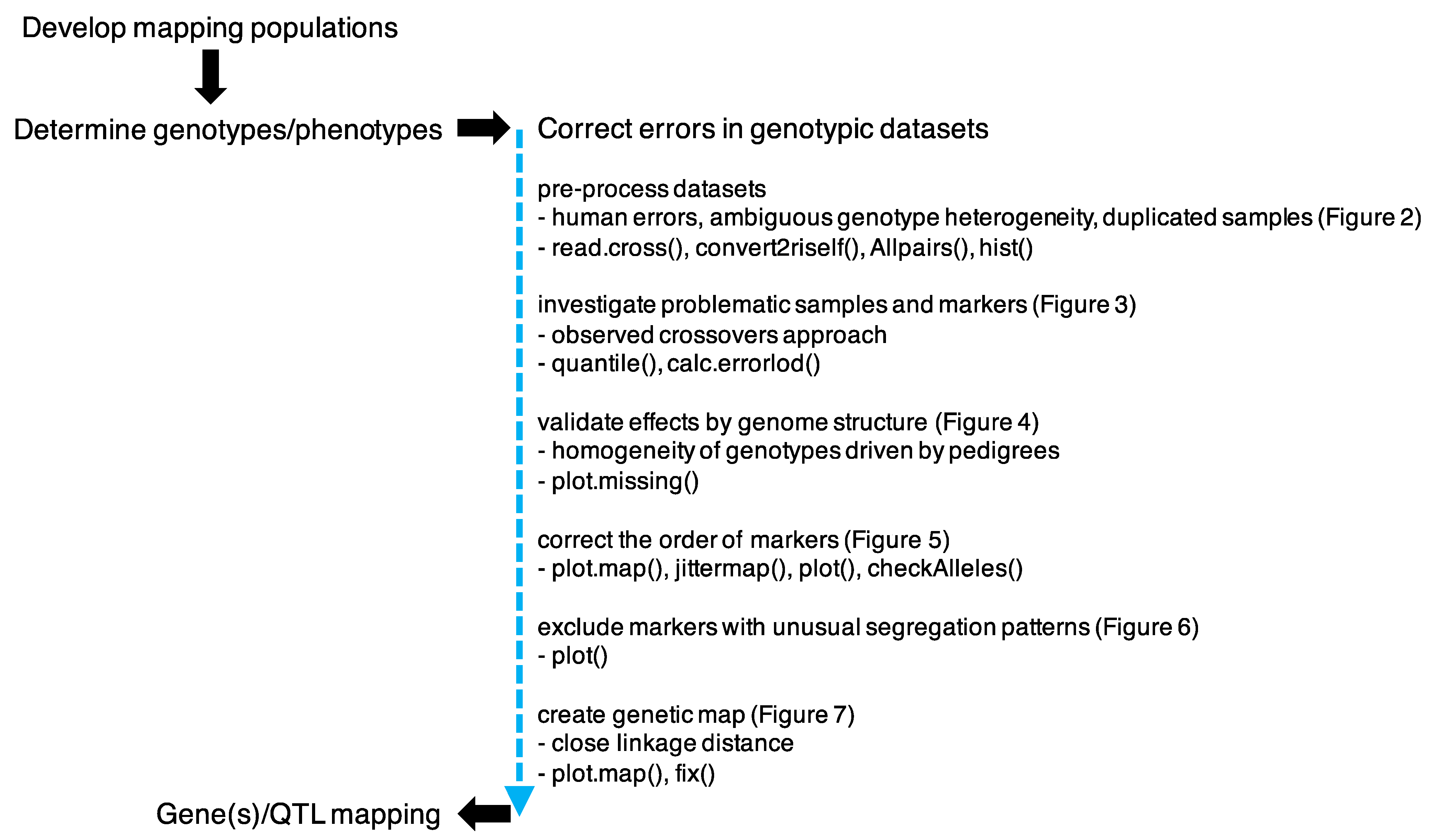
2.3. Genetic Map Development

We briefly describe the development of a genetic map here and detail this development in Section 3. To develop a genetic map, we used two different versions of the R environment (3.0.1 and 3.4.3) to implement the R/qtl package (V. 1.41-6, [3]). R/qtl processes diverse populations including F2, backcross (BC), and RIL populations. The Kosambi mapping function [13] and a genotyping error of 0.01% were used for linkage analysis. For general linkage grouping, a logarithm of odds (LOD) score of 3.0 and a recombination frequency (RF in the Kosambi function) of 0.372 were chosen as the significance criteria. Linkage map distance was estimated by maximum likelihood (ML) with the expectation–maximization (EM) algorithm [14]. The default maximum number of iterations and tolerance value were 1 × 10⁴ and 1 × 10⁻⁶, respectively.

3. Results and Discussion

Here, we present and discuss common steps to develop the genetic linkage map of a soybean RIL population. A workflow summarizing these steps is shown in Figure 1. Details of R codes are listed in Figure S1. Input files are included in Table S1 and Table S2.

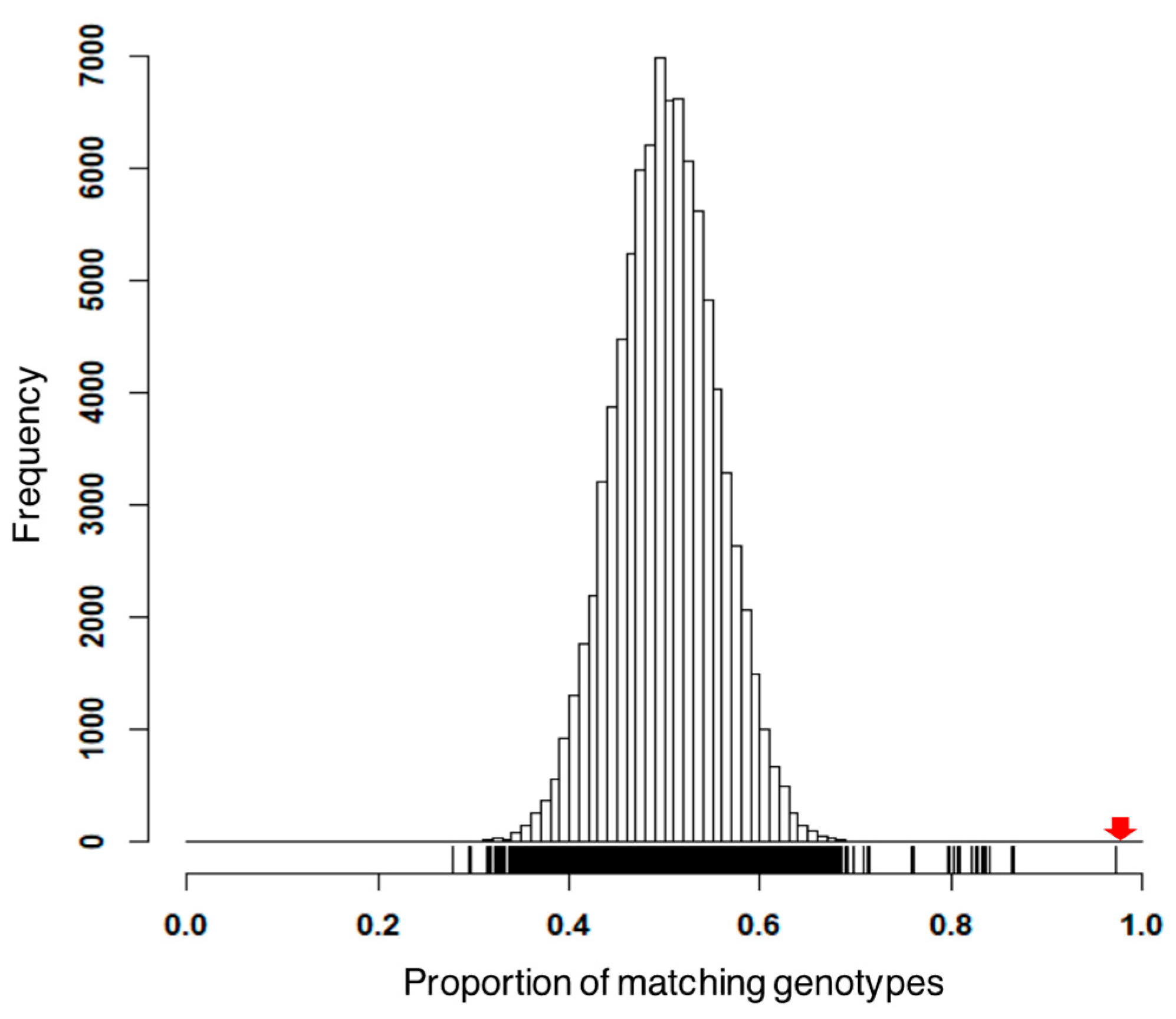
3.1. Preprocess Genotypic Datasets

Once the genotypic data are acquired, the first step is to convert ambiguous genotypes (e.g., ambiguous amplicons obtained from gel-based genotyping methods) to missing genotype codes (NA, N, or - symbols). Furthermore, heterozygous genotype codes (AB or H as determined by genotyping software packages) should be carefully considered as there is overall agreement that heterozygous genotypes are error prone unless such genotypes are validated using independent data such as high-depth whole genome sequencing (WGS) information. It is therefore considerable that heterozygous genotype calls be converted to missing genotypes when high levels of homozygosity are expected as a consequence of artificial selection.
We converted heterozygose calls to missing genotypes, since F6-derived soybean RILs were used in this study. After conversion, we used two R/qtl functions—specifically, read.cross() and convert2riself()—to process our RIL data. The first function emulates a typical BC data-type by reading RIL data and generating read-in data. The second function then converts the typical BC data-type to the RIL data type.
Next, we identified duplicate plant samples. Sample duplication could arise from human errors in advancing plant generations during population development steps (e.g., two seeds advanced from the same F6 plant in a RIL population) or the DNA extraction phase. Using the R/qtl function Allpairs(), we examined all possible pairs of individuals in the H × C population and calculated the degree of paired marker genotype identity. There were 44850 (300C2 = 300 × 299/2) possible pairings of the 300 individuals. The paired identity values for all pairs were displayed in a histogram according to their fractional degree of identity from zero identity (0.0) to complete identity (1.0) using the function hist() (Figure 2). Zero identity means the pair had a zero match of an A or B (e.g., H in F2) or NA (missing) genotype codes at all marker loci compared, whereas complete identity means the pair had a 100% match of genotype codes at every marker locus compared. The histogram peak value should theoretically be 0.5 in a RIL population (0.375 = 6/16 in the case of the F2 population).
The main challenge for the interpretation of paired marker genotype identity is to make a judgment call of what is a significant fraction of outliers (values that lie beyond the range of the far-right tail). Therefore, we should state a specified threshold for the fractional degree and display the R/qtl index number for members of the pair. From the perspective of inbreeding in population genetics, unlike a randomly mating population, selfing might be a common form of inbreeding, and each successive generation of selfing causes a theoretical 50% reduction in heterozygosity, while the allele frequencies in the population are unchanged. In our RIL population, the frequency of heterozygotes can be approximately 3% after five generations of selfing. Therefore, we chose 97% as a suitable threshold value. Our analysis showed that there were no outliers falling beyond the threshold value (Figure 2).

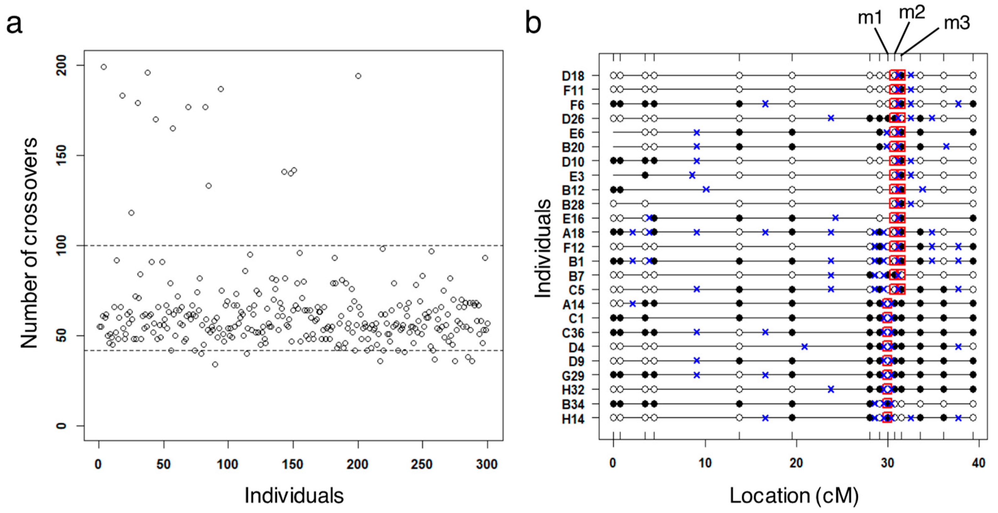
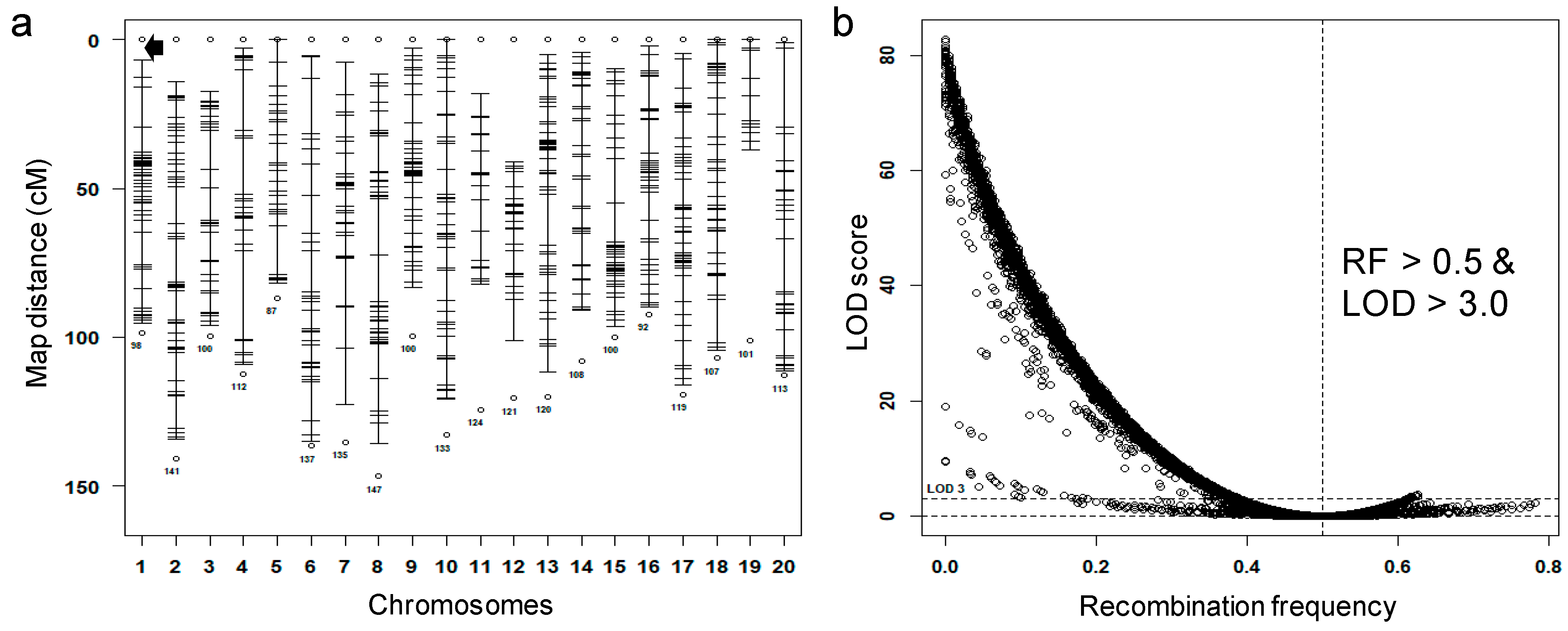
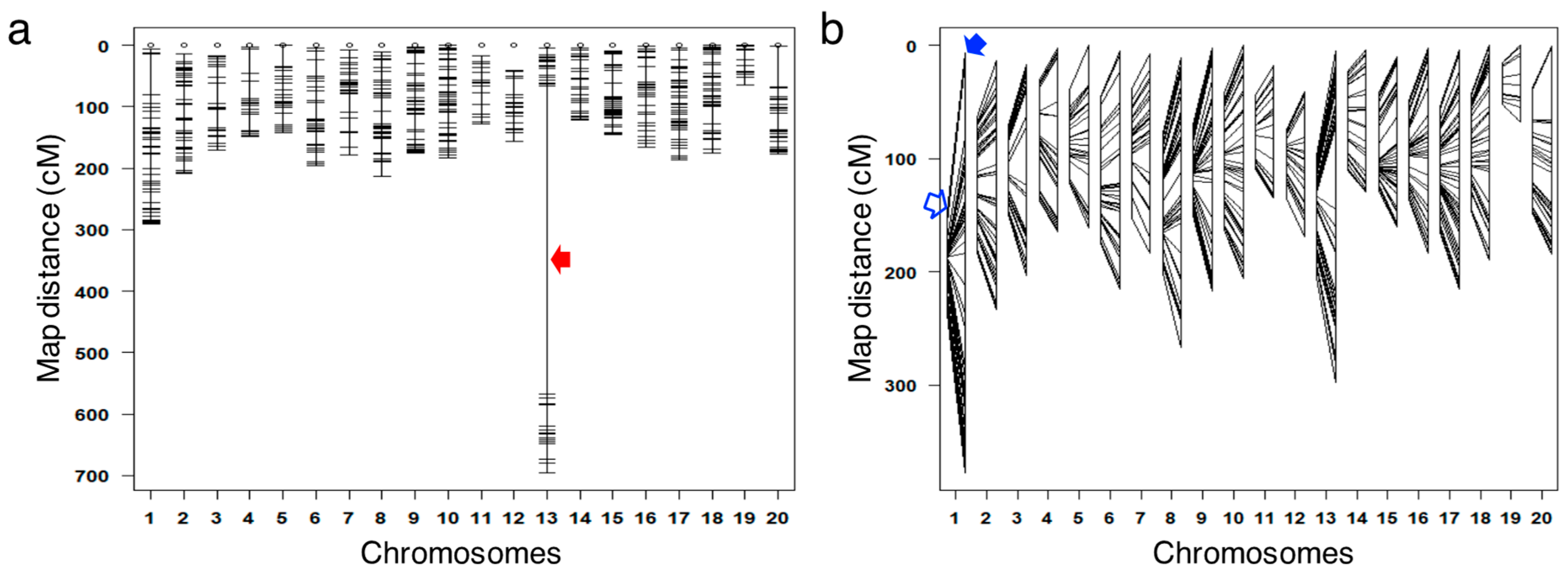
3.2. Identification of Potential False Crossovers

The occurrence of crossover events may vary by population size. According to the Beavis effect [15], a relatively small population size results in an overestimation of the QTL effect due to biased crossover. In this study, we used a large sample size (the number of RILs was 300) and constructed a genetic map with 751 polymorphic markers to avoid the bias due to crossover counts. In addition, we used codominant markers to access the recombinations driven by crossover. Notably, certain population types may be prone to biases between crossings; one example could be a BC population where large numbers of genome segments from a donor parent result in a large portion of monomorphic alleles by generation. Specifically, a BC population with a small population size is more likely to increase map distances with biased recombination information. Further, if outlying crossover counts (high or low) are observed in samples, such samples should be carefully assessed to determine whether they are the true members of the given population. Usually, samples with high or low crossover counts are not the descendants of parental mating in a population. Another possibility is sampling error, where poor DNA quality or sample mix-ups occur.
We plotted the number of crossovers in the RILs (Figure 3a). When the threshold value ranged from 42 to 100 (the parametric 5th and 95th percentiles of the value distribution identified using the R function quantile(); bottom and top horizontal bars, respectively), 15 RILs, which came from 5 F1 families (4, 4, 3, 2, and 2 from families A, B, C, D, and E, respectively), had crossover counts much greater than 100. Although setting the range of threshold values could be subjective, we decided not to retain the 15 RILs.
In cell division, double crossover or multi-crossover events within a narrow interval may occur with a minimum probability. In a linkage map with sparse map distances, if the genotype at a single marker position is out of phase relative to its flanking markers, e.g., a marker showing different polymorphism compared to two flanking markers within a narrow interval, it is very unlikely that a true double crossover event occurred. We calculated the LOD score of each marker with the null hypothesis that a genotype from an individual at each marker is correct using the function calc.errorlod(). The genotypic data of all other markers on the chromosome were considered by employing a hidden Markov model (HMM) [16]. To compute the stringent criterion, a LOD score ≥ 5 (a genotyping error rate of 1 per 10,000 or higher) was used to designate a genotype error. An example that shows a potential genotype error due to a false double crossover is shown in Figure 3b: 25 individuals with a LOD score ≥ 5 at three marker positions, BARC-011793-00875 (marker ID: m1), BARC-047428-12928 (m2), and Sat_134 (m3) (three markers positioned within 0.003 cM based on the soybean consensus map (the integrated genetic linkage map of soybean by Hyten et al. [11])). A total of 18 markers with a large LOD error were detected on chromosomes 2 (two markers), 5 (two), 9 (one), 14 (four), 15 (two), 17 (two), 18 (two), and 19 (three); further analyses excluded these markers.

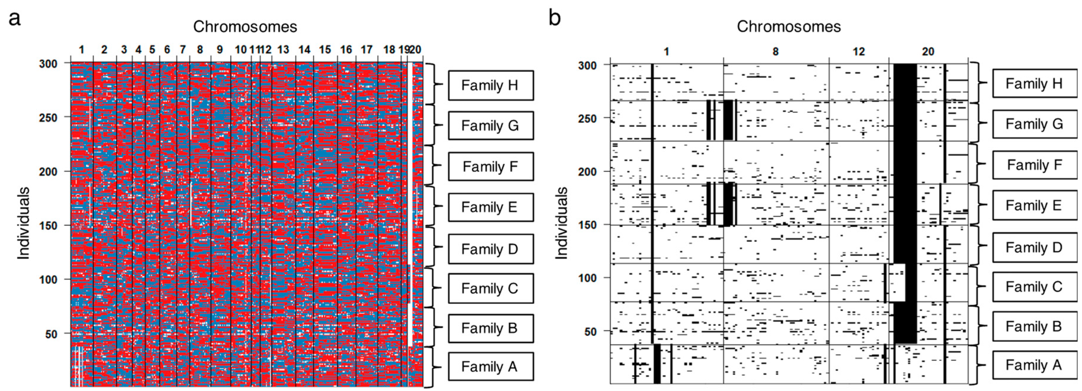
3.3. Validating Effects by Genome Structure

We then examined the homogeneity of genotypes driven by pedigrees in our population using the R/qtl function plot.missing() (Figure 4). On chromosomes 1, 8, 12, and 20, we observed several single families or multifamilies that possessed monomorphism for a given marker (Figure 4b). The loci on chromosome 20 in particular exhibited notable monomorphism across families. Family-specific monomorphism requires biological interpretation, such as gene conversion and natural variation of parents, since the observed monomorphism could be quite unusual. To retain potentially useful genetic information for those markers, we converted monomorphic codes to missing since such monomorphism would result in a false positive declaration of segregation distortion for those markers. To be justified in converting such genotypes to missing calls, it is advisable to test the segregation distortion of those markers (Section 3.5; no fluctuations in segregation ratios of family-specific monomorphic markers were observed) and switched alleles (Section 3.4; no switched alleles were detected) prior to the construction of the genetic map.

3.4. Correcting the Order of Markers

The use of consensus genetic linkage maps is powerful in developing a new genetic map because such maps provide a unified statistical framework for controlling for the effects of misplaced or incorrectly ordered markers or for saturated markers [11]. Given that our marker data type fits the framework of the soybean consensus map (all markers used in our study are present in the dataset used for the consensus map), we projected markers of our H × C population onto the consensus map to examine the relative marker positions and distribution of the population using the function plot.map() (Figure 5a). We then used the function jittermap() to generate slightly offset map positions by a 1 × 10⁻⁶ map distance to avoid regression failure in the QTL analysis functions in R/qtl. In cases where consensus maps or previous linkage studies are not available, studies using population-based genotyping data (e.g., a linkage test) can perform statistical tests to determine whether marker orders for each chromosome would be best for their own genetic map. Physical maps supported by reference genome assembly data may also be incorporated into resolving marker orders.
To correct marker loci with erroneously switched allele codes, we first evaluated the linkage between all possible pairs of markers using the recombination frequency (RF) and LOD. The RF was estimated by the RF between a pair of markers, and the LOD score for the RF was estimated by the test statistic of the null hypothesis that the RF is 0.5. Generally, the lower the RF value is, the higher the LOD score is, but if the A or B allele of one marker is switched in comparison with the B or A allele of another marker, then the RF value between the two markers may exceed 0.5 (up to a value of RF = 1.0). As a result, high RF values will cause high LOD scores. The relationship between the LOD score and RF was graphed using the function plot(), and we investigated whether any marker pairs had RF values greater than 0.5, which was coupled with a high LOD score (LOD > 3.0 using the R/qtl function checkAlleles()) (Figure 5b). A substantial number of marker pairs appeared to have RF values greater than 0.5 at an upward spike in the graph. No such markers, however, were flagged when a threshold LOD value (LOD = 3.0; 0.0002 as a p-value of the χ2 distribution) was applied. A more stringent threshold LOD value can also be applied (e.g., a LOD value of 7 after Bonferroni correction). An upward spike in a graph implies a switched allele condition, while a downward spike of RF values reflects linkage. Ideally, estimated RF values in the genotypic dataset would be 0.5 or less. Marker pairs with RF values greater than 0.5 may occur when imperfect allele segregation and/or missing genotypes in each of the unlinked markers are observed. Moreover, scatter in the curve will arise if marker genotypes are missing because RF values of 0.5 for given marker pairs can deviate from their true 0.5 value. A sampling error (an experimental error made by sample size) that originates from imperfect allele segregation in each marker may indeed arise in the range of 0.5 < RF < 0.6 when a large standard deviation is detected for RF (e.g., RF = 0.5 ± 0.2). In any case, small sample sizes will result in a large standard deviation for RF, and a large RF is also possible due to switched alleles for one member of the marker pair.

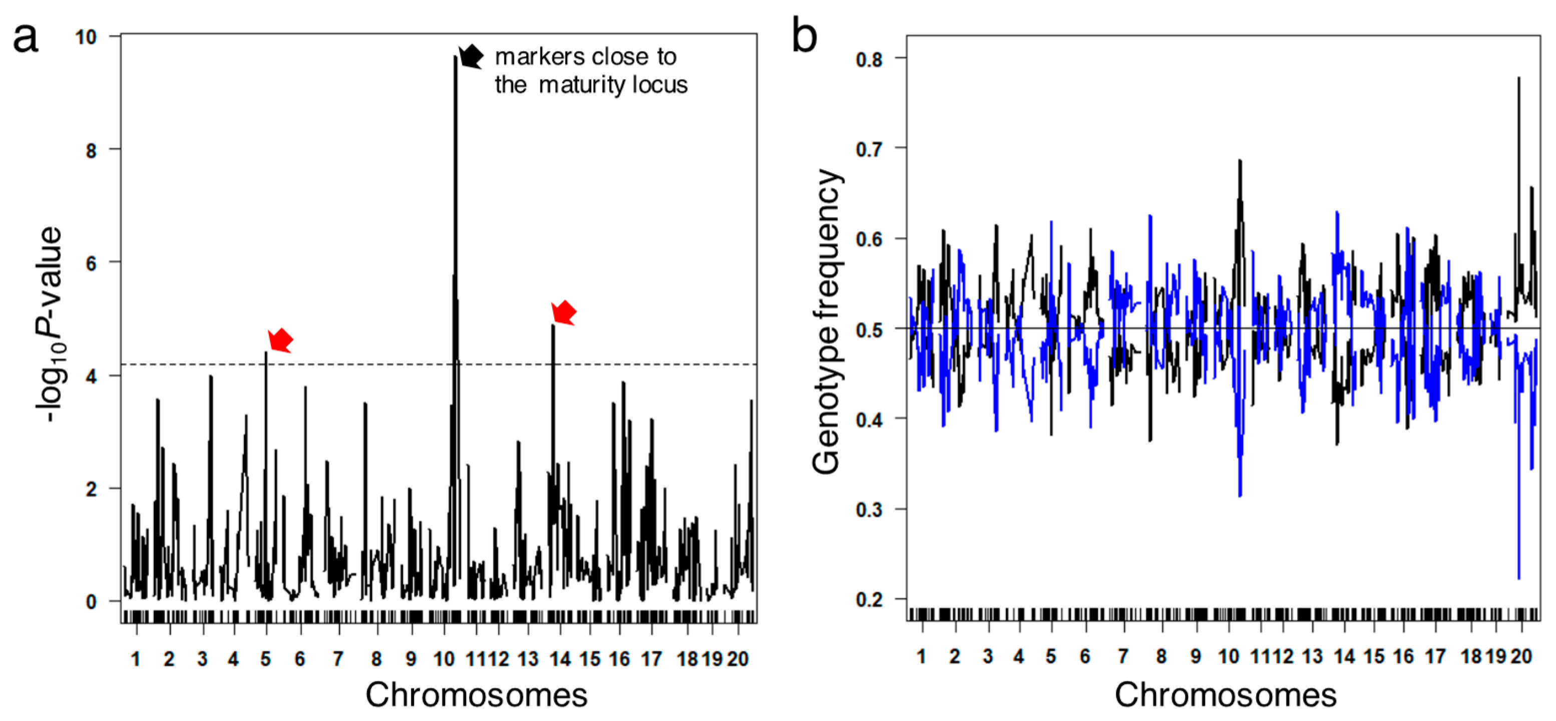
3.5. Segregation Analysis

We then looked at the segregation of each marker. χ2 tests were applied to determine whether each marker segregated with a ratio of 1 (AA):1 (BB) in the population. The outputted segregation data were ordered by chromosomes and markers using the function plot() (Figure 6a). A threshold value of 4.18 was obtained by -log10p-value, where the significance level (type I error rate) was set to 0.05 and Bonferroni correction was made (the total number of markers was 751). In the case of the LOD value, however, the value increases since the LOD value equals –log10(likelihood ratio test (LRT) value), where the LRT equals 0.2172 × p-value (the P-value from a χ2 distribution). For the LRT and LOD values, 1.446 × 10⁻⁵ and 4.8398 were obtained, respectively. If a marker has few genotypes for a χ2 test, Yates’ correction can be considered as an alternative. A total of nine markers in the H × C population showed fluctuations of segregation ratios on chromosomes 5, 10, and 14 (Figure 6a). Despite significant fluctuations in ratios, knowledge of genetic architecture can be exploited whether we retain specific alleles. According to the soybean consensus map, the soybean maturity allele [17] was positioned at 121.41 cM on chromosome 10, and the segregation distortion site included this allelic position. Therefore, the segregation distortion of six markers on chromosome 10 was likely due to inadvertent human selection of the C genotype (E2E2) for late maturity (vs. the H genotype e2e2 for early maturity). Therefore, we retained these six markers on chromosome 10 and dropped three markers on chromosomes 5 and 14 for the next step. After these markers were dropped, the RILs showed an overall genotype frequency of 1:1 across the whole genome (Figure 6b). Markers with distorted segregation could increase false positives in QTL analysis, especially in the simple interval mapping (SIM), and could be cofactors in both composite interval mapping (CIM) and multiple interval mapping (MIM) methods. Therefore, removing such markers requires careful consideration for specific crosses or plant species, because this influences the power for detecting true QTL.

3.6. Construction of the Genetic Map

After performing the above-mentioned steps, we created a draft genetic map for the H × C population using plot.map() (Figure 7a). To create a map, we translated an RF value between two adjacent markers into an intermarker distance using the Kosambi mapping function. Assuming that the marker order in the H × C population follows that of the soybean consensus map, we computed RF values between two markers on each chromosome in the population. Because of the exponential relationship between RF and the Kosambi map distance, when RF values increase to the limit of 0.5, the Kosambi map distance value explodes to infinity. Therefore, to correct undesirable gaps, we set the maximum RF value to 0.450, which equaled the Kosambi map distance of 73.61 cM. On chromosome 13, where a large gap appeared (a red arrow), we observed that the maximum distance of a gap was 500.8 cM, which was greater than 73.61 cM. Using the function fix(), we reduced the gap to 73.61 cM. One factor which should be considered critically when researchers apply this step to independent experiments is that larger map distances due to such gaps could overestimate R2 values and affect the estimation of confidence intervals for QTL [18,19].
Finally, we compared the final H × C map with the soybean consensus map V.4.0 (Figure 7b). The total map distance of the H × C map was 3769.4 cM, which was 1.6 times larger than that (2296.4 cM) of the soybean consensus map. The increased map distance in the H × C map compared to that in the consensus map could be attributable to a lower number of mapping populations incorporated in our mapping study. The average map distance of the H × C population was 5.21 cM.

4. Conclusions

Our study provides a workflow for cleaning genotypic datasets of plant populations in order to optimize subsequent genetic map development and mapping studies. The workflow is based on functions of the R/qtl package and a synthesis of R functions. A major advantage of this workflow is that users can use the workflow as a guideline to build a genetic map while requiring much less time and effort to prepare their own genotypic datasets. This is primarily because we have covered all important aspects which need to be considered when building the genetic map and can end up hidden in laboratories in an educational, concise way.
After performing the steps prior to those used to construct Figure 7, researchers can continue QTL/gene mapping studies of their target traits. For example, the R/qtl package provides two functions, scanone() for a single-QTL model (e.g., single marker analysis, interval mapping, selective genotyping by imputation analysis, and CIM) and scantwo() for a multiple-QTL model (e.g., MIM). Further, R/qtl provides diverse tools for QTL analysis using different strategies such as imputation analysis (selective genotyping) and composite or multiple interval mapping (good for setting up a criterion). Alternatively, input datasets could be prepared by using R/qtl when different software (ex. WinQTLCartographer [20], PLABQTL [21], or QTLNetwork [22]) are preferred.
The ultimate goal of genetic mapping is to identify the genetic variants that determine traits or phenotypes. Recent genomic study has been making significant progress in achieving genetic information, driving down genotyping costs and increasing capacity to acquire genotypes and genotype accuracy. Despite this progress, success in using such information to discover the association between genotypes and phenotypes will remain elusive unless phenotyping is further advanced to overcome current limitations in phenotype data collection in the plant species of interest.

Supplementary Materials

The following are available online at https://www.mdpi.com/2073-4395/9/4/196/s1, Figure S1: R codes, Table S1: Genotypic data, Table S2: Phenotypic data.

Author Contributions

Conceptualization, S.H. and T.G.L.; methodology, S.H. and T.G.L.; validation, T.G.L.; formal analysis, S.H.; investigation, S.H.; data curation, T.G.L.; writing—original draft preparation, S.H. and T.G.L.; writing—review and editing, T.G.L.; visualization, S.H. and T.G.L.; supervision, T.G.L.; project administration, T.G.L.

Conflicts of Interest

The authors declare no conflict of interest.

References

  1. Yu, J.; Buckler, E.S. Genetic association mapping and genome organization of maize. Curr. Opin. Biotechnol. 2006, 17, 155–160. [Google Scholar] [CrossRef] [PubMed]
  2. Yu, J.; Holland, J.B.; McMullen, M.D.; Buckler, E.S. Genetic design and statistical power of nested association mapping in maize. Genetics 2008, 178, 539–551. [Google Scholar] [CrossRef] [PubMed]
  3. Arends, D.; Prins, P.; Jansen, R.C.; Broman, K.W. R/qtl: High-throughput multiple QTL mapping. Bioinformatics 2010, 26, 2990–2992. [Google Scholar] [CrossRef] [PubMed]
  4. Broman, K.W.; Wu, H.; Sen, S.; Churchill, G.A. R/qtl: QTL mapping in experimental crosses. Bioinformatics 2003, 19, 889–890. [Google Scholar] [CrossRef] [PubMed] [Green Version]
  5. Broman, K.W.; Sen, S. A Guide to QTL Mapping with R/qtl; Springer: New York, NY, USA, 2009. [Google Scholar]
  6. Ihaka, R.; Gentleman, R.R. A language for data analysis and graphics. J. Comp. Graph. Stat. 1996, 5, 299–314. [Google Scholar]
  7. Weiss, M.G.; Stevenson, T.M. Registration of soybean varieties, V. Agron. J. 1955, 47, 541–543. [Google Scholar] [CrossRef]
  8. Johnson, H.W. Registration of soybean varieties, VI. Agron. J. 1958, 50, 690–691. [Google Scholar] [CrossRef]
  9. Fan, J.G.; Oliphant, A.; Shen, R.; Kermani, B.G.; Garcia, F.; Gunderson, K.L.; Hansen, M.; Steemers, F.; Butler, S.L.; Deloukas, P. Highly parallel SNP genotyping. Cold Spring Harb. Symp. Quant. Biol. 2003, 68, 69–78. [Google Scholar] [CrossRef] [PubMed]
  10. Akkaya, M.S.; Shoemaker, R.C.; Specht, J.E.; Bhagwat, A.A.; Cregan, P.B. Integration of simple sequence repeat DNA markers into a soybean linkage map. Crop Sci. 1995, 35, 1439–1445. [Google Scholar] [CrossRef]
  11. Hyten, D.L.; Choi, I.Y.; Song, Q.; Specht, J.E.; Carter, T.E.; Shoemaker, R.C.; Hwang, E.Y.; Matukumalli, L.K.; Cregan, P.B. A high density integrated genetic linkage map of soybean and the development of a 1536 universal soy linkage panel for quantitative trait locus mapping. Crop Sci. 2010, 50, 960–968. [Google Scholar] [CrossRef]
  12. Palmer, R.G.; Kilen, T.C. Quantitative Genetics. In Soybeans: Improvement, Production, and Uses, 2nd ed.; Wilcox, J.R., Ed.; American Society of Agronomy: Madison, WI, USA, 1987; Volume 5, pp. 135–209. [Google Scholar]
  13. Kosambi, D.D. The estimation of map distances from recombination values. Ann. Eugen. 1944, 12, 172–175. [Google Scholar] [CrossRef]
  14. Lander, E.S.; Green, P.; Abrahamson, J.; Barlow, A.; Daly, M.J.; Lincoln, S.E.; Newburg, L. Mapmaker: An interactive computer package for constructing primary genetic linkage maps of experimental and natural populations. Genomics 1987, 1, 174–181. [Google Scholar] [CrossRef]
  15. Xu, S. Theoretical basis of the Beavis effect. Genetics 2003, 165, 2259–2268. [Google Scholar] [PubMed]
  16. Eddy, S.R. What is a hidden Markov model? Nat. Biotechnol. 2004, 22, 1315–1316. [Google Scholar] [CrossRef] [PubMed] [Green Version]
  17. Bernard, R.L. Two major genes for time of flowering and maturity in soybeans. Crop Sci. 1971, 11, 242–244. [Google Scholar] [CrossRef]
  18. Darvasi, A.; Weinreb, A.; Minke, V.; Weller, J.I.; Soller, M. Detecting marker-QTL linkage and estimating QTL gene effect and map location using a saturated genetic map. Genetics 1993, 134, 943–951. [Google Scholar] [PubMed]
  19. Darvasi, A.; Soller, M. A simple method to calculate resolving power and confidence interval of QTL map location. Behav. Genet. 1997, 27, 125–132. [Google Scholar] [CrossRef] [PubMed]
  20. Wang, S.; Basten, C.J.; Zeng, Z.B. Windows QTL Cartographer 2.51; Department of Statistics, North Carolina State University: Raleigh, NC, USA, 2010. [Google Scholar]
  21. Utz, H.F.; Melchinger, A.E. PLABQTL: A program for composite interval mapping of QTL. J. Quant. Trait Loci. 1996, 2, 1–5. [Google Scholar]
  22. Yang, J.; Hu, C.; Hu, H.; Yu, R.; Xia, Z.; Ye, X.; Zhu, J. QTLNetwork: Mapping and visualizing genetic architecture of complex traits in experimental populations. Bioinformatics 2008, 24, 721–723. [Google Scholar] [CrossRef] [PubMed]
Figure 1. Correction of pervasive errors in genotypic datasets in the development of genetic maps. Common steps to develop genetic maps are presented (the left column). The key steps in correcting pervasive errors in genotypic datasets are presented (the right column) in the order in which they are performed in this article. Specific named R/qtl and R functions are immediately followed by single closed brackets.
Agronomy 09 00196 g001
Figure 2. Identification of duplicated individuals. Histogram of the proportion of markers for which pairs of individuals have matching genotypes. The top portion of the histogram (a degree of 0.5) represents an idealized distribution of the frequency of matching genotypes in a recombinant inbred line (RIL) plant population. The fraction was computed for two-way comparisons of all markers, which ranged between 0.0 (0% identical) and 1.0 (100% identical). The majority of individuals in this population showed between 30% and 70% of genotypes shared. A fractional degree, 0.97, is marked by a red arrow on rug lines and used as a threshold value to indicate duplicate individuals.
Agronomy 09 00196 g002
Figure 3. Identification of problematic individuals and markers based on crossovers. (a) Numbers of observed crossovers in each individual line are displayed. Threshold values of 100 crossovers (the parametric 95th percentile of the value distribution; top horizontal bar) or less are accepted as the criteria for assigning the number of crossovers to each individual, resulting in 15 individuals identified as outliers. The bottom horizontal bar indicates the parametric 5th percentiles of the value distribution; (b) genotypes that show potential false crossovers on chromosome 19. Red-colored quadrangles flag markers with a high logarithm of odds (LOD) score, indicating the presence of potential genotypic errors. The genetic map distance between adjacent markers is 0.003 (between markers m1 and m2) and 0.001 cM (m2 and m3) based on the consensus map. Those three markers were excluded, since they were most likely caused by genotyping errors. Empty and black-filled circles indicate ‘C’ and ‘H’ genotypes in the population as described in the Materials and Methods. The crossover event is marked by a blue cross.
Agronomy 09 00196 g003
Figure 4. Family-specific monomorphism was detected in the population. (a) Polymorphic markers are color-coded (blue: Harosoy genotype, red: Clark genotype, white: mono-allelic and missing genotypes). Each of the distinguishable groups (eight family groups (A through H) in the population) is displayed by group designation on the right. The y-axis represents the number of individual plants. The values of 1–20 at the top of the figure indicate the 20 chromosomes of soybean; (b) high-density mono-allelic genotypes specific to a few families are indicated by black cells on chromosomes 1, 8, 12, and 20.
Agronomy 09 00196 g004
Figure 5. Determination of genotypes that occurred in erroneous order. (a) Marker positions (both marker order and map distance) within chromosomes are projected based on the consensus map. Empty dots represent the beginnings and ends of chromosomes. The length (cM; centimorgan) of each chromosome is labeled under the chromosome. The gap marked by a black arrow is the genetic map distance between the first marker located at 0.00 cM and the next marker; (b) a plot of the logarithm of odds (LOD) scores against the estimated recombination frequency (RF) for all marker pairs indicating erroneous markers. The threshold values (RF >0.5 and LOD >3.0) were shaded in gray.
Agronomy 09 00196 g005
Figure 6. Unusual segregation patterns of genotypes. (a) Major fluctuations in segregation ratios in genotypic datasets of the H × C population were detected (red arrows on chromosomes 5 and 14 and black arrow on chromosome 10). We retained the markers (near the black arrow) on chromosome 10, since such fluctuations were likely due to the artificial selection. A threshold value of 4.18 (horizontal bar) for the segregation ratio was determined by calculating a P-value using a χ2 test (alpha level = 0.05) and then applying the Bonferroni correction. Some picks represent multiple data values within the narrow chromosome interval; (b) after the removal of fluctuating genotypes (red arrows in Figure 6a), a mirror image (black color for the ‘C’ genotype in the H × C population; blue for ‘H’) was observed across chromosomes, which verified the 1:1 genotype frequency for each marker.
Agronomy 09 00196 g006
Figure 7. A genetic map was developed using corrected genotypic data. (a) The draft genetic map was developed using the H × C population (termed the H × C map). Unlike in Figure 5a, which was developed based on the map distance of the consensus map, the map distance in the H × C map was drawn based on the H × C population. Marker orders were based on the consensus map. A gap (red arrow) that spans approximately 500 cM on chromosome 13 was observed; (b) the final H × C map (marked by a filled blue arrow on chromosome 1; representative of all 20 chromosomes) was compared to the consensus map (open blue). Markers mapped to two different maps are connected by black lines. The corrected genetic linkage on chromosome 13 was used in the final H × C map.
Agronomy 09 00196 g007

