Article

Szarvasi-1 and Its Potential to Become a Substitute for Maize Which Is Grown for the Purposes of Biogas Plants in the Czech Republic

Department of Agroecosystems, Faculty of Agriculture, University of South Bohemia in České Budějovice, Branišovská 1457, 370 05 České Budějovice, Czech Republic
*
Author to whom correspondence should be addressed.
Agronomy 2019, 9(2), 98; https://doi.org/10.3390/agronomy9020098
Submission received: 21 January 2019 / Revised: 11 February 2019 / Accepted: 17 February 2019 / Published: 19 February 2019
(This article belongs to the Special Issue Forage and Bioenergy Crops)

Abstract

:
The domestic biogas market has been developing rapidly, and legislation (The Act) supporting the use of renewable energy sources has come into force. In light of this act and investment support from national programs co-financed by the European Union (EU), the total number of biogas plants has recently increased from a few to 600. The total capacity of electricity generation of those 600 installed plants exceeds 360 Megawatts (MW) (as of mid-2018). Such dynamic growth is expected to continue, and the targets of the National Renewable Energy Action Plan are projected to be met. The use of waste material, which was urgently needed, was the original aim of biogas plants. However, in certain cases, the original purpose has transformed, and phytomass is very often derived from purpose-grown energy crops. Maize is the most common and widely grown energy crop in the Czech Republic. Nevertheless, maize production raises several environmental issues. One way to potentially reduce maize’s harmful effects is to replace it with other suitable crops. Perennial energy crops, for example, are possible alternatives to maize. A newly introduced species for the conditions of the Czech Republic, Elymus elongatus subsp. ponticus cv. Szarvasi-1, and some other well-known species—Phalaris arundinacea L. and Miscanthus × giganteus—are suitable for Czech Republic climate conditions. This paper presents the findings of the research and evaluation of environmental, energy-related, and economic aspects of growing these crops for use in biogas plants. These findings are based on 5-year small-plot field trials. The energy-related aspects of producing Elymus elongatus subsp. ponticus cv. Szarvasi-1, Phalaris arundinacea L., and Miscanthus x giganteus are reported on the basis of experiments that included measuring the real methane yield from a production unit. The economic analysis is based on a model of every single growing and technological operation and costs. The environmental burden of the individual growing methods was assessed with a simplified life cycle assessment (LCA) using the impact category of Climate Change and the SimaPro 8.5.2.0 software tool, including an integrated method called ReCiPe. The research findings show that Szarvasi-1 produces 5.7–6.7 Euros (EUR) per Gigajoule (GJ) of energy, depending on the growing technology used. Szarvasi-1 generates an average energy profit of 101.4 GJ ha−1, which is half of that produced by maize (214.1 GJ ha−1). The environmental burden per energy unit of maize amounts to 16 kg of carbon dioxide eq GJ−1 compared with the environmental burden per energy unit of Szarvasi-1, which amounts to 7.2–15.6 kg of CO2 eq GJ−1, depending on the yield rate. On the basis of the above-mentioned yield rate of Szarvasi-1, it cannot be definitively recommended for the purpose of biogas plants in the Czech Republic.

1. Introduction

Central Europe and the Czech Republic are characterized by intensive farming, and there has been an overproduction of produced commodities (raw materials and foodstuffs), as well as problems with their sale. Energy generated from biogas shows that this industry has the potential to stabilize the farming sector. Biogas can be made from agricultural products, waste, or animal excrements [1]. The term “biogas” means a mixture of gases generated by the anaerobic fermentation of wet organic matter carried out with equipment (reactor, digester, etc.) called a biogas plant (BGP) [2]. Considering the current conditions in the Czech Republic, biogas is used mostly for the combined generation of energy in so-called co-generation units with a reciprocating combustion engine. The year-long use of biogas stations requires a continuous supply of organic matter to the fermenter. Therefore, input plant material has to be conserved (ensiled). Forage crops (Dactylis glomerata, Arrhenatherum elatius, Phalaris arundinacea, etc.) are frequently used as input material [3]. Mužík and Kára [4] stated that most of the plant material used for the generation of biogas is produced by agriculture. Farm animal excrement, side products of crop production, and energy crops are especially common. Species originating the input material (e.g., maize, grass, or manure) have turned out to be the decisive factors determining the impacts of a biogas unit on the environment [5,6]. Plant biomass represents more than 50% of all biogas substrates. Maize silage and other types of phytomass (made mostly from perennial grass) represent up to 80% of the plant biomass. Converted to energy content, plant phytomass input represents up to 80% of the energy content of all substrates [7]. Grasslands have become more significant for the generation of energy. Fallow grasslands can be used for the production of energy crops, and perennial grasslands produce sufficient phytomass. They are considered a very promising solution. As this research shows, there are two possibilities for phytomass use: burning dry phytomass or processing wet phytomass by anaerobic digestion to produce biogas [8].
The number of biogas stations has recently increased considerably in the Czech Republic. The original intent was to use organic waste material in these stations; however, the phytomass of energy crops is mostly used as the primary raw material. Maize is the most frequently used energy crop in the Czech Republic. The production of maize contributes heavily to anthropogenic emissions and poses many environmental problems. Replacing maize with other energy crops has shown promise for reducing environmental impacts. Perennial energy crops are considered good alternatives to maize. Miscanthus × giganteus (hereinafter referred to as “M × G“), Reed Canary Grass (Phalaris arundinacea L.) (hereinafter referred to as “RCG”), and Elymus elongatus subsp. ponticus cv. Szarvasi-1 (hereinafter referred to as “Sz-1”) are three such crops. The last is a new species introduced to the Czech Republic. Biemans et al. [9] emphasized that the large-scale introduction of regionally unknown energy crops requires knowledge of their environmental impacts. Dauber et al. [10] asserted that not only the energy-related and economic aspects, but also the environmental aspects of growing energy crops must be considered. In order to consider the environmental aspects of energy crops, analyses such as a life cycle assessment (LCA) can be employed [11,12]. This paper′s objective is to summarize the findings for Elymus elongatus subsp. Ponticus cv. Szarvasi-1, a new energy crop in the Czech Republic, and to consider possibilities for its use on the basis of its environmental, energy-related, and economic aspects.

2. Materials and Methods

2.1. The Life Cycle Assessment Part of The Study

2.1.1. Goal and Scope Definition

The goals of this study are to quantify the environmental burden of the growing cycles of particular energy crops to determine their energy efficiency and to evaluate the economic aspects of growing energy crops. The results of this research may be used to motivate environment-friendly farming systems and as a source of information for agricultural subjects that focus on phytomass and its energetic use. Four crops were analyzed and evaluated, in accordance with LCA norms, to quantify their environmental impacts and to identify the key environmental process. All four crops are considered suitable for biogas processing [13,14].

System Boundaries

This paper describes a technological process for growing energy crops. This process has been set up on the basis of primary (field trials carried out on the University of South Bohemia’s land in České Budějovice) and secondary data (the secondary data are from a database called Ecoinvent v3 [15], reference books, and the technical and technological norms for agricultural production). The Ecoinvent v3 database includes data from Central Europe. Primary data were gathered from 2013 to 2017, and secondary data were gathered from 2000 to 2018. The intensity of fertilization and agrotechnological methods were established according to ordinary intensive agricultural technologies [16,17,18,19,20,21,22,23,24,25]. Technologies for Sz-1 and RCG were also set up, too. Agrotechnological operations were also incorporated into the model system: from pre-seeding preparation, through harvesting the main product, to the transport of farming machinery, as well as the number of seeds used, the production and use of crop-protecting agents, the production and use of fertilizers, and the harvest and transport of the main product from the harvest site. Infrastructure processes and waste management were excluded from this research. As far as this research and paper are concerned, the transport distance from the factory to the field did not exceed 10 km.

Functional Unit

A functional unit related to a production unit and an area unit was chosen for the purpose of this research. The production unit is expressed as 1 GJ of energy generated by the electrical energy produced from the biogas produced by the anaerobic fermentation process in a co-generation unit; the area unit is expressed as 1 ha of a monoculture of the selected energy crops. The environmental impacts of the processes being researched were not divided into two or more processes (all of the upper plant material was considered the final product in this research), and there were no allocation methods employed.

Sources of Inventory Data

Field trials with the selected energy crops were established for this research. The trials were sources of primary data for LCA and the assessment of energy-related and economic aspects when the life cycle was studied. The station’s characteristics are described in following Table 1 and Table 2.

Investigated Crops

(1) Szarvasi-1 and Reed Canary Grass
Reference stands of the investigated grass species (RCG and Sz-1) were established in accordance with growing technologies (System boundaries). The existing perennial grasses were removed with glyphosate before the reference crops were established. The soil was loosened with a mid-deep plow to 14–18 cm depth and leveled with a cultivator within the framework of pre-seeding preparatory works. Mulch was put onto the land, which was treated with glyphosate in August 2013 before autumnal seeding. Mineral fertilizers were added to the soil before seeding, one year before the crop stand was established. The initial dose of mineral fertilizer per plot (125 × 800 cm) was 300 g of triple superphosphate (hereinafter referred to as SF3), 200 g of ammonium sulphate (hereinafter referred to as AS), 100 g of ammonium nitrate (hereinafter referred to as AN), and 625 g of potassium salt (hereinafter referred to as PS). The initial dose was identical for all plots (Table 3). The fertilizer doses were adjusted according to the purpose of use of every single crop stand. However, doses of fertilizers were different in the productive years (Table 4). For grasslands cultivated for the purpose of BGP, fertilizer was applied in two phases between two dates of mow. The mineral fertilizers AS, PS, and SF3 were applied in spring, before the growing season started, and AN was applied just after the first date of mow. Seeding was carried out on 30 August 2013 using a seeding machine to ensure seeding was accurate and precise. The seeding rate was 5 g of seeds per 1 m2 for RCG and 2.5 g of seeds per 1 m2 for Sz-1 (mean germinability of RCG = 39% and mean germinability of Sz-1 = 89% [27]). All plots were rolled after seeding.
(2) Miscanthus × Giganteus
The M × G stands were established using accepted practices (section “System Boundaries”). The density of planted rhizomes was 0.5 m × 1 m (Table 5). Mid-deep plowing to 14–18 cm depth was carried out in autumn 2012 (40 tons of manure per hectare were plowed into the soil). Pre-seeding preparatory works were carried out with a cultivator, and the soil was leveled in the spring. Crops were seeded and the soil was rolled and leveled. The newly emerged crop stand of Miscanthus × giganteus was treated with herbicide in order to protect it from dicotyledonous weeds. Weed control was applied once more during the growing season. This consisted of mechanical inter-row treatment. It is highly recommended to keep M × G crop stands free of weeds in the first year of establishment [25]. Doses of fertilizers were adjusted according to the purpose of use of every single crop stand. For the crop stand grown for the purpose of BGP, fertilizers were applied in two phases between two dates of mow. The intensity of maize fertilization is shown in Table 6.
(3) Maize (as a Reference Crop)
Maize reference crop stands were established each spring starting in 2013. Buckwheat, spring barley, or oat was the previous crop. The potential influence of previous crops was not taken into account in this study. The plot was prepared before seeding: 20 tons of manure per hectare was applied in autumn and plowed into the soil (mid-deep plow). The plot was leveled with a cultivator within the framework of pre-seeding preparatory works. Seeding was performed with a sowing machine for accuracy and precision. The seeding rate was 30 kg of seeds per hectare. A silage herbicide was applied to the plot. SF3 mineral fertilizer was applied in a dose of 200 kg per hectare during the sowing itself; urea (hereinafter referred to as U) was also applied in a dose of 200 kg per hectare (46% of N); PS was also applied in a dose of 104 kg per hectare. The density of the crop stands was 75 × 13 cm, and seeds were 5 cm deep in the ground. The crop stand was treated chemically with herbicide during the growing season to protect it from dicotyledonous weeds. Another dose of nitrogen was supplied (125 kg of U per hectare) at the phase of the fifth or sixth leaf. The intensity of maize fertilization is shown in Table 7.

Harvest

The interval between dates of mow (and harvest dates) and the dates of mowing were adjusted according to the purpose of use of the phytomass (previous parts of the methodology). Perennial energy crop stands (Sz-1, RCG, and M × G) grown for the purpose of BGP were always mowed and harvested two times per year when dry matter content was 28–38%. Maize crop stands were always harvested once (in September), and the harvest depended on dry matter content (the optimal percentage is 28–35%).

Software Data Inventorization

The cradle-to-gate principle, which is based on calculating the life cycle of a product from material supply to the end of the production (growing) process, was selected for the purpose of this research. The phases of use and removal of the product were not included in this study. Inventorization data from the Ecoinvent database [28] and SimaPro 8.5.2.0 program were used in this study (Table 8). These data were modified and enriched with data gathered from field trials and reference books (Section 2.1.1). SimaPro 8.5.2.0 software with an integrated database called Ecoinvent v3 [28] was used to develop models of the production systems. The inventoried data and details of the collection of the data are described in Section 2.1.1.

2.1.2. Life Cycle Impact Assessment

A simplified life cycle assessment method is an instrument for emission load calculations and is defined by specific norms [13,14]. The results of this research are related to the impact category of climate change, which is expressed in carbon dioxide equivalents.
SimaPro 8.5.2.0 software and ReCiPe Midpoint (H) V1.13/Europe Recipe H., an integrated method, were used for emission load calculations. One GJ of final product (dry matter) energy and an area unit (1 ha) were used as functional units. The technological processes of growing the selected crops were set up on the basis of primary data (field trials carried out on plots at the University of South Bohemia) and secondary data (data gained from the Ecoinvent v3 database, reference books, and technical and technological norms for agricultural production—see System boundaries). Data related to Central Europe were determined from the database. Primary data were collected from 2013 to 2017 and secondary data were collected from 2000 to 2017. The intensity of fertilization and agrotechnological methods were determined on the basis of typical intensive farming technologies. All of the agrotechnological operations—from pre-seeding preparatory works to the number of planted seeds, production and application of herbicides, production and application of fertilizers, transport of agricultural machinery, harvest and transport of the main products—were incorporated into the model system. The calculated emissions included not only those produced by the above-mentioned processes but also field emissions produced (especially dinitrogen monoxide ones). Emissions are mostly caused by nitrogenous fertilizers (farm or industrial ones) [29,30]. The Intergovernmental Panel on Climate Change (IPCC) methodology was used to calculate the quantity of emissions [31,32,33].
The results of the five-year growth of maize, RCG, Sz-1, and M × G for energy-generating purposes are summarized in this paper. According to the methodology applied and data gathered during the study period (dry matter yield rate, inputs and outputs of cycle of growth), the life cycles (from pre-seeding soil preparation to harvest, transport, and silage of the harvested material) of the above-mentioned crops were determined, and the environmental impacts were calculated. As mentioned above, the results of this research are related to the impact category of “climate change”, which is expressed in carbon dioxide equivalents (CO2 eq = 1 × CO2; 2 × CH4; 298 × N2O). The metric is based on the efficiencies of greenhouse gases [34,35]. The potential impact of N2O and CH4 emissions (they are produced by crops grown on arable land) on global warming (one-hundred-year interval) is 298 times and 23 times higher than the potential impact of carbon dioxide [36].

Determination of Field Emissions

The application of mineral and organic nitrogenous fertilizers results in the release of so-called direct and indirect emissions of dinitrogen monoxide (expressed as carbon dioxide equivalents). The emission load was determined in accordance with the IPCC methodology called Tier 1 [31] and the Czech national report on the inventory made of greenhouse gases (the agricultural section) [37].

2.2. Biogas Efficiency Determination

Biogas (or methane) efficiency was determined in this study. On the basis of the resulting values, the suitability of each energy crop for BGP purposes was determined.
A tested substrate was incubated in BGP fermenter digestate. It did not show any abnormalities, such as acids, pH, etc. A mixed digestate of fermenters from various BGPs was used, with various “nutrition” sources for bacteria: maize, grass, beef slurry, etc. All BGPs using residual substrates, pork slurry, bird excrement, etc. were excluded from the digestate. The digestate was filtered before use with a 2-mm sieve and then incubated at 40 °C for one week. Homogenized substrate was added to it, and it was incubated in anaerobic conditions at 40 °C. Gas was caught in a flask with a scale and the quantity was determined. Entering this flask was gas bubbling through a solution of NaOH, and carbon dioxide was captured while CH4 was produced. There was a negligible error caused by minor gases that were not captured in the hydroxide. The quantity of such gas was up to 2%. The incubation lasted until the substrate’s potential was exhausted, and the inoculum was used as a blind sample. The quantity of gas generated during this blinded test was deducted from the results for the substrate. There was measurement uncertainty expressed as the extended uncertainty with a coefficient of expansion of k = 2 (significance level of 95%). The above-mentioned uncertainty did not apply to any values below the limit of quantification.

2.3. Economic Efficiency

The economic analysis was based on models of all growing and technological operations and costs. This analysis included an economic assessment of the variable and fixed costs of machinery, the total costs of 1 ha, yield of the main product, costs of a unit of the main product (1 GJ of generated energy), and profit in the case of market production and use in both directions. The technical and technological norms for agricultural production and input data on growing perennial crops in practice were used as sources of information and examples.
The costs of growth include all the costs associated with growing energy crops. The costs of establishment, fertilization, harvest, field and road transport, weed control, and overhead costs are considered the main costs. Most of the expenses include the cost of work and machinery equipment.

3. Results and Discussion

3.1. Phytomass Yield and Potential Profit

Dry matter yield is presumed to be the primary figure of the total assessment. As expected, maize produced the highest average yield of phytomass (or dry matter) (14.4 tons of dry matter per hectare, on average). It produced a relatively stable yield in a short period of time compared with perennial crops. Table 9 shows the summary results achieved during the first four years of crop growth. Perennial crops produced <1/2 of the overall dry matter yield of maize during these four years. M × G was the highest-yielding perennial crop (9.6 tons of dry matter per hectare, on average). From this perspective, the period for which perennial crops and maize were compared is untimely, as perennial crops usually achieve their yield potential three years after the crop stand is established [22,26]. The yield potential is as follows: 12 tons of dry matter per hectare for RCG [24,38], 15–25 tons of dry matter per hectare for M × G [16,39,40,41,42], and <15 tons of dry matter per hectare for Sz-1 [22,43]. The fact that C4 crops (maize and M × G) are considered more efficient energy crops than C3 grasses (RCG and Sz-1) has to be taken into account; C4 crops have higher photosynthetic rates [16]. The fact that the perennial crop stands were not harvested in the first year (compared with maize) was also considered. However, when evaluating the environmental burden during our four-year cycle, the first year must also be included in this evaluation (because of energetic inputs).
Yield of phytomass, harvest time [44], and silage capacity [45,46] play crucial roles in the overall yield of methane [47,48]. To test the specific efficiency of CH4—the amount of methane produced by 1 kg of dry matter (m3 CH4 kg−1 of dry matter)—the values were calculated. Depending on the yield in the first four years, maize can produce three-fold higher amounts of methane (or energy in GJ per hectare) than perennial crops. Statistical assessment (Least Significant Difference—LSD test) and variance analysis (ANOVA) are shown in Table 10 and Table 11, which show that yield is influenced by the intensity of treatment and energy-related parameters (p ≤ 0.05) by species (Table 10). Analysis of variance (ANOVA) shows that energy efficiency is statistically significant (p ≤ 0.001) and influenced by species (more than 63%) (Table 11).
Crops were harvested in accordance with the methodology and on the dates shown in Table 12; the dry matter content at the time of harvest was recorded (Table 13). There are many recommendations for fixing the date of mow; nevertheless, the date of harvest is not crucial for the overall efficiency of methane [43]. For example, Mast et al. [49] recommended fixing the date of the second mow of Sz-1 to at least the beginning of October.
Perennial grass yields were higher in the initial years; this finding is confirmed by the statistical assessment (p ≤ 0.05) (LSD test) (Table 14). Therefore, it is possible to determine the optimal date of Sz-1 harvest for the purpose of BGP according to lignocellulose content. Alaru et al. [50] stated that Sz-1 contains an average of 38% cellulose, an average of 27% hemicellulose, and an average of 10% lignin. Miscanthus (Sacchariflorus) contains 42% cellulose, 30% hemicellulose, and 7% lignin. Hemicellulose is hydrolyzed more easily and produces more methane and less tar than cellulose. Both are more biodegradable than lignin. The total methane efficiency depends on the lignin content: every 1% of lignin in the biomass decreases the methane efficiency by 7.49 L of CH4 kg−1 (on average) [50].
There were no significant differences in methane efficiency [CH4 (l kg−1 of dry matter)] between the dates of mow [49,51]. However, methane efficiency depends greatly on the lignin content. So, methane efficiency increases if the date of harvest is postponed. The dates of mowing were fixed in this study. Hemicellulose, cellulose, and lignin are the three main elements of biomass and they usually represent 20–40%, 40–60%, and 10–25% of lignocellulose biomass [52]. Cellulose is the most common organic compound on Earth; biomass cell walls are mostly made of it, and it typically represents 33% of plant biomass [50]. However, there is a lack of information on the optimal Sz-1 harvest date for the purpose of BGP [49].
Table 13 shows the average content of dry matter (%) in the phytomass at harvest, and it plays a crucial role in the silage process and biogas (or methane) efficiency. For perennial crops, the average content of dry matter was higher at the time of the second mowing [49]. In most cases, there is high-quality silage and the highest efficiency of biogas if dry matter represents from 28% to 35% of the biomass [51,53]. A low content of dry matter worsens the silage quality and lowers the water leakage and biogas efficiency [54]. On the other hand, if the optimal level of dry matter content is exceeded, it becomes less degradable, less storable, and of lower quality [53]. Qualitative and quantitative parameters of phytomass (or silage) determine and influence the efficiency of growth. The results of this assessment are shown in Table 15 and Table 16.
Maize is considered the most promising crop for high methane efficiency [47,51,53], as confirmed by this research. Mast et al. [49] revealed similar methane efficiencies for Sz-1 and maize: Sz-1 = 376–311 L CH4 kg−1 of organic dry matter [3340 Nm3 ha−1 (28 June) and 4156 Nm3 ha−1 (18 July)]; maize = 349 L CH4 kg−1 of organic dry matter (6008 Nm3 ha−1). Sz-1 has potentially high methane efficiency [51], so it is presumed to be competitive with maize. It creates methane more slowly than the other crops (in the first 10 days in particular). According to Lhotský and Kajan [7], a selected species of grass (in a sample) produced 502–530 lN (norm liters) of biogas per kg of organic dry matter, and maize produced 621 lN of biogas per kg of organic dry matter. There were no dramatic differences between the biomass samples in that study. Such results show that perennial grass phytomass can be a suitable and economical alternative, and biogas can be one of its products; e.g., appropriate conditions may apply in submontane regions, where there is little arable land. Methane content plays a crucial role in biogas. Mast et al. [49] stated that CH4 represents 52.6% of the biogas made from maize and 53.2% of the biogas made from Sz-1.
The volume weight values also determine how certain crops are used for BGP purposes. The average values of volume weight are shown in Table 17.

3.2. Environmental Aspects of Production

A life cycle of certain energy crops was created according to the values presented in Section 3.1, the selected methodology, and the data available; the environmental load per 1 GJ of generated energy from phytomass was quantified for the purpose of biogas stations. The results of this research are in accordance with the category of Climate change expressed in carbon dioxide equivalents (CO2 eq).
Table 18 shows the results of a four-year cycle of growing selected energy crops for the purpose of biogas stations and monitoring the environmental burden (kg of CO2 eq) according to a production unit (GJ). The results of this research show that Sz-1 imposes the lowest environmental burden per production unit (15.58 kg of CO2 eq GJ−1). Considering this fact, phytomass yield and potential energy profit have the highest impact. On the other hand, the above-mentioned results show that RCG imposes the highest environmental load (16.88 kg of CO2 eq GJ−1) and it is a frequent crop involved in the conventional farming system. M × G (16.18 kg of CO2 eq GJ−1) has a comparable environmental load to maize (15.99 kg of CO2 eq GJ−1). Taking perennial crop stands grown for 10 productive years into account, we discovered that the production of greenhouse gas (and the environmental burden) per production unit has been changing considerably. Table 9 shows some model values. The environmental burden is quantified for a 10-year cycle, and the value of the reference phytomass yield is published in several available reference books (see Section 3.1). An environmental burden of 13.3 kg of CO2 eq GJ−1 is determined for maize, taking the average dry matter yield of 15 t ha−1 into account; this is very similar to the results of our four-year monitoring cycle. Dressler et al. [55] showed very comparable figures to ours: 45.4–57.7 kg of CO2 eq t−1 of fresh silage material, which represents approximately 0.14–0.18 kg of CO2 eq kg−1 of dry matter, depending on dry matter content at the time of harvest. Bacenetti et al. [56] also showed comparable figures to ours: 78.6–82.7 kg of CO2 eq t−1 of fresh silage material. The authors of [57,58] also showed similar results. However, as seen in the models of this 10-year growing cycle for RCG, Sz-1, and M × G, there are considerable differences among these three species. If RCG is grown for 10 years and produces 12 t ha−1 of dry matter on average, it will create an environmental burden of 7.6 kg of CO2 eq GJ−1 (about 9.3 kg of CO2 eq GJ−1 less than in the four-year cycle). M × G and Sz-1 have a long-time average yield of about 15 t ha−1 of dry matter; if M × G and Sz-1 are grown intensively for 10 years, they will impose an environmental burden of 8.1 kg of CO2 eq GJ−1 and 7.2 kg of CO2 eq GJ−1, respectively. It is about one-half of the four-year cycle.
To address the potential mitigation of the production of greenhouse gas within the framework of a typical farming process, we have to focus on the largest polluters. As the results of our research show, the production and use of nitrogenous fertilizers and their field emissions are ranked among the top polluters in farming, and the farming process produces the most emissions [30,59,60,61,62,63]. Therefore, addressing the cause means a reduction in fertilizer doses, a complete change in the farming system ([30,64]) or some other instruments [65]. A reduction in fertilizers has been considered crucial for reducing N2O and NO emissions [59]. The amount of greenhouse gas emissions produced from agriculture is partly influenced and determined by the farming system, too. The conventional farming system is based on higher inputs of fertilizers (organic and mineral ones) that are considered crucial factors for mitigating N2O and NO emissions produced in the soil [59,66]. N2O may be considered the main greenhouse gas; the organic farming system usually produces less N2O and carbon dioxide because of its lower inputs [67]. LaSalle [68] stated that if the organic farming system was applied throughout the USA, it would lead to higher carbon sequestration in the soil and reduce carbon dioxide emissions by one-fourth. There are more possibilities for mitigating the environmental burden, such as replacing existing cultivations and crops (e.g., maize) with some other suitable crops, e.g., certain perennial grass species that have suitable properties [26,45]. However, they are not an adequate substitute for maize from a production point of view [69]. Nevertheless, energy grass species and perennial crops in general impose fewer critical requirements for a fertilizer; therefore, they produce less carbon dioxide during their life cycle and they create fewer significant environmental impacts than all annual energy crops. For example, Hijazi et al. [5] stated that input material (e.g., maize, grass, or manure) is the crucial factor that influences and determines the final and overall impact of biogas production on the environment.
Agrotechnological interventions may also contribute heavily to the emission burden, depending on the intensity of farming; they may have an impact that falls into the climate change category, which is expressed in terms of the consumption of fossil fuels. According to Sauerbeck [70], the consumption of fossil fuels by agriculture is considered less significant when compared with the consumption of fossil fuels in total (about 3–4.5% in very developed and rich countries). Agrotechnological interventions contribute to the environmental burden: 1 GJ of generated energy is equal to 12.1–16.8%. Growing M × G imposes the greatest environmental burden from the technological point of view. Comparing conventional and organic farming systems, both of them produce similar greenhouse gas emissions, which are produced by consuming fossil fuels and using machinery. However, there is a difference caused by the use of synthetic (mostly nitrogenous) fertilizers and pesticides in conventional farming; such a farming system produces >600 kg of CO2 eq ha−1 per year [71]. The transport of harvested phytomass from the field also produces emissions. The environmental burden is decisively influenced by the distance of a farm field and the amount of transported material. The transport represents 5.2–6.3% (or 0.8–1.0 kg of CO2 eq GJ−1, respectively) of the environmental burden of every single technology. It is not the primary agriculture but the transport that is supposed to be the main polluter of the air; processing the primary agricultural production, production of products, long-time storage, and preparation of food are also considered serious air polluters. A sustainable approach should, therefore, support ecological, environmental-friendly, and regional (or local) production [72,73]. For example, Dorninger and Freyer [74] stated that the regional transport by trucks and lorries in Bavaria produces only 60–76 g of CO2 eq per kg of cereals; however, the transport from the EU (Poland or Spain in particular) to Bavaria produces 253–359 g of CO2 eq per kg of cereals. The same amount of emissions is produced by the entire field production in total [75]. Considering all of these facts and findings, it is evident that the environmental value of a product is largely influenced by transport and distance [72]. According to Stratmann et al. [76], the primary agricultural production, processing, and transport produce about 45% of all the emissions. Changes to production processes and the establishment of more environmental-friendly approaches (transport limitations, preference in regional products) may reduce the environmental burden and emissions [77].
Chemical agents (herbicides) play a minor role (≤1%). This also applies to the other herbicides. Although pesticides have a negligible impact on the impact category of Climate change, we have to properly address this issue. Interestingly, there are almost 600 tons of active substances per 1 million inhabitants in the Czech Republic, and only 2 kg ha−1 of active substances fall upon the arable land (compared with 3.5 kg ha−1 in Germany and almost 11 kg ha−1 in the Netherlands) [78].
The contributions of every input and output of the monitored four-year growing cycle to the total emissions and environmental burden are shown in Figure 1.
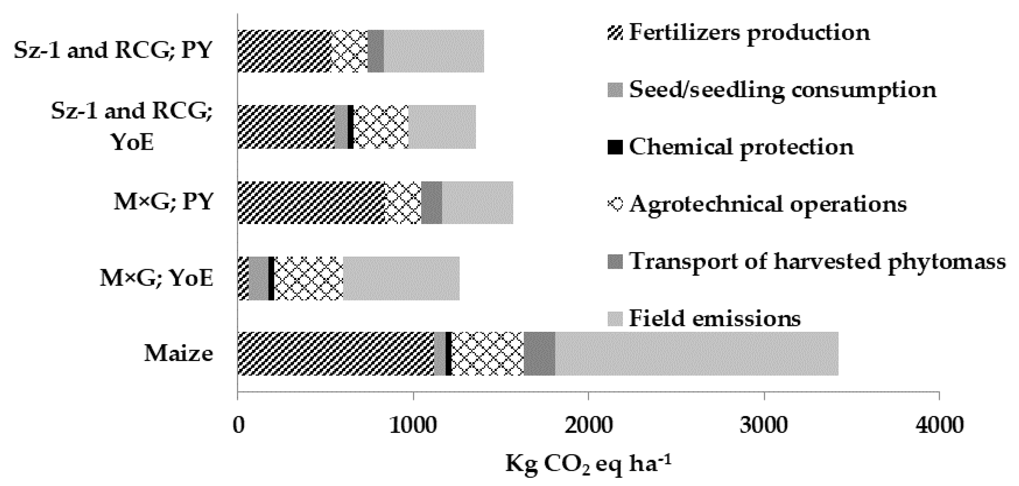
Greenhouse gas emissions per area unit (1 ha) are another monitored aspect and evaluated category. It includes all the material and energy flows for every year. Hectare yield is not included in the evaluation in this case. The category breakdown is shown by the graph in Figure 2. Agricultural production, land use, fertilizers, and energy consumption (from non-renewable resources) in particular contribute significantly to environmental degradation. Increase in biogas efficiency, environmental-friendly farming approaches, and perennial agriculture development are presumed to be the main eventualities [79,80]. Savings in GHC biogas production should be calculated not only per production unit (e.g., kg of CO2 eq GJ−1), which is how most LCA outputs are determined [81], but also per area unit and time unit (MJ/ha/year) [12]. However, many LCA inputs are usually calculated per production unit [81].
Figure 2 shows the major differences in greenhouse gas production per area unit (1 ha) between maize, RCG, Sz-1, and M × G. To incorporate the unique farming technology used for maize into the assessment, any differences between greenhouse gases produced per area unit each year (in accordance with the methodology) were determined. As various farming technologies were employed, the environmental burden of perennial agriculture related to an area unit was divided into several years of establishment (of the crop stand) (YoE) and productive years (PY). The figures in Graph 2 show that conventional maize produces the most emissions per area unit (3422.50 kg of CO2 eq GJ−1). Considering the perennial character of the other crops, models of the environmental burden per area unit were divided into YoE and PY. An area emission burden of 1266.2 kg of CO2 eq GJ−1 in YoE and 1567.7 kg of CO2 eq GJ−1 in PY was quantified for the M × G crop stand establishment in this research. An emission burden of 1358.5 kg of CO2 eq GJ−1 in YoE and 1406.1 kg of CO2 eq GJ-1 in PY was quantified for the Sz-1 and RCG crop stand establishments. Field emissions are the most significant type of emission: during the first four years of our research, maize produced about 1611.9 kg of CO2 eq ha−1 per year, and the perennial crops produced about 384.4–666.9 kg of CO2 eq ha−1 per year, depending on the employed technology. Recalculated to carbon dioxide eq, it reflects the findings of [66,82,83] on clover grasses. Maize imposes a much higher environmental burden than the other tested crops. The environmental burden of maize per area unit is, nevertheless, comparable to the other crops. Generally speaking, and from the point of view of emission burden per area unit, growing perennial crops (Sz-1, RCG, and M × G) is more environmentally-friendly than growing maize. Some other authors have also confirmed this fact, e.g., [46,84]. These crops also provided an adequate yield that is comparable to maize (seen on the long-time horizon).

3.3. Economic Evaluation

A lot of European (e.g., [85,86,87]) as well as Czech (e.g., [17,40,88,89,90], etc.) authors have previously studied and evaluated the economic efficiency of energy crops. It is difficult to compare the results of two different research studies, as they may have applied different methods, preconditions, or frameworks. The following table (Table 19) shows the potential costs of 1 GJ of generated energy, taking the intended use of energy crops into account. Data were collected for almost five years, and the economic balance was determined according to the methodology defined for this research’s purpose (Section 2.3). The economic aspect is the determinant of whether or not a certain crop is included in the cropping, as whether perennial energy crops are accepted by farmers or not depends on their financial profitability [87].
The prices mentioned in this paper are comparable to European standard prices of EUR 5–8 per GJ of energy, as reported in 2009 [87]; nowadays, they are used as indicators of the overall assessment.
Costs per area unit (ha) of maize grown are usually higher than the costs of any other energy crops [91]. However, when comparing costs per unit of generated energy (1 GJ of energy in this case), the situation is the opposite [92] (especially because of a relatively stable and high yield). Our research shows that if phytomass were used in a biogas station, 1 GJ of generated energy would cost EUR 6.1–8.6. Such prices are adequate for the intensity of the growing cycle inputs and for the final phytomass yield (or the potential amount of energy produced). M × G seems to be quite expensive (EUR 8.6 per GJ); this is because the costs of the crop stand establishment are high in this instance, possibly amounting to EUR 2500–4500 per ha, including the preparation of the plot, the purchase of seeds, and the seeding itself [40]. In spite of this, M × G is considered a promising alternative plant. Very desirable economic results may be produced with this crop, depending on the intensity of the inputs and hectare yield [93]. According to our research, Sz-1 and maize seem to be the cheapest options despite intensive maize growing and high input costs (EUR 1150–1350 per ha). Their low costs are due to the annual phytomass yield, which is quite high (14.4 t ha−1 of dry matter on average).
The price of phytomass as a fuel (including transport of phytomass) is highly variable and determined by the fossil fuel market price of energy (including the impact of energy policy and environmental policy). In 2009, unrefined biomass cost EUR 4–5 per GJ in Europe. Heat and energy are mostly generated by biomass made from fast-growing trees and perennial crops [87,94]. The prices of energy phytomass have been varying from EUR 1.4 to 5 per GJ in Europe over the last 15 years [87,88,95]. Such a wide range of prices is caused by different factors, e.g., the biomass market being relatively undeveloped. The price of biomass is largely influenced by the costs of transport and processing methods. The final price of biomass is determined mostly by the input costs (wages, transport, etc.); this is generally applicable to all forms of biomass use. Such costs may be very different in different parts of the Czech Republic. Usually, every form of biomass is used in a different way, and the price of biomass reflects the various forms being used differently. Therefore, the differences in price between stations and forms of biomass are expected to be quite significant in the future [89].
A model of the economic balance was created for the purpose of our research; it is based on the market production of certain energy crops and various intensities of treatment (Table 20).
A subsidy from SAPS (Single Area Payment Scheme) is involved in the model economic balance; it is one of the most stable subsidies that have been provided recently (Table 21). The market price of silage is derived from the current market needs and qualitative parameters of silage material. The price of Sz-1 seeds seems to be quite problematic: it fluctuates, and it is quite high at the moment (up to EUR 27 per kg). Considering a seeding rate of 35 kg per ha, the total seeding costs would amount to EUR 942 (they would rise by 13% in the 10-year cycle).
On the basis of the above results and economic models of market production, we can assess the economic efficiency of growing certain energy crops for the direct sale of phytomass and for the purpose of BGP. After finding a suitable market and sale, we can sell the harvested phytomass efficiently. The market price of harvested phytomass containing 28–36% of dry matter varies from EUR 19 to 46 per ton. Such a price reflects the species and quality, and maize phytomass is usually the most expensive. Table 20, among other data, shows the model’s yearly costs per hectare; they represent the technological costs (total variable costs plus fixed costs of machinery). For the perennial crops, the calculation of the model’s yearly costs is based on the 10-year projection. For the average phytomass yield indicated by this research, the economic profitability would be equal to 9.5–36.9%, and maize would be the most profitable energy crop. The economic efficiency was improved due to the SAPS subsidy, which amounted to EUR 184 per ha, on average, between 2013 and 2016.
The use of grasslands and energy crops without subventions seems to be unrealistic from an economic point of view. The use of available subventions helps a great deal and makes their production economical [96]. In 2006, there were the following subsidies for growing energy crops in the Czech Republic: single area payment scheme (SAPS), additional payment (TOP UP), LFA or NATURA 2000 subsidies, and support for energy crop growing. Nowadays, there is only SAPS, LFA, or NATURA 2000 remaining. Support for energy crop growing (the so-called carbon credit) was terminated in 2009; it is not possible to apply for this kind of payment anymore. In 2006, EUR 43.6 per ha was paid. A farmer had to produce a representative yield in order to gain this kind of support; the representative yield level was stipulated by the Ministry of Agriculture. For example, in 2009, the representative yield was 7 tons per hectare for RCG and 6 tons per hectare for M × G [97].

4. Conclusions

Recently, Sz-1—an alternative and promising energy crop—was introduced in some European countries (mostly in Hungary and Germany), and it has good yield potential. As the results of this research show, Sz-1 produces an average yield that is below a profitable level (≥12 t ha−1 of dry matter) (6.1–8.6 t ha−1, a four-year average). Qualitative analyses for Sz-1 phytomass were performed and show that biogas (or methane) can be made from it, and it produces more energy per production unit than any other energy crop grown in the Czech Republic. The profit from phytomass per area unit and overall economic assessment are crucial factors. According to the findings of this research, and despite its significant environmental benefits, Sz-1 cannot be recommended as an economically viable alternative to maize. Thus, a serious question arises: should the economic or environmental aspect be prioritized?

Author Contributions

J.B.: methodology, software, validation, formal analysis, investigation, resources, data curation, writing—Original draft preparation, writing—Review and editing, visualization, supervision, project administration; M.K.: data curation, methodology; J.M.J.: supervision, methodology, funding acquisition; P.K.: supervision, funding acquisition; Z.Š.: supervision, funding acquisition.

Funding

The research was financially supported by the University of South Bohemia in České Budějovice (project No. GAJU 059/2019/Z).

Conflicts of Interest

The authors declare no conflict of interest.

References

  1. Oslaj, M.; Mursec, B.; Vindis, P. Biogas production from maize hybrids. Biomass Bioenergy 2010, 34, 1538–1545. [Google Scholar] [CrossRef]
  2. Kára, J.; Pastorek, Z.; Přibyl, E.; Hanzlíková, I.; Andert, D.; Gergdtová, I.; Hutla, P.; Měkotová, P.; Abrham, Z.; Mužík, O.; et al. Výroba a Využití Bioplynu v Zemědělství, 1st ed.; Research Institute of Agricultural Engineering: Prague, Czech Republic, 2007; p. 117. [Google Scholar]
  3. Fuksa, P. Netradiční Využití Biomasy v Praxi. Biom.cz [online]. 2009-07-15. Available online: https://biom.cz/cz/odborne-clanky/netradicni-vyuziti-biomasy-v-praxi (accessed on 22 November 2018).
  4. Mužík, O.; Kára, J. Možnosti Výroby a Využití Bioplynu v ČR. Biom.cz [online]. 2009-03-04. Available online: https://biom.cz/cz/odborne-clanky/moznost-vyroby-a-vyuziti-bioplynu-v-cr (accessed on 22 November 2018).
  5. Hijazi, O.; Munro, S.; Zerhusen, B.; Effenberger, M. Review of life cycle assessment for biogas production in Europe. Renew. Sustain. Energy Rev. 2016, 54, 1291–1300. [Google Scholar] [CrossRef]
  6. Agostini, A.; Battini, F.; Giuntoli, J.; Tabaglio, V.; Padella, M.; Baxter, D.; Marelli, L.; Amaducci, S. Environmentally Sustainable Biogas? The Key Role of Manure Co-Digestion with Energy Crops. Energies 2015, 8, 5234–5265. [Google Scholar] [CrossRef]
  7. Lhotský, R.; Kajan, M. Anaerobní digesce fytomasy z trvalých travních porostů jako alternativa k energetickým plodinám. Acta Pruhoniciana 2011, 97, 69–75. [Google Scholar]
  8. Raclavská, H.; Frydrych, J.; Andert, D. Význam Popelovin v Travní Biomase pro Energetické Účely. Biom.cz [online]. 2013-09-23. Available online: https://biom.cz/cz/odborne-clanky/vyznam-popelovin-v-travni-biomase-pro-energeticke-ucely (accessed on 22 November 2018).
  9. Biemans, M.; Waarts, Y.; Nieto, A.; Goba, V.; Jones-Walters, L.; Zöckler, C. Impacts of Biofuel Production on Biodiversity in Europe; ECNC—European Centre for Nature Conservation: Tilburg, The Netherlands, 2008; p. 32. ISBN 978-90-76762-27-2. [Google Scholar]
  10. Dauber, J.; Jones, M.B.; Stout, J.C. The impact of biomass crop cultivation on temperate biodiversity. GCB Bioenergy 2010, 2, 289–309. [Google Scholar] [CrossRef]
  11. Halberg, N.; Hermansen, J.E.; Kristensen, I.S.; Eriksen, J.; Tvedegaard, N.; Petersen, B.M. Impact of organic pig production systems on CO2 emission, C sequestration and nitrate pollution. Agron. Sustain. Dev. 2010, 30, 721–731. [Google Scholar] [CrossRef]
  12. Kočí, V. Na LCA Založené Srovnání Environmentálních Dopadů Obnovitelných Zdrojů Energie, 1st ed.; LCA Studio, Ústav Chemie Ochrany Prostředí, VŠCHT Praha: Dejvice, Czech Republic, 2012; p. 111. [Google Scholar]
  13. ISO. ISO 14040—Environmental management–Life cycle assessment–Principles and framework. International Organization for Standardization: Geneva, Switzerland, 2006. [Google Scholar]
  14. ISO. ISO 14044—Environmental management–Life cycle assessment–Requirements and guidelines; International Organization for Standardization: Geneva, Switzerland, 2006. [Google Scholar]
  15. Ecoinvent. National Life Cycle Inventory database Ecoinvent, Data v1.3; Swiss Centre for Life Cycle Inventories: Dübendorf, Švýcarsko, 2006. [Google Scholar]
  16. Lewandowski, I.; Scurlock, J.M.; Lindvall, E.; Christou, M. The development and current status of perennial rhizomatous grasses as energy crops in the US and Europe. Biomass Bioenergy 2003, 25, 335–361. [Google Scholar] [CrossRef]
  17. Kavka, M.; Beneš, V.; Brant, V. Normativy Zemědělských Výrobních Technologií; Institute of Agriculture Economics and Information: Praha, Czech Republic, 2006; p. 376. [Google Scholar]
  18. Boehmel, C.; Lewandowski, I.; Claupein, W. Comparing annual and perennial energy cropping systems with different management intensities. Agric. Syst. 2008, 96, 224–236. [Google Scholar] [CrossRef]
  19. Wrobel, C.; Coulman, B.E.; Smith, D.L. The potential use of reed canarygrass (Phalaris arundinacea L.) as a biofuel crop. Acta Agric. Scand. Sect. B Soil Plant Sci. 2009, 59, 1–18. [Google Scholar] [CrossRef]
  20. Kukk, L.; Astover, A.; Roostalu, H.; Rossner, H.; Tamm, I. The dependence of reed canary grass (Phalaris arundinacea L.) energy efficiency and profitability on nitrogen fertilization and transportation distance. Agron. Res. 2010, 8, 123–133. [Google Scholar]
  21. Smith, R.; Slater, F.M. The effects of organic and inorganic fertilizer applications to Miscanthus × giganteus, Arundo donax and Phalaris arundinacea, when grown as energy crops in Wales, UK. GCB Bioenergy 2010, 2, 169–179. [Google Scholar] [CrossRef]
  22. Csete, S.; Farkas, Á.; Borhidi, A.; Szalontai, B.; Salamon-Albert, É.; Walcz, I.; Pál, R.W. Tall Wheatgrass Cultivar Szarvasi-1 (Elymus elongatus subsp. ponticus cv. Szarvasi-1) as a Potential Energy Crop for Semi-Arid Lands of Eastern Europe, 1st ed.; INTECH Open Access Publisher: Rijeka, Croatia, 2011; ISBN 978-953-307-408-5. [Google Scholar]
  23. Blengini, G.A.; Brizio, E.; Cibrario, M.; Genon, G. LCA of bioenergy chains in Piedmont (Italy): A case study to support public decision makers towards sustainability. Resour. Conserv. Recycl. 2011, 57, 36–47. [Google Scholar] [CrossRef]
  24. Usťak, S.; Strašil, Z.; Váňa, V.; Honzík, R. Pěstování Chrastice Rákosovité Phalaris arundinacea L. pro Výrobu Bioplynu; Crop Research Institute: Praha, Czech Republic, 2012; p. 24. [Google Scholar]
  25. Strašil, Z. Evaluation of reed canary grass (Phalaris arundinacea L.) grown for energy use. Res. Agric. Eng. 2012, 58, 119–130. [Google Scholar] [CrossRef]
  26. Český Hydrometeorologický Ústav (ČHMÚ). Available online: http://portal.chmi.cz/ (accessed on 17 January 2019).
  27. Bernas, J.; Kopecký, M.; Moudrý, J.; Jelínková, Z.; Konvalina, P. Comparison of germination of selected energy grasses species within different water regimes. Agron. Ser. Sci. Res. Lucr. Stiintifice Ser. Agron. 2014, 57, 29–34. [Google Scholar]
  28. Ecoinvent. Ecoinvent Centre [online]. 2017. Available online: http://www.ecoinvent.org/database/database.htm (accessed on 12 July 2017).
  29. Niggli, U.; Fließbach, A.; Hepperly, P.; Scialabba, N. Low greenhouse gas agriculture: Mitigation and adaptation potential of sustainable farming systems. Ökologie Landbau 2009, 141, 32–33. [Google Scholar]
  30. Gattinger, A.; Muller, A.; Haeni, M.; Skinner, C.; Fliessbach, A.; Buchmann, N.; Niggli, U. Enhanced top soil carbon stocks under organic farming. Proc. Natl. Acad. Sci. USA 2012, 109, 18226–18231. [Google Scholar] [CrossRef] [PubMed]
  31. De Klein, C.; Novoa, R.S.; Ogle, S.; Smith, K.A.; Rochette, P.; Wirth, T.C.; McConkey, B.G.; Mosier, A.; Rypdal, K.; Walsh, M.; et al. N2O emissions from managed soils, and CO2 emissions from lime and urea application. IPCC Guidel. Natl. Greenh. Gas Invent. Prep. Natl. Greenh. Gas Invent. Programme 2006, 4, 1–54. [Google Scholar]
  32. Franks, J.R.; Hadingham, B. Reducing greenhouse gas emissions from agriculture: Avoiding trivial solutions to a global problem. Land Use Policy 2012, 29, 727–736. [Google Scholar] [CrossRef]
  33. Pachauri, R.K.; Allen, M.R.; Barros, V.R.; Broome, J.; Cramer, W.; Christ, R.; Dubash, N.K. Climate Change 2014: Synthesis Report. Contribution of Working Groups I, II and III to the Fifth Assessment Report of the Intergovernmental Panel on Climate Change; IPCC: Geneva, Switzerland, 2014; p. 151. ISBN 978-92-9169-143-2. [Google Scholar]
  34. Forster, P.; Ramaswamy, V.; Artaxo, P.; Berntsen, T.; Betts, R.; Fahey, D.W.; Nganga, J. Changes in Atmospheric Constituents and in Radiative Forcing. In Climate Change 2007; The Physical Science Basis: Cambridge, United Kingdom, 2007; Chapter 2. [Google Scholar]
  35. Solomon, S.; Qin, D.; Manning, M.; Averyt, K.; Marquis, M. Climate Change 2007—The Physical Science Basis: Working Group I Contribution to the Fourth Assessment Report of the IPCC; Cambridge University Press: Cambridge, UK, 2007; Volume 4. [Google Scholar]
  36. Intergovernmental Panel on Climate Change, IPCC. Climate Change 2001: The Scientific Basis; Cambridge University Press: Cambridge, UK, 2001. [Google Scholar]
  37. Exnerova, Z. Agriculture (CRF sector 3). In National Greenhouse Gas Inventory Report Of The Czech Republic (reported inventories 1990–2015), 1st ed.; Krtkova, E., Ed.; Czech Hydrometeorological Institute: Prague, Czech Republic, 2017; p. 491. ISBN 978-80-87577-67-7. [Google Scholar]
  38. Čížková, H.; Rychterová, J.; Hamadejová, L.; Suchý, K.; Filipová, M.; Květ, J.; Anderson, N.O. Biomass production in permanent wet grasslands dominated with Phalaris arundinacea: Case study of the Třeboň basin biosphere reserve, Czech Republic. In The Role of Natural and Constructed Wetlands in Nutrient Cycling and Retention on the Landscape; Springer: Cham, Switzerland, 2015; pp. 1–16. [Google Scholar]
  39. Petříková, V.; Sladký, V.; Strašil, Z.; Šafařík, M.; Usťak, S.; Váňa, J. Energetické Plodiny, 1st ed.; Profi Press: Praha, Czech Republic, 2006; p. 127. [Google Scholar]
  40. Strašil, Z. Základy Pěstování a Možnosti Využití Ozdobnice (Miscanthus), 1st ed.; Crop Research Institute, v.v.i.: Praha, Czech Republic, 2009; p. 52. [Google Scholar]
  41. Menardo, S.; Bauer, A.; Theuretzbacher, F.; Piringer, G.; Nilsen, P.J.; Balsari, P.; Amon, T. Biogas production from steam-exploded miscanthus and utilization of biogas energy and CO2 in greenhouses. Bioenergy Res. 2013, 6, 620–630. [Google Scholar] [CrossRef]
  42. Heaton, E.A.; Boersma, N.; Caveny, J.D.; Voigt, T.B.; Dohleman, F.G. Miscanthus (Miscanthus × giganteus) for biofuel production. Ext. Am. Res. Based Learn. Netw. SUA. Available online: https://articles.extension.org/pages/26625/miscanthus-miscanthus-x-giganteus-for-biofuel-production (accessed on 12 July 2017).
  43. Geißendörfer, H. Perennierende Gräser—Leistungsstarke Alternative zu Energiemais? In Landwirtschaftliches Bildungszentrum Triesdorf [online]. Triesdorf, 2013. Available online: http://www.aelfwb.bayern.de/erwerbskombination/41827/linkurl_0_3.pdf (accessed on 24 February 2014).
  44. Lehtomäki, A.; Viinikainen, T.A.; Rintala, J.A. Screening boreal energy crops and crop residues for methane biofuel production. Biomass Bioenergy 2008, 32, 541–550. [Google Scholar] [CrossRef]
  45. Klimiuk, E.; Pokój, T.; Budzyński, W.; Dubis, B. Theoretical and observed biogas production from plant biomass of different fibre contents. Bioresour. Technol. 2008, 101, 9527–9535. [Google Scholar] [CrossRef] [PubMed]
  46. McEniry, J.; Finnan, J.; King, C.; O’Kiely, P. The effect of ensiling and fractionation on the suitability for combustion of three common grassland species at sequential harvest dates. Grass Forage Sci. 2012, 67, 559–568. [Google Scholar] [CrossRef]
  47. Weiland, P. Production and energetic use of biogas from energy crops and wastes in Germany. Appl. Biochem. Biotechnol. 2003, 109, 263–274. [Google Scholar] [CrossRef]
  48. Amon, T.; Amon, B.; Kryvoruchko, V.; Machmüller, A.; Hopfner-Sixt, K.; Bodiroza, V.; Schreiner, M. Methane production through anaerobic digestion of various energy crops grown in sustainable crop rotations. Bioresour. Technol. 2007, 98, 3204–3212. [Google Scholar] [CrossRef] [PubMed]
  49. Mast, B.; Lemmer, A.; Oechsner, H.; Reinhardt-Hanisch, A.; Claupein, W.; Graeff-Hönninger, S. Methane yield potential of novel perennial biogas crops influenced by harvest date. Ind. Crop. Prod. 2014, 58, 194–203. [Google Scholar] [CrossRef]
  50. Alaru, M.; Olt, J.; Kukk, L.; Luna-delRisco, M.; Lauk, R.; Noormets, M. Methane yield of different energy crops grown in Estonian conditions. Agron. Res. 2011, 9, 13–22. [Google Scholar]
  51. Herrmann, C.; Idler, C.; Heiermann, M. Biogas crops grown in energy crop rotations: Linking chemical composition and methane production characteristics. Bioresour. Technol. 2016, 206, 23–35. [Google Scholar] [CrossRef] [PubMed]
  52. McKendry, P. Energy production from biomass (part 1): Overview of biomass. Bioresour. Technol. 2002, 83, 37–46. [Google Scholar] [CrossRef]
  53. Herrmann, A. Biogas production from maize: Current state, challenges and prospects. 2. Agronomic and environmental aspects. Bioenergy Res. 2013, 6, 372–387. [Google Scholar] [CrossRef]
  54. Weiland, P. Biogas production: Current state and perspectives. Appl. Microbiol. Biotechnol. 2010, 85, 849–860. [Google Scholar] [CrossRef] [PubMed]
  55. Dressler, D.; Loewen, A.; Nelles, M. Life cycle assessment of the supply and use of bioenergy: Impact of regional factors on biogas production. Int. J. Life Cycle Assess. 2012, 17, 1104–1115. [Google Scholar] [CrossRef]
  56. Bacenetti, J.; Negri, M.; Fiala, M.; González-García, S. Anaerobic digestion of different feedstocks: Impact on energetic and environmental balances of biogas process. Sci. Total Environ. 2013, 463, 541–551. [Google Scholar] [CrossRef] [PubMed]
  57. Bernas, J.; Moudry, J., Jr.; Jelinkova, Z.; Kopecky, M.; Konvalina, P.; Moudry, J. Energy crops growing-impact on greenhouse gases emissions. J. Environ. Prot. Ecol. 2016, 17, 950–960. [Google Scholar]
  58. Bernas, J.; Moudrý, J., Jr.; Jelinkova, Z.U.; Kopecky, M.A. Greenhouse gasses emissions during maize growing for energy purposes. In MendelNet 2014; Mendelu: Brno, Czech Republic, 2014; pp. 219–223. ISBN 978-80-7509-174-1. [Google Scholar]
  59. Mosier, A.R. Soil processes and global change. Biol. Fertil. Soils 1998, 27, 221–229. [Google Scholar] [CrossRef]
  60. Van Zeijts, H.; Leneman, H.; Sleeswijk, A.W. Fitting fertilisation in LCA: Allocation to crops in a cropping plan. J. Clean. Prod. 1999, 7, 69–74. [Google Scholar] [CrossRef]
  61. Zou, J.; Huang, Y.; Lu, Y.; Zheng, X.; Wang, Y. Direct emission factor for N2O from rice–winter wheat rotation systems in southeast China. Atmos. Environ. 2005, 39, 4755–4765. [Google Scholar] [CrossRef]
  62. Mori, A.; Hojito, M.; Kondo, H.; Matsunami, H.; Scholefield, D. Effects of plant species on CH4 and N2O fluxes from a volcanic grassland soil in Nasu, Japan. Soil Sci. Plant Nutr. 2005, 51, 19–27. [Google Scholar] [CrossRef]
  63. Mancinelli, R.; Marinari, S.; Di Felice, V.; Savin, M.C.; Campiglia, E. Soil property, CO2 emission and aridity index as agroecological indicators to assess the mineralization of cover crop green manure in a Mediterranean environment. Ecol. Indic. 2013, 34, 31–40. [Google Scholar] [CrossRef]
  64. Moudrý, J., Jr.; Jelínková, Z.; Plch, R.; Moudrý, J.; Konvalina, P.; Hyšpler, R. The emissions of greenhouse gases produced during growing and processing of wheat products in the Czech Republic. J. Food Agric. Environ. 2013, 11, 1133–1136. [Google Scholar]
  65. Smith, P.; Martino, D.; Cai, Z.; Gwary, D.; Janzen, H.; Kumar, P.; Scholes, B. Greenhouse gas mitigation in agriculture. Philos. Trans. R. Soc. B Biol. Sci. 2008, 363, 789–813. [Google Scholar] [CrossRef] [PubMed]
  66. Šimek, M.; Macková, J. Degradace Půdy a Emise Skleníkových Plynů z půd a ze Zemědělství—Nutné Zlo? 1st ed.; Středisko Společných Činností AV ČR, v.v.i.: Strategie AV21/Rozmanitost Života a Zdraví Ekosystémů: Prague, Chzech Republic, 2015; p. 46. [Google Scholar]
  67. Bos, J.F.; de Haan, J.; Sukkel, W.; Schils, R.L. Energy use and greenhouse gas emissions in organic and conventional farming systems in the Netherlands. NJAS-Wagening. J. Life Sci. 2014, 68, 61–70. [Google Scholar] [CrossRef]
  68. LaSalle, T.J.; Hepperly, P. Regenerative Organic Farming: A Solution to Global Warming; Rodale Institute: Berks County, PA, USA, 2008; pp. 1–13. [Google Scholar]
  69. Grieder, C.; Dhillon, B.S.; Schipprack, W.; Melchinger, A.E. Breeding maize as biogas substrate in Central Europe: I. Quantitative-genetic parameters for testcross performance. Theor. Appl. Genet. 2012, 124, 971–980. [Google Scholar] [CrossRef] [PubMed]
  70. Sauerbeck, D.R. CO2 emissions and C sequestration by agriculture–perspectives and limitations. Nutr. Cycl. Agroecosyst. 2001, 60, 253–266. [Google Scholar] [CrossRef]
  71. Küstermann, B.; Kainz, M.; Hülsbergen, K.J. Modeling carbon cycles and estimation of greenhouse gas emissions from organic and conventional farming systems. Renew. Agric. Food Syst. 2008, 23, 38–52. [Google Scholar] [CrossRef]
  72. Moudry, J.; Jirouskova, Z.; Plch, R.; Konvalina, P.; Hyspler, R. Emisní zátěž při pěstování a zpracování pšenice. Úroda Časopis Pro Rostl. Prod. 2011, 59, 501–506. [Google Scholar]
  73. Moudry, J.; Jirouskova, Z.; Konvalina, P. Pěstitelské technologie a emise CO2 The Cultivation Technologies and Emission of CO2. Uroda 2010, 58, 725–728. [Google Scholar]
  74. Dorninger, M.; Freyer, B. Aktuelle Leistungen und Zukünftige Potentiale der Ökologischen Landwirtschaft für den Klimaschutz in Österreich, 1st ed.; IFOL, BOKU: Wien, Austria, 2008; p. 36. [Google Scholar]
  75. Pottebaum, P.; Bullerdiek, A. Handbuch Direkt-Vermarktung., 1st ed.; Verlag Unions Agrar: Münster, Germany, 1994; 376p. [Google Scholar]
  76. Stratmann, B.; Teufel, J.; Wiegmann, K. Umweltauswirkungen von Ernährungsgewohnheiten, 1st ed.; Öko-Institut eV.: Freiburg, Germany, 2008; p. 15. [Google Scholar]
  77. Moudrý, J., Jr.; Moudrý, J. Environmental Aspects of Organic Farming, 1st ed.; Intech: London, UK, 2014; Chapter 11; 28p. [Google Scholar]
  78. Eurostat. Early Estimates of CO2 Emissions from Energy Use in 2016, CO2 Emissions in the EU Estimated to Have Slightly Decreased Compared with 2015 [online]. Eurostat Press Office, 2017. Available online: http://ec.europa.eu/eurostat/documents/2995521/8010076/8-04052017-BP-EN.pdf/7b7462ca-7c53-44a5-bafb-23cc68580c03 (accessed on 4 May 2017).
  79. Serafínová, C. Možnosti Aplikace Metody LCA pro Energetické Procesy Využívající Odpadní Biomasu. Biom.cz [online]. 2009-06-03. Available online: http://biom.cz/cz/odborne-clanky/moznosti-aplikace-metody-lca-pro-energeticke-procesy-vyuzivaji-odpadni-biomasu (accessed on 7 June 2016).
  80. Jury, C.; Benetto, E.; Koster, D.; Schmitt, B.; Welfring, J. Life cycle assessment of biogas production by monofermentation of energy crops and injection into the natural gas grid. Biomass Bioenergy 2010, 34, 54–66. [Google Scholar] [CrossRef]
  81. Roy, P.; Nei, D.; Orikasa, T.; Xu, Q.; Okadome, H.; Nakamura, N.; Shiina, T. A review of life cycle assessment (LCA) on some food products. J. Food Eng. 2009, 90, 1–10. [Google Scholar] [CrossRef]
  82. Flessa, H.; Ruser, R.; Dörsch, P.; Kamp, T.; Jimenez, M.A.; Munch, J.C.; Beese, F. Integrated evaluation of greenhouse gas emissions (CO2, CH4, N2O) from two farming systems in southern Germany. Agric. Ecosyst. Environ. 2002, 91, 175–189. [Google Scholar] [CrossRef]
  83. Šimek, M.; Elhottová, D.; Klimeš, F.; Hopkins, D.W. Emissions of N2O and CO2, denitrification measurements and soil properties in red clover and ryegrass stands. Soil Biol. Biochem. 2004, 36, 9–21. [Google Scholar] [CrossRef]
  84. Bellarby, J.; Foereid, B.; Hastings, A. Cool Farming: Climate Impacts of Agriculture and Mitigation Potential, 1st ed.; Greenpeace International: Amsterdam, The Netherland, 2008; p. 44. [Google Scholar]
  85. Hanegraaf, M.C.; Biewinga, E.E. Assessing the ecological and economic sustainability of energy crops. Biomass Bioenergy 1998, 15, 345–355. [Google Scholar] [CrossRef]
  86. BoÈrjesson, P. Erratum to Environmental effects of energy crop cultivation in Sweden Ð II: Economic evaluation [Biomass and Bioenergy 16 (1999) 155]. Biomass Bioenergy 1999, 16, 1. [Google Scholar]
  87. Ericsson, K.; Rosenqvist, H.; Nilsson, L.J. Energy crop production costs in the EU. Biomass Bioenergy 2009, 33, 1577–1586. [Google Scholar] [CrossRef]
  88. Strašil, Z.; Moudrý, J.; Kalinová, J. Produkce a ekonomika vybraných energetických rostlin. In Sborník z Konference Udržatěl’né pol’nohospodárstvo a Rozvoj Vidieka, 1st ed.; Slovak University of Agriculture in Nitra: Nitra, Slovak Republic, 2003; pp. 333–335. [Google Scholar]
  89. Havlíčková, K.; Weger, J.; Boháč, J.; Štěrba, Z.; Hutla, P.; Knápek, J.; Vašíček, J.; Strašil, Z.; Kajan, M.; Lhotský, R. Rostlinná Biomasa Jako Zdroj Energie, 1st ed.; VUKOZ Pruhonice: Průhonice, Czech Republic, 2008; p. 83. [Google Scholar]
  90. Ochodek, T.; Koloničný, J.; Janásek, P. Potenciál Biomasy, Druhy, Bilance a Vlastnosti Paliv z Biomasy, 1st ed.; Energy Research Center VŠB, Technical University of Ostrava: Ostrava, Czech Republic, 2006; p. 24. [Google Scholar]
  91. Idel, S. Energiegras Soll Mais Ersetzen. [online] 2013. Available online: http://www.nwzonline.de/oldenburg-kreis/wirtschaft/energiegras-soll-mais-ersetzen_a_6,2,739225373.html (accessed on 9 February 2018).
  92. Markou, G.; Brulé, M.; Balafoutis, A.; Kornaros, M.; Georgakakis, D.; Papadakis, G. Biogas production from energy crops in northern Greece: Economics of electricity generation associated with heat recovery in a greenhouse. Clean Technol. Environ. Policy 2017, 19, 1147–1167. [Google Scholar] [CrossRef]
  93. Zimmermann, J.; Styles, D.; Hastings, A.; Dauber, J.; Jones, M.B. Assessing the impact of within crop heterogeneity (‘patchiness’) in young Miscanthus × giganteus fields on economic feasibility and soil carbon sequestration. GCB Bioenergy 2014, 6, 566–576. [Google Scholar] [CrossRef]
  94. Lewandowski, I.; Clifton-Brown, J.C.; Scurlock, J.M.O.; Huisman, W. Miscanthus: European experience with a novel energy crop. Biomass Bioenergy 2000, 19, 209–227. [Google Scholar] [CrossRef]
  95. Havlíčková, K.; Weger, J.; Konvalina, P.; Moudrý, J.; Strašil, Z. Zhodnocení Ekonomických Aspektů Pěstování a Využití Energetických Rostlin. Vědecká Monografie, 1st ed.; Výzkumný ústav Silva Taroucy pro krajinu a okrasné zahradnictví Průhonice a Jihočeská univerzita v Českých Budějovicích, Zemědělská fakulta: Ceske Budejovice, Czech Republic, 2007; p. 92. [Google Scholar]
  96. Abrham, Z.; Kovářová, M.; Ferienčiková, D.; Kizeková, M.; Ondrášek, L.; Zimková, M. Economy of biomass from grass stands. In Proceedings of the Medzinárodná Vedecká Konferencia pri Príležitoti 70 Výročia Krmivinárskeho Výskumu na Slovensku, Trávne Porasty-Súčast´ Horského Pol’nohospodárstva a Krajiny, Banská Bystrica, Slovakia, 27–28 September 2006; Grassland and Mountain Agriculture Research Institute: Banská Bystrica, Slovakia, 2006; pp. 1–8. [Google Scholar]
  97. Bednár, J. Podpora Obnovitelných Zdrojů Energie v Agrárním Sektoru. Biom.cz [online]. 2009-07-08. Available online: http://biom.cz/cz/odborne-clanky/podpora-obnovitelnych-zdroju-energie-v-agrarnim-sektoru (accessed on 8 September 2017).
Figure 1. Contributions of every process to the total environmental burden (%).Identical contribution of RCG and Sz-1 and every process to the total environmental burden (%) is caused by identical farming technology used.
Agronomy 09 00098 g001
Figure 2. Emissions per area unit. PY = productive year, YoE = year of establishment.
Agronomy 09 00098 g002
Table 1. Temperature and precipitation characteristics—České Budějovice (modified from [26]).
YearAverage Temperature (°C)Precipitation (mm)
YearSeasonYearSeason
20129.315.3798.1567.7
20139.115.3685.4469.5
201410.215.1595.9428.7
201510.516.9487.7233.8
201610.515.7680.9447.7
20179.716.4630.3438.8
Average (2012–2017)9.915.8646.4431.0
Long-term average (1961–1990)8.214.2582.8366.2
Season (i.e., growing season) includes April, May, June, July, and August.
Table 2. The station characteristics (modified from [26]).
Parameters
Altitude (MAMSL)380
Agricultural production regionCereal production
Soil texture classSand-loamy class
Soil typePseudogley Cambisol
Soil pH6.4
Long-term average temperature (°C)8.2
Long-term seasonal rainfall (mm)366.2
Global Positioning System (GPS) coordinates48° 57′ 07″ N; 14° 28′ 17″ E
Table 3. Methodology of fertilization in a year when the crop stand was established.
Used Nutrients (kg ha−1)
Nitrogen (N)Phosphorus (P)Potassium (K)
PureFertilizer and Its AmountPure/OxideFertilizer and Its AmountPure/OxideFertilizer and Its Amount
Sz-167AS 200, AN 10048 (135 of P2O5)SF3 30030 (37.5 of K2O)PS 62.5
RCG67AS 200, AN 10048 (135 of P2O5)SF3 30030 (37.5 of K2O)PS 62.5
Doses of fertilizers were identical every year when the crop stands were established. Sz-1 and RCG see Section 1; AS, AN, SF3, PS see section “Szarvasi-1 and Reed Canary Grass”.
Table 4. Methodology of fertilization in productive years.
Used Nutrients (kg ha−1)
Nitrogen (N)Phosphorus (P)Potassium (K)
PureFertilizer and Its AmountPure/OxideFertilizer and Its AmountPure/OxideFertilizer and Its Amount
Sz-1100AS 300, AN 15010 (28.2 of P2O5)SF3 62.530 (37.5 of K2O)PS 62.5
RCG100AS 300, AN 15010 (28.2 of P2O5)SF3 62.530 (37.5 of K2O)PS 62.5
Table 5. Overview table for Miscanthus × Giganteus.
Year of SeedingDensity of Rhizomes (m)FertilizersDepth of Plants Seeded (cm)Area (sq. meters)
20130.5 × 1Mineral8–10100
Table 6. Methodology of fertilization of Miscanthus × Giganteus applied in productive years.
Used Nutrients (kg ha−1)
Nitrogen (N)Phosphorus (P)Potassium (K)
PureFertilizer and Its AmountPure/OxideFertilizer and Its AmountPure/OxideFertilizer and Its Amount
M × G70AN 26040 (112.5 of P2O5)SF3 25070 (87 kg of K2O)PS 145
The intensity of fertilization of M × G was derived from typical intensive farming methods. M × G crop stands are not usually fertilized in the first crop stand establishment.
Table 7. Methodology of fertilization of maize.
MaizeUsed Nutrients (kg ha−1)
Nitrogen (N)Phosphorus (P)Potassium (K)
PureFertilizer and its amountPure/oxideFertilizer and its amountPure/oxideFertilizer and its amount
150U 32530 (85.5 of P2O5)SF3 19050 (62.4 of K2O)PS 104
The intensity of fertilization of maize was derived from typical intensive farming methods.
Table 8. Inventory table: inputs and outputs of life cycle.
Standard Conventional Farming Technology
OutputUnitSz-1RCGM × GMaize
GJaverage energy gain (GJ ha−1)
InputUnit
Inputs from technosphere Sz-1RCGM × GMaize
Ammonium nitrate (as N)kgxxxx
Ammonium sulphate (as N)kgxx
Application of plant protection products by field sprayerhaxxxx
Combined harvestinghaxxxx
Fertilization by broadcasterhaxxxx
Glyphosatekgxxxx
Grass seedkgxx
Herbicide at plantkgxxxx
Maize seed for sowingkg x
Manure, solid, cattlekg xx
Miscanthus rhizome for plantingp x
Nitrogen fertilizer (as N), urea ammonium nitrate productionkg x
Plantingha x
Potassium chloride (as K2O)kgxxxx
Solid manure loading and spreading by hydraulic loader and spreaderkg xx
Sowinghaxx x
Tillage, harrowing by rotary harrowhaxxxx
Tillage, harrowing by spring tine harrowhaxxx
Tillage, plowinghaxxxx
Tillage, rollinghax xx
Transport, tractor, and trailer, agriculturaltkmxxxx
Triple superphosphate (as P2O5)kgxxxx
Inputs from nature
Land occupationhaxxxx
Inputs in the air
Carbon dioxide (from fertilizers)IPCCkgx
Dinitrogen monoxide (from fertilizers)IPPCkgxxxx
Inventory of input and output data; × = input from Ecoinvent 3 database; calculated in accordance with the IPCC (Intergovernmental Panel on Climate Change) methodology (Section “Determination of Field Emissions”).
Table 9. Summary of final figures: average harvest used for BGP.
CropDry Matter (t ha−1)CH4 (m3)Energy (GJ ha−1)Area Needed for Generating the Same Energy Gain (ha)kg CO2 eq GJ−1 4-Year Averagekg CO2 eq GJ−1 10-Year Average
Maize14.45981214.1116.013.3
M × G9.63422122.51.716.28.1
RCG8.62920104.52.016.97.6
Sz-18.63171113.51.915.67.2
Average yield of phytomass does not include the first non-productive year—the one in which the crop stand is established (compared with the average emission load).
Table 10. LSD (Least Significant Difference) test: impact of species on average yield of phytomass (kg ha−1) and on average energy efficiency (GJ ha−1).
Homogeneous Groups, alpha = 0.05
Error: Intergroup. AS = 12180000, df = 44.00
Homogeneous Groups, alpha = 0.05
Error: Intergroup. AS = 2408.0, df = 44.00
SpeciesAverage yield of phytomassAverage energy efficiency
Maize14,457.71b215.28b
M × G9622.67a122.30a
RCG8582.20a104.53a
Sz-18635.61a113.56a
Rem.: AS = average square; values indicated by the same letter do not show any statistically significant differences at a level of significance of p < 0.05; df = degrees of freedom
Table 11. One-dimensional tests of significance for the average yield of phytomass (kg ha−1) and the average energy efficiency (GJ ha−1) (ANOVA analysis).
Average Yield of PhytomassAverage Energy Efficiency
FactordfAS%dfAS%
Species (1)39.38 ***33.87331,728.1 ***63.86
Year (2)28.97 *32.3922669.0 ***5.37
1*2fc67.55 ***27.27614,983.3 ***30.16
Error361.796.4736297.60.61
Rem.: df = degree of freedom; AS = average square; * = statistically significant, p ≤ 0.05; *** = statistically significant, p ≤ 0.001; fc = factor combination; df = degrees of freedom.
Table 12. Dates of mow of perennial crops and maize.
Date of MowI.II. (Harvest of Maize)
2013-15 September
20146 June30 September
201512 June1 October
20162 June13 September
Perennial crops were harvested in two phases. Perennial crop stands were not mowed in the first year.
Table 13. Average dry matter content in phytomass at the moment of harvest (%).
Sz-1RCGM × GMaize
Average dry matter content in phytomass at the moment of harvest (%)38.340.036.336.7
Table 14. LSD test: average dry matter content (kg ha−1) in perennial crops (RCG, Sz-1, M × G) during every mow.
Homogeneous Groups, Alpha = 0.05000. Error: Intergroup. AS = 3825000, df = 166.00
Mowaverage dry matter yield
14961 b
22932 a
Rem.: AS = average square; values indicated by the same letter do not show any statistically significant differences at p < 0.05; df = degrees of freedom.
Table 15. Results of assessment of silage samples.
Sz-1RCGM × GMaize
CH4 (l kg−1 of dry matter)367.2340.3355.0416.0
CH4 (l kg−1 of sample)94.9102.370.2127.7
CH4 (l kg−1 of organic dry matter)410.7377.4414.7434.6
Burnt heat (MJ kg−1 of dry matter)14.613.514.116.6
Calorific value (MJ kg−1 of dry matter)13.112.212.714.9
Dry matter (g kg−1 of sample)240.50288.00208.30283.20
Nitrogenous elements (g kg−1 of sample)23.8922.3620.5419.89
Fiber (g kg−1 of sample)71.4075.8574.0856.02
Ash (g kg−1 of sample)30.7830.3717.3112.14
Lactic acid (g kg−1 of sample)19.5422.204.5017.48
Acetic acid (g kg−1 of sample)3.843.203.872.15
Butyric acid (g kg−1 of sample)0.000.000.000.00
Values come from the analyses performed in accordance with the methodology described in Section 2.2.
Table 16. CH4 yield depending on phytomass yield (m3 of CH4, Σ for 4 years).
m3 of CH4, 4-Year Sum
Maize23,922.1
M × G10,264.5
RCG8761.0
Sz-19512.7
Table 17. Average values of volume weight.
Sz-1RCGM × GMaize
Volume weight (kg m³)577.1505.8527.7752.1
Table 18. Emission load (kg of CO2 eq) according to the production unit (GJ).
System SubprocessesMaizeM × GRCGSz-1
Organic fertilizers0.290.17xx
Mineral fertilizers N4.145.015.535.10
Mineral fertilizers P0.651.491.131.04
Mineral fertilizers K0.130.330.220.20
Seed consumption0.310.310.220.21
Chemical protection0.160.100.110.10
Agrotechnological operations1.932.722.192.02
Transport of harvested phytomass0.841.020.870.84
Field emissions7.535.066.596.07
Total environmental burden15.9916.1816.8815.58
All energy inputs entering the system in the first 4 years are included in the system processes.
Table 19. Price of to 1 GJ of generated energy.
MaizeM × GRCGSz-1
EUR GJ−16.18.67.06.4
Table 20. Model economic balance based on the market production.
Phytomass Growing for the BGP (Biogas Plant) Purpose
Year costs per hectare (EUR per ha)Average silage yield (t per ha)Silage market price (EUR per t)Potential profit (EUR per ha)+ SAPS subsidy (EUR per ha)
Maize1305.846.4819.2–38.5481.9665.8
M × G1055.532.1326.9–38.5180.2364.1
RCG728.223.5226.9–38.5176.4360.3
Sz-1728.224.6626.9–38.5220.3404.2
Single value of EUR (Euros) 38.5 per ton is considered the market price of silage; the amount of SAPS subsidy derives from the average for 2013–2016
Year hectare costs represent the technological costs (total variable costs + fixed costs of machinery), and for perennial crops, they are based on 10-year projection.
Table 21. Development subsidies from the SAPS.
YearSAPS Subsidy (EUR per ha)
2012224.5
2013233.4
2014230.7
2015136.3
2016135.2
average for 2013–2016183.9
(SAPS: Single Area Payment Scheme).

