CFD Models as a Tool to Analyze the Performance of the Hydraulic Agitation System of an Air-Assisted Sprayer

Abstract

A computational fluid dynamics (CFD) model of the fluid velocities generated by the agitation system of an air-assisted sprayer was developed and validated by practical experiments in a laboratory. The model was developed considering different settings of the agitation system: Three water levels in the tank (1000, 2000, and 3000 L); two different numbers of active nozzles (2 or 4); and three working pressures of the agitation circuit (8, 10, or 12 bar). Actual measurements of the fluid velocity into the tank were taken using an acoustic Doppler velocimeter (ADV). CFD simulations made it possible to estimate fluid velocities at 38% of the measuring points with relative errors of less than 30%. Additionally, the CFD models have allowed the correct prediction of the general behavior of the fluid in the tank considering mean velocities depending on the setting parameters of the agitation system (water level in the tank, hydraulic circuit pressure, and number of active nozzles).

1. Introduction

The application of plant protection products (PPPs) in agricultural crops requires its appropriate dissolution in water to achieve a successful treatment according to the established prescriptions. For this goal, the tanks of the agricultural sprayers are equipped with agitation systems that should ensure a homogeneous PPP concentration in the tank, avoiding sedimentation.

Most sprayers have hydraulic agitation systems based on the use of injection nozzles. These systems consist of one or several nozzles (jet agitation systems) that, working at a specific pressure, introduce a liquid flow rate into the tank, generating turbulent flow. The mixing quality depends on different factors, including the geometry of the tank, quantity of water in the tank, nozzle location, nozzle flow rate, system pressure, and the time available for mixing.

To analyze the quality of the agitation, the standardized procedure ISO 5682-2 [1], which specifies the methods of testing and assessing the performance of agitation systems in hydraulic sprayers, can be used. This standard requires the collection of samples at various points in the tank and at the spraying nozzles, for laboratory measurement of the concentration of active matter. Performing these tests is time consuming and requires important material resources. In addition, information obtained for each test is specific according to the control parameters: Pressure of the agitation system, number of nozzles, water level, etc. In addition, results are not easily extrapolated to other regulation conditions of the agitation system.

As an alternative to the standardized procedure ISO 5682-2, different methodologies have been proposed such as the use of devices to measure liquid turbulence in the tank [2,3,4,5], image analysis using tanks with transparent walls [6], and the use of instrumentation to measure fluid velocity inside the tank [2,7]. In addition to experimental measurements, numerical models based on the use of computational fluid dynamics (CFD) have also been applied [8].

In this sense, the study of agitation systems should allow for the analysis of the effect of set variables (pressure, number of nozzles, nozzle flow, nozzle position, liquid level in the tank) on the concentration of active ingredients in the sample. Performing this type of study according to the ISO 5682-2 standard, for different pressure configurations, nozzle types, etc., would be prohibitively expensive and time consuming; instead, the sprayer’s manufacturers require rapid measurement methods that can validate the modeling carried out in the design phase. An ideal experimental test method would be one that provides information to allow manufacturers to quantify the same parameters used by engineers in the design phase, which, in most cases, are the estimated flow velocity at different points of the sprayer tank by using computational fluid dynamics. For this purpose, different studies have investigated fluid velocities inside spray tanks using CFD, and these values have been validated by experimental measures [9,10]. As an additional step in this line of work, some researchers [11] CFD-modeled the movement of fluid in a 4000 L tank of an agricultural sprayer and attempted to correlate the velocity of the fluid with the concentration of active ingredient, obtaining inconclusive results. Xiongkuy et al. [12] concluded that the efficacy of agitation was improved by increases in both flow rate and working pressure; similar conclusions were obtained by Tamagnone et al. [6]. In turn, it can be concluded that an increase in fluid velocity will produce an improvement in the efficacy of the agitation system [7].

The empirical measurement of fluid velocities inside the tank can be carried out using different systems such as particle image velocimeters [13], laser Doppler velocimeters [10], hot-film anemometers [9], acoustic Doppler velocimeters (ADV) [7,14], electromagnetic current meters [15], and electronic flow meters [2]. In most cases, acoustic Doppler velocimetry has been the preferred method [13,16,17] because it is relatively low in cost, can record at a relatively high frequency (up to 100 Hz), can measure three-dimensional instantaneous velocities, and is nonintrusive because it has a relatively small sampling volume according to the instrument selected. Furthermore, calibration is invariant [15].

Therefore, the objective of this work was to study the applicability of CFD models to validate the fluid velocities obtained by using an ADV to investigate the operation and efficiency of a hydraulic agitation system in the tank of an air blast sprayer according to different working parameters. Specific information of the methodology and results of the measurements made using an ADV are detailed in García-Ramos et al. [7].

2. Materials and Methods

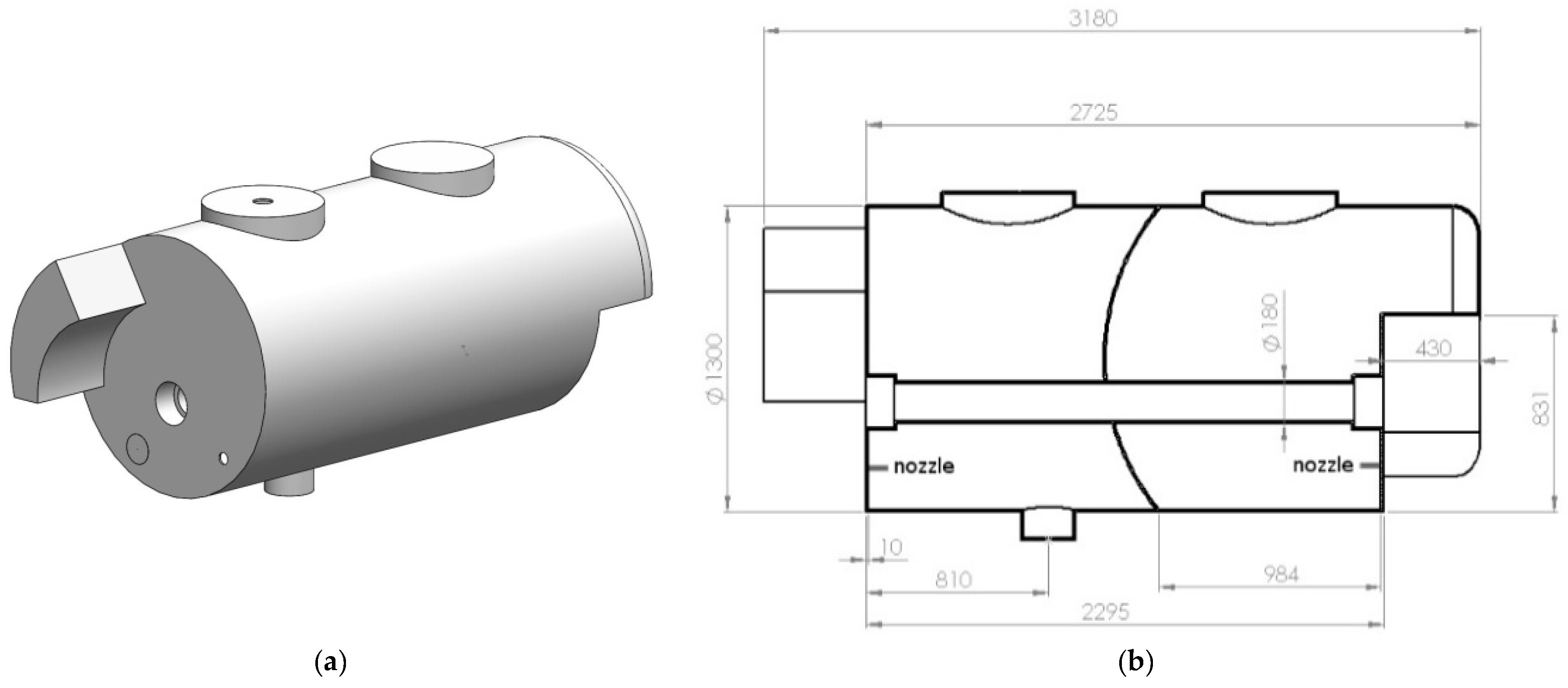
2.1. Agricultural Sprayer

This study was carried out using an air-assisted sprayer with a nominal capacity of 3000 L (GarMelet S.L.). The geometry of the tank was cylindrical and the inside was divided into two interconnected parts (Figure 1). The agitation system consisted of four Venturi nozzles placed on the bottom of the opposite sides of the cylinder, two on each side. The inside geometry of the tank is shown in Figure 1.

2.2. Fluid Velocity Measurements

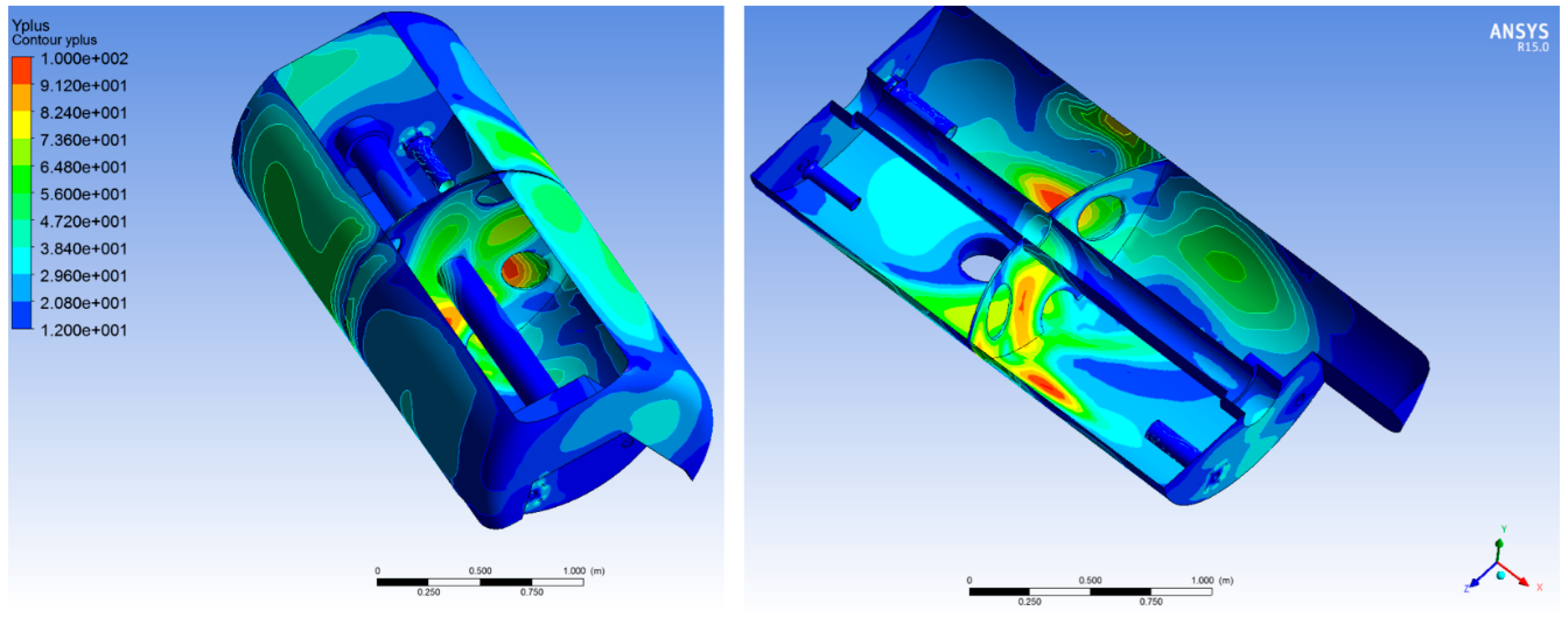
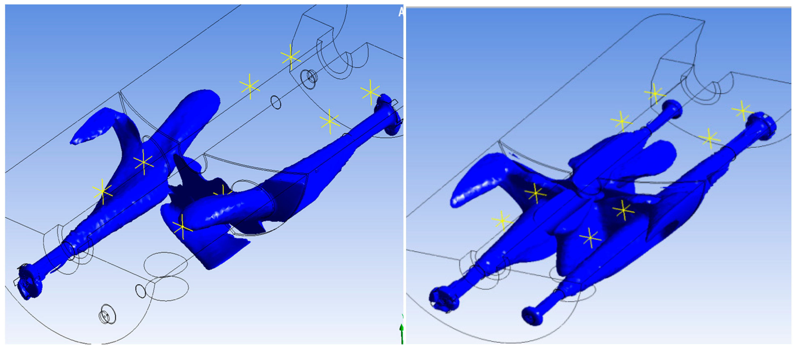
An experimental factorial design was carried out with 3 independent variables for the configuration of the agitation system: Water level in the tank (1000, 2000, or 3000 L); number of active nozzles (2 or 4); and working pressure of the agitation circuit (8, 10, or 12 bar).

Velocity measurements were made in four circular sections of the tank, with eight measuring points in each section distributed at three heights (Figure 2). These measurements were carried out considering the different combinations of the variables (pressure, number of nozzles, and tank filling level). When the system worked with two nozzles, these were on opposite sides of the tank.

In this sense, considering 1000 L in the tank, measurements could only be taken at points 1 and 2 (Figure 2), whereas with 2000 L, they could be taken only at points 1, 2, 3, 4, and 5. Measurements at all sampling points were, therefore, only available with 3000 L of water in the tank.

A 3D microacoustic Doppler velocimeter (3D MicroADV 16MHz by Sontek, San Diego, CA, USA) was used to carry out the velocity measurements, according to the methodology described in [7]. For the validation, 18 CFD models were developed (3 water levels × 2 number of nozzles × 3 working pressures).

2.3. CFD Model

A CFD simulation software, specifically, the commercial ANSYS-Fluent v. 15 (ANSYS, Inc., Canonsburg, PA, USA), widely accepted by the scientific community for numerical fluid simulations, was used to analyze the liquid velocities generated in the tank sprayer.

The geometry of the tank was drawn with a CAD program. Later, the geometry was imported to a meshing module (Meshing-ANSYS ICEM CFD). In this module, aspects such as the size of the cells or the meshing close to the walls of the model are controlled. It is also possible to predetermine the boundary conditions of the model. Finally, the mesh was imported into the ANSYS-FLUENT program, where the final configuration and calculation were performed.

Of the calculation configuration parameters, the first is to specify whether the calculation is transient or stationary. In our case, the stationary option was chosen, as it represents the reality of the experimental test (constant volume of liquid in the tank and machine stopped in the laboratory).

Secondly, we are faced with the problem of modeling the air in the upper part of the tank not occupied by liquid. ANSYS-FLUENT has multiphase models that would allow a faithful modeling of the liquid–air interphase in the tank, but it would require a great deal of computing power. As, moreover, air does not intervene in the problem, a simple solution was chosen: Only model the water. In this way, it is possible to have a single-phase mode, improving the model convergence.

This methodology has, as a main inconvenience, the requirement of developing a different mesh model for each water volume setting in the tank (Figure 3).

In other words, a model in which different phases could be implemented would allow the same mesh to be used for any volume of water in the tank, but it would require a great deal of computing power. On the contrary, it is advantageous to develop several simpler models, provided that the goal of the research is only obtaining the liquid velocities inside the tank. In this sense, one simplification must be assumed: The waves inside the tank are negligible.

In our case, having analyzed the tank with liquid volumes of 1000, 2000, and 3000 L, 3 different meshes were developed, which are described in

Table 1. Characteristics of the computational fluid dynamics (CFD) mesh models developed.

	1000 L Mesh	2000 L Mesh	3000 L Mesh
Number of cells	965,063	1,494,857	1,046,289
Minimum cell size	4.42 × 10−4 m	4.55 × 10−4 m	4.75 × 10−4 m
Maximum cell size	0.025 m	0.025 m	0.035 m
Mesh type	unstructured
Meshed in walls	6 layers

. Previously, to decide the meshes used in the simulations, a mesh convergence study was carried out [18] for the case of 2 nozzles and 10 bar in which several meshes (cell sizes of 50, 35, and 25 mm) were tested for the three levels of water in the tank (

Table 2. Characteristics of the CFD meshes studied previously (2 nozzles, 10 bar). * Meshes finally developed in the numerical model selected.

	Maximum Cell Dimension (mm)
Tank level (L)	25	35	50
1000	965,063 *	578,617	485,779
2000	1,494,857 *	772,332	574,015
3000	2,142,219	1,046,289 *	670,288

). No relevant differences were found between results compared to different meshes. To establish the meshes in the walls, values of y⁺ obtained in these previous calculations were analyzed. It was observed that almost all the walls had values of y⁺ between 12 and 100 (Figure 4). As an exception, the vertical walls of the ends (not the internal breakwater) and the cylinder surrounding the axis of the power take-off, whose values of y⁺ were below 10. In view of the results, it was decided to use the scalable wall model in the final calculations, because, in this way, the program guarantees that the calculated y⁺ does not fall below 11,125 (limit between the viscous and turbulent layer); nevertheless, the influence of the vertical walls in the data obtained in the measurement points is limited as no differences were found between the use of standard or scalable wall functions.

One of the problems presented by this simplification is the modeling of the water-free sheet in the tank. The “wall” contour condition cannot be imposed, but neither is this surface a fluid outlet. As a proposal, it has been decided to impose a fluid inlet condition, specifying that the mass of fluid entering through that contour is zero.

The other boundary conditions are more evident: The nozzles are considered liquid inlets; the Venturi nozzles of the agitation system were modeled considering their actual geometry and nominal flow at different working pressures.

The outlet boundary condition, necessary for the calculation of the models, was arranged at the bottom of the tank, near the tank emptying area, and the rest are the walls of the tank, both external and internal.

For the calculation, Reynolds-averaged Navier–Stokes (RANS) equations were solved with the standard k-ε turbulence model, and for Near-Wall treatment, Scalable Wall Functions were chosen. The calculation was developed in second order with the SIMPLE algorithm. The use of other turbulence models was considered, and several turbulence models were tested: Realizable k-ε, Re-normalisation group k-ε (RNG k-ε), standard k-ω, Shear stress transport k-ω (SST k-ω), even including Reynolds stress model (RSM). After such calculations, the use of some of these models (such as RSM) was considered inappropriate, as the residuals in the continuity equation obtained were not only high, but the calculation variables at the points studied (for example, the speed) never stabilized at a fixed value. Among the turbulence models that ended with stabilized values (residuals and variables), the Standard k-ε was chosen after verifying that their results were similar to the others.

In addition, it can be said that a bibliographic search of works that study the modeling of liquid flows in tanks using CFD concludes that the ideal turbulence model in this type of problem is not very clear. While some conclude that the standard k-ε model is not suitable for calculating certain variables [19,20], others [21,22] do not see any inconvenience in their use. Therefore, we have chosen to test several and maintain the one that offered acceptable results at the lowest computational cost.

With this setup, residues quickly reached values less than 10⁻⁴, with the exception of those in the continuity equation, which were higher the greater the number of cells of the model. For this reason, the number of cells of the 3000 L mesh was limited by increasing the size of the cells. In this context, it is considered that the calculation had converged when the values of these residues were stable, which occurred when the velocity values were stabilized (Figure 5). For this goal, 4 h of calculation were needed in which 1500 iterations were made with a computer with 16 GB RAM and an Intel i7 4820k CPU.

The critical issue in the development of CFD models to assess the operation of the sprayer agitation system is the accuracy of the model, as the final design should guarantee the proper mixing of the plant protection products. Poor system performance in real use could cause very serious consequential losses to farmers and a risk to society (inadvertent pesticide residues from poor tank mixing).

3. Results and Discussion

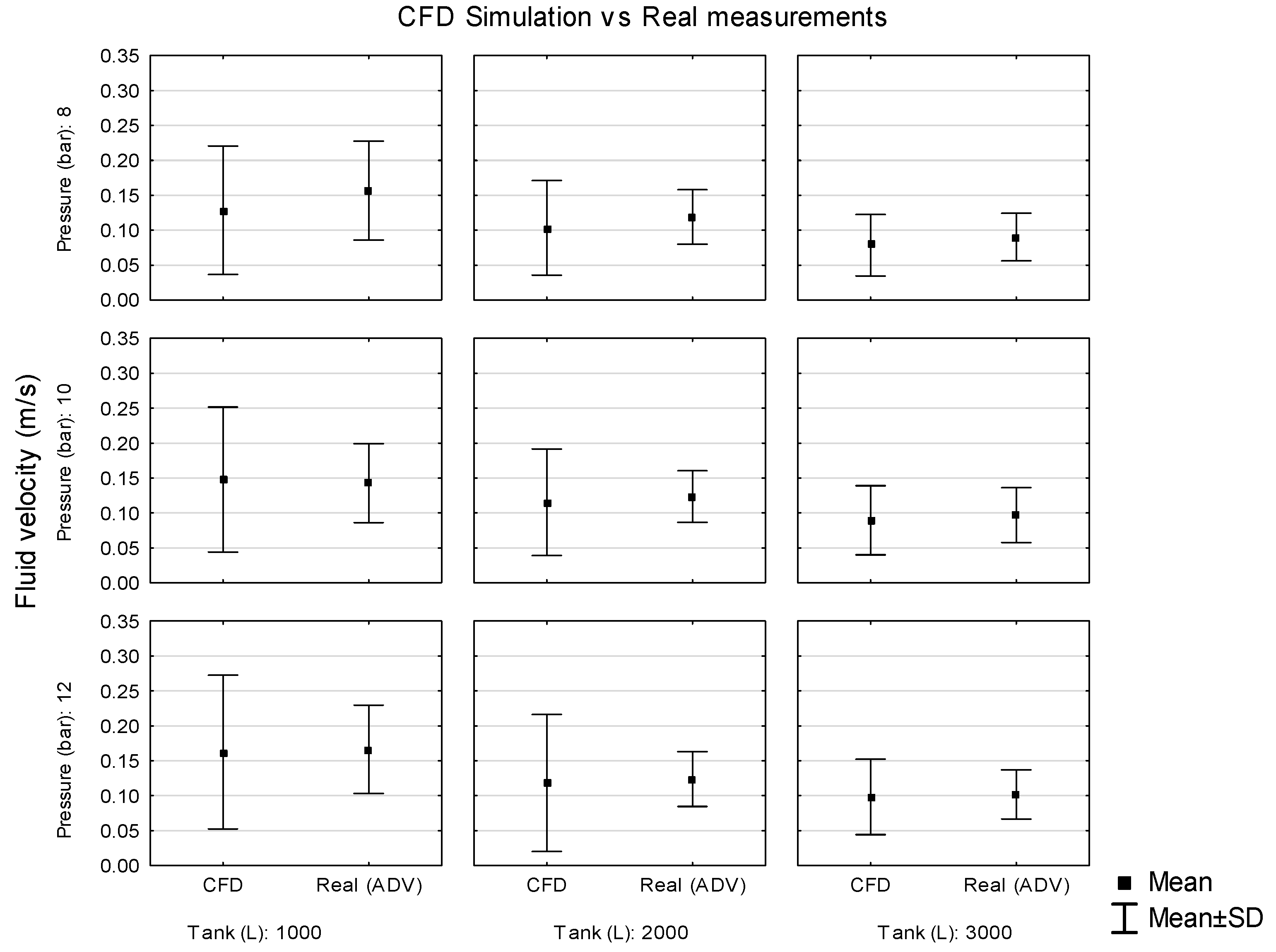
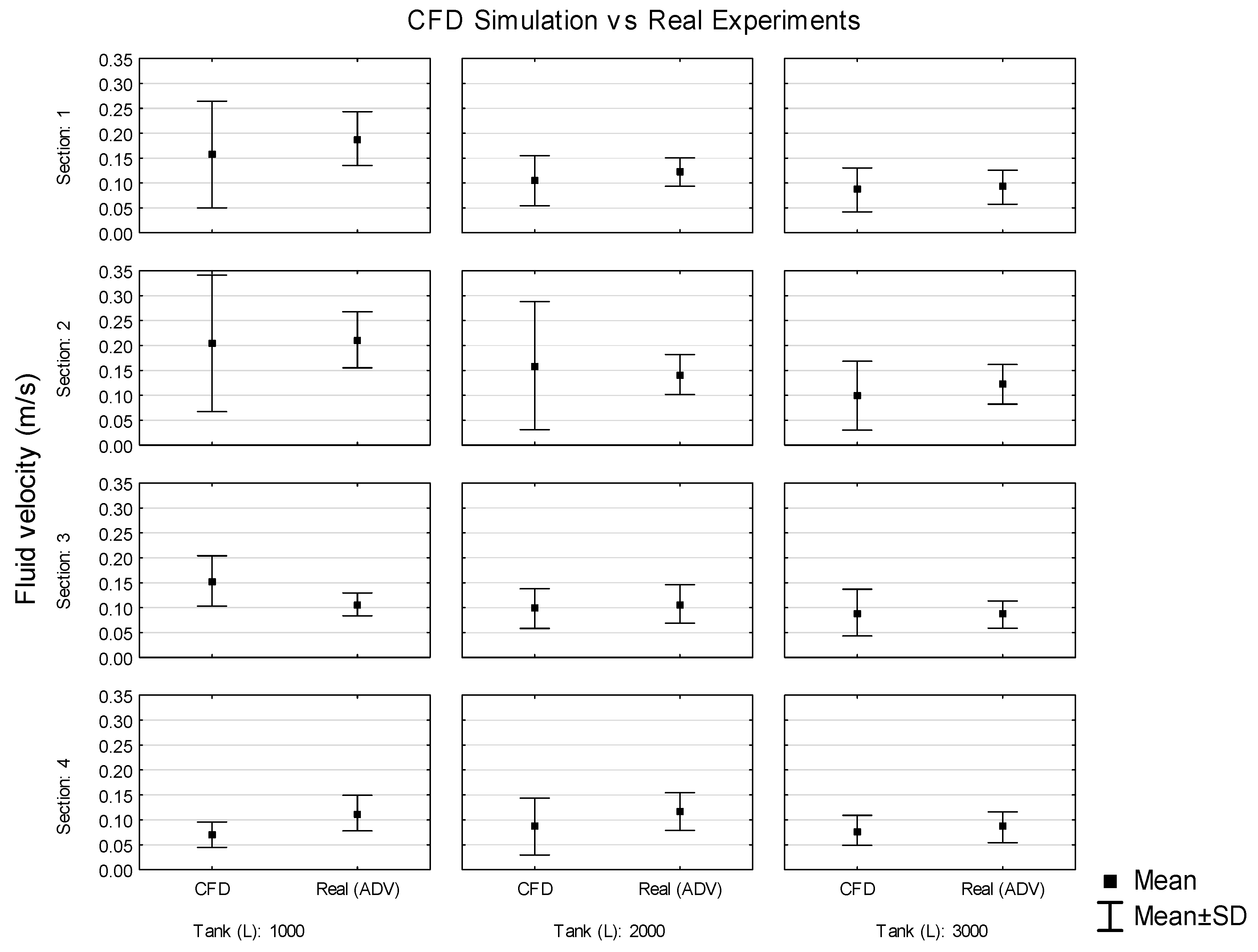
3.1. Mean CFD Velocities

In a first analysis, the mean velocities obtained with the model for a specific setting of the agitation system (pressure, water level, and number of active nozzles) were analyzed. In this way, the variability of the data is absorbed and an overall evaluation of the effect of the regulation parameters is obtained to be compared to that obtained with the experimental data.

In this way, considering the effect of the level of water inside the tank (1000, 2000, and 3000 L) and the pressure of the agitation circuit, Figure 6 shows the mean fluid velocity (points according to the level of water and the pressure). CFD results were in accordance with the experimental ones (ADV measurements) and with those obtained by [23] who used an ADV velocimeter in an aquaculture circular tank and obtained higher velocities with the lower levels of water in the tank.

The CFD simulation reasonably predicted that the most determining factor in the agitation velocity was the water level in the tank. The pressure of the agitation circuit also had a significant influence on the fluid velocity, with higher velocities generally occurring as the pressure increased. These CFD data were consistent with the experimental ones (ADV measurements) and also with those obtained by [9], who measured fluid velocity using a hot-film anemometer at nine points inside a sprayer tank of 1136 L, working with four nozzles, and registered fluid velocity increments between 40% and 130% as the system pressure increased from 2.07 to 4.70 bar.

In general, results were consistent in both CFD modeling and actual ADV measurements, with CFD values lower than those obtained with experimental measurements.

The number of active nozzles in the agitation system also significantly affected the fluid velocity (Figure 7); velocities were lower with four active nozzles than those with two nozzles. This fact reflects that the location of the nozzles within the tank can affect the fluid velocity more significantly than does the number of nozzles activated. In this case, the nozzles were located on opposite sides of the tank so the effect of increasing the number of active nozzles did not result in an increase in velocity. These results were consistent in both CFD modeling and actual ADV measurements. However, other authors [9] who worked with eight nozzles in the agitation system registered a 14.8% velocity increase compared to that for four nozzles, although, in this case, all of the nozzles were aligned in the lower part of the tank, placed on the same work plane.

This fact reinforces the importance of using CFD models to properly locate nozzles inside the tank during the design phase of the sprayer. When only two nozzles worked, they did so in opposite corners of the tank, so that there was no interaction between the liquid flow rates generated by each nozzle. However, when the four nozzles worked, they faced each other 2 to 2 (Figure 8), so the currents generated tended to be counteracted. Therefore, thanks to CFD models, it can be deduced that the location of the nozzles and the holes of the central breakwater are determining factors in the behavior of the fluid inside the tank.

If data are compared by averaging the velocities of the points belonging to the same height (Figure 9), the theoretical velocities obtained in the computer model fit quite well with the experimental ones, although at height 2 (0.65 m from the bottom), the CFD values are significantly lower than those determined experimentally. If the study is carried out by sections (Figure 10), the CFD simulation correctly predicts the section that is the one with the highest speeds in any case.

By analyzing the effect of the regulation parameters of the agitation system on the fluid velocity, and considering the mean velocities obtained as a function of the water level in the tank, the CFD models provide results similar to those obtained with experimental measurements. In this sense, it is clearly useful to use CFD models to obtain data that help in the decision making related to the regulation and design of the agitation system, thereby reducing experimental tests in the first phases of equipment development. It should be remembered that theoretical velocities calculated in the CFD simulation always had a greater variability than those obtained in the experimental tests.

3.2. Validation Error

Analyzing point by point, without grouping data according to the setting parameters of the agitation system, the relative errors (%) obtained with the model and those obtained with the experimental test have been quantified using Equation (1).

$$E=\frac{1}{N}{\displaystyle \sum \frac{\left(V_m-V_c\right)}{V_m}\times 100},$$

(1)

where “E” is the relative error (%), “V_m” is the value measured, “V_c” is the value calculated by the simulation with CFD, and “N” is the number of points measured.

According to the developed models, a total of 360 data have been compared. As shown previously, the mean velocities obtained in the real experiment were very similar to those by CFD simulation, although a higher standard deviation of the data is observed in the simulation (

Table 3. Model errors considering all measuring points.

	Real Experiment	CFD Simulations
Mean (m/s)	0.1126	0.1041
Standard deviation	0.0460	0.0723

).

However, the detailed analysis of the 360 experimental data according to Equation (1) gives an error of 45.62%. According to the usual validation criterion for this type of model [24], an error below 30% would be admissible. Data with that tolerable margin of error were obtained at 38% of the points, which would be in line with other authors [9] who have also obtained a percentage of low point-to-point correlation in similar experiments.

As an illustrative example, the correlation of the CFD model “1000 L-10 bar-4 active nozzles” with respect to the real experiment was r² = 0.002, while the mean of the velocities were 0.116 and 0.125, respectively, which, unlike the point-to-point analysis, is a fairly acceptable approximation with an error of 7%. The above case is not an exception, as in all cases (

Table 4. Relative error (%) of the mean fluid velocities estimated experimentally and by CFD, separated by calculation models.

Model	2 Active Nozzles			4 Active Nozzles
	8 Bar	10 Bar	12 Bar	8 Bar	10 Bar	12 Bar
1000	20%	12%	8%	14%	7%	14%
2000	10%	4%	12%	16%	10%	5%
3000	23%	16%	14%	3%	1%	7%

), the averages obtained with CFD are very good approximations to those measured experimentally.

An explanation for this fact would be that the CFD magnifies the results of the velocities, both up and down, so that the errors by excess are compensated with the errors by default so that the set of values does not deviate from the average by more than 30%.

4. Conclusions

CFD simulation has made it possible to estimate fluid velocities at 38% of the measuring points with relative errors of less than 30%, showing low reliability.

However, the CFD models have allowed the correct prediction of the general behavior of the fluid in the tank considering mean velocities depending on the setting parameters of the agitation system (water level in the tank, hydraulic circuit pressure, and number of active nozzles).

Analyzing the regulation parameters of the agitation system, a lower level of water in the tank or a higher pressure in the hydraulic circuit produces an increase in the velocity in the fluid, thus improving the mixing process. On the other hand, in the case of the effect of the number of active nozzles on the fluid velocity, no general relationship can be established, because the position and orientation of active nozzles are more important than their number. In this sense, CFD analysis makes it possible to detect design errors in the arrangement of the nozzles prior to machine manufacturing. Therefore, with the methodology employed, the CFD can be converted into a useful design tool, allowing decisions to be made regarding the design of the agitation system prior to the manufacture of the first prototype and also to estimate the correct setting of the agitation system.

References

1. ISO. Equipment for Crop Protection—Spraying Equipment–Part 2: Test Methods for Hydraulic Sprayers; ISO 5682-2; International Organization for Standadization: Geneva, Switerlrand, 1997. [Google Scholar]
2. Balsari, P.; Tamagnone, M.; Allochis, D.; Marucco, P.; Bozzer, C. Sprayer tank agitation check: A proposal for a simple instrumental evaluation. In Proceedings of the Fourth European Workshop on Standardised procedure for the Inspection of Sprayers -SPISE 4-, Lana, Italy, 27–29 March 2012. [Google Scholar]
3. Ozkan, H.E.; Ackerman, K.K. Instrumentation for measuring mixture variability in sprayer tanks. Appl. Eng. Agric. 1999, 15, 19–24. [Google Scholar] [CrossRef]
4. Ucar, T.; Ozkan, H.E.; Fox, R.D.; Brazee, R.D.; Derksen, R.C. Experimental study of jet agitation effects on agrochemical mixing in sprayer tanks. J. Agric. Eng. Res. 2000, 78, 195–207. [Google Scholar] [CrossRef]
5. Vondricka, J.; Schulze, P. Measurement of mixture homogeneity in direct injectionssystems. Trans. ASABE 2009, 52, 61–66. [Google Scholar] [CrossRef]
6. Tamagnone, M.; Balsari, P.; Bozzer, C.; Marucco, P. Assesment of parameters needed to design agitation systems for sprayer tanks. Asp. Appl. Biol. 2012, 114, 167–174. [Google Scholar]
7. García-Ramos, F.J.; Badules, J.; Bone, A.; Gil, E.; Aguirre, J.; Vidal, M. Application of an acoustic Doppler velocimeter to analyse the performance of the hydraulic agitation system of an agricultural sprayer. Sensors 2018, 18, 3715. [Google Scholar]
8. Armenante, P.M.; Luo, C.; Chou, C.; Fort, I.; Medek, J. Velocity profiles in a closed unbaffled vessel: Comparison between experimental LDV data and numerical CFD predictions. Chem. Eng. Sci. 1997, 52, 3483–3492. [Google Scholar] [CrossRef]
9. Ucar, T.; Fox, R.D.; Ozkan, H.E.; Brazee, R.D. Simulation of jet agitation in sprayer tanks: Comparison of predicted and measured water velocities. Trans. ASAE 2001, 44, 223–230. [Google Scholar] [CrossRef]
10. Chen, M.; Ñiao, B.; Pan, J.; Li, Q.; Gao, C. Improvement of the flow rate distribution in quench tank by measurement and computer simulation. Mater. Lett. 2006, 60, 1659–1664. [Google Scholar] [CrossRef]
11. Micheli, G.B.; Padilha, A.; Scalon, V.L. Numerical and experimental analysis of pesticide spray mixing in spray tanks. Eng. Agric. Jaboticaabal. 2015, 35, 1065–1078. [Google Scholar]
12. Xiongkuy, H.; Kleisinger, S.; Luoluo, W.; Bingli, L. Influences of dynamic factors and filling level of spray in the tank on the efficacy of hydraulic agitation of the sprayer. Trans. Chin. Soc. Agric. Eng. 1999, 15, 131–134. [Google Scholar]
13. García, C.M.; Cantero, M.I.; Niño, Y.; García, M.H. Turbulence measurements with acoustic Doppler velocimeters. J. Hydraul. Eng. 2005, 131, 1062–1073. [Google Scholar] [CrossRef]
14. Poindexter, C.M.; Rusello, P.J.; Variano, E.J. Acoustic Doppler velocimeter-induced acoustic streaming and its implication for measurement. Exp. Fluids 2011, 50, 1429–1442. [Google Scholar] [CrossRef]
15. MacVicar, B.J.; Beaulieu, E.; Champagne, V.; Roy, A.G. Measuring water velocity in highly turbulent flows: Field tests of an electromagnetic current meter (ECM) and an acoustic Doppler velocimeter (ADV). Earth Surf. Process. Landf. 2007, 32, 1412–1432. [Google Scholar] [CrossRef]
16. Hosseini, S.A.; Shamsai, A.; Ataie-Ashtiani, B. Synchronous measurements of the velocity and concentration in low density turbidity currents using an acoustic Doppler velocimeter. Flow Meas. Instrum. 2006, 17, 59–68. [Google Scholar] [CrossRef]
17. Sharma, A.; Maddirala, A.K.; Kumar, B. Modified singular spectrum analysis for despiking acoustic Doppler velocimeter (ADV) data. Measurement 2018, 117, 339–346. [Google Scholar] [CrossRef]
18. Baker, T. Mesh generation: Art of Science? Prog. Aerosp. Sci. 2005, 41, 29–63. [Google Scholar] [CrossRef]
19. Tamburini, A.; Cipollina, A.; Micale, G.; Brucato, A.; Ciofalo, M. CFD prediction of solid particle distribution in baffled stirred vessels under partial to complete suspension conditions. AIDIC Conf. Ser. 2013, 11, 391–400. [Google Scholar] [CrossRef]
20. Akiti, O.; Armenante, P.M. Experimentally-Validated Micromixing-Based CFD Model for Fed-Batch Stirred-Tank Reactors. AIChE J. 2004, 50, 566–577. [Google Scholar] [CrossRef]
21. Deglon, D.A.; Meyer, C.J. CFD modelling of stirred tanks: Numerical considerations. Miner. Eng. 2006, 19, 1059–1068. [Google Scholar] [CrossRef]
22. Wasewar, K.L.; Sarathi, J.V. CFD modelling and simulation of jet mixed tanks. Eng. Appl. Comput. Fluid Mech. 2008, 2, 155–171. [Google Scholar] [CrossRef] [Green Version]
23. Oca, J.; Masalo, I. Flow pattern in aquaculture circular tanks: Influence of flow rate, water depth, and water inlet & outlet features. Aquacult. Eng. 2013, 52, 65–72. [Google Scholar]
24. Delele, M.A. Engineering Design of Spraying Systems for Horticultural Applications Using Computational Fluid Dynamics. Ph.D. Thesis, Leuven Catholic University, Leuven, Belgium, 2009. [Google Scholar]
Figure 1. Geometry of the sprayer tank with a 3000 L capacity. (a) Exterior 3D view; (b) longitudinal interior 2D view. Dimensions in millimeters.
Agronomy 09 00769 g001
Figure 2. (a) Left. Cross-sections of velocity measurement points inside the tank (dimensions in millimeters); (b) Right. Velocity measurement points within each of the four sections.
Agronomy 09 00769 g002
Figure 3. 3D view of 3 mesh configurations of the sprayer tank for 1000 (left), 2000 (center), and 3000 L (right) of water inside.
Agronomy 09 00769 g003
Figure 4. Contours of y+ in the tank with (left) 3000 and (right) 1000 L, with two nozzles in use and 10 bar pressure.
Agronomy 09 00769 g004
Figure 5. Liquid velocity for a 1000 L model obtained at 8 sampling points as the iterations were in progress. In this case, it can be concluded that 1500 iterations were sufficient to consider the model as stabilized.
Agronomy 09 00769 g005
Figure 6. Mean fluid velocities, estimated by CFD and experimentally measured, according to the level of water in the tank and pressures of the nozzle circuits.
Agronomy 09 00769 g006
Figure 7. Mean fluid velocities, estimated by CFD and experimentally measured, according to the number of active nozzles.
Agronomy 09 00769 g007
Figure 8. Iso-velocity diagram at 0.2 m/s with (left) two and (right) four active nozzles in a tank with 1000 L. Scale 1:60.
Agronomy 09 00769 g008
Figure 9. Mean fluid velocities, estimated by CFD and experimentally measured, according to the height of the measurement point (1: 0.37 m; 2: 0.65 m, 3: 0.93 m).
Agronomy 09 00769 g009
Figure 10. Mean fluid velocities, estimated by CFD and experimentally measured, according to the section of the measurement point.
Agronomy 09 00769 g010