Managing Tallgrass Prairies for Productivity and Ecological Function: A Long-Term Grazing Experiment in the Southern Great Plains, USA

 ,
,  ,
,
Abstract
:1. Introduction
2. Stakeholder Engagement
3. Research Questions
4. Site Description
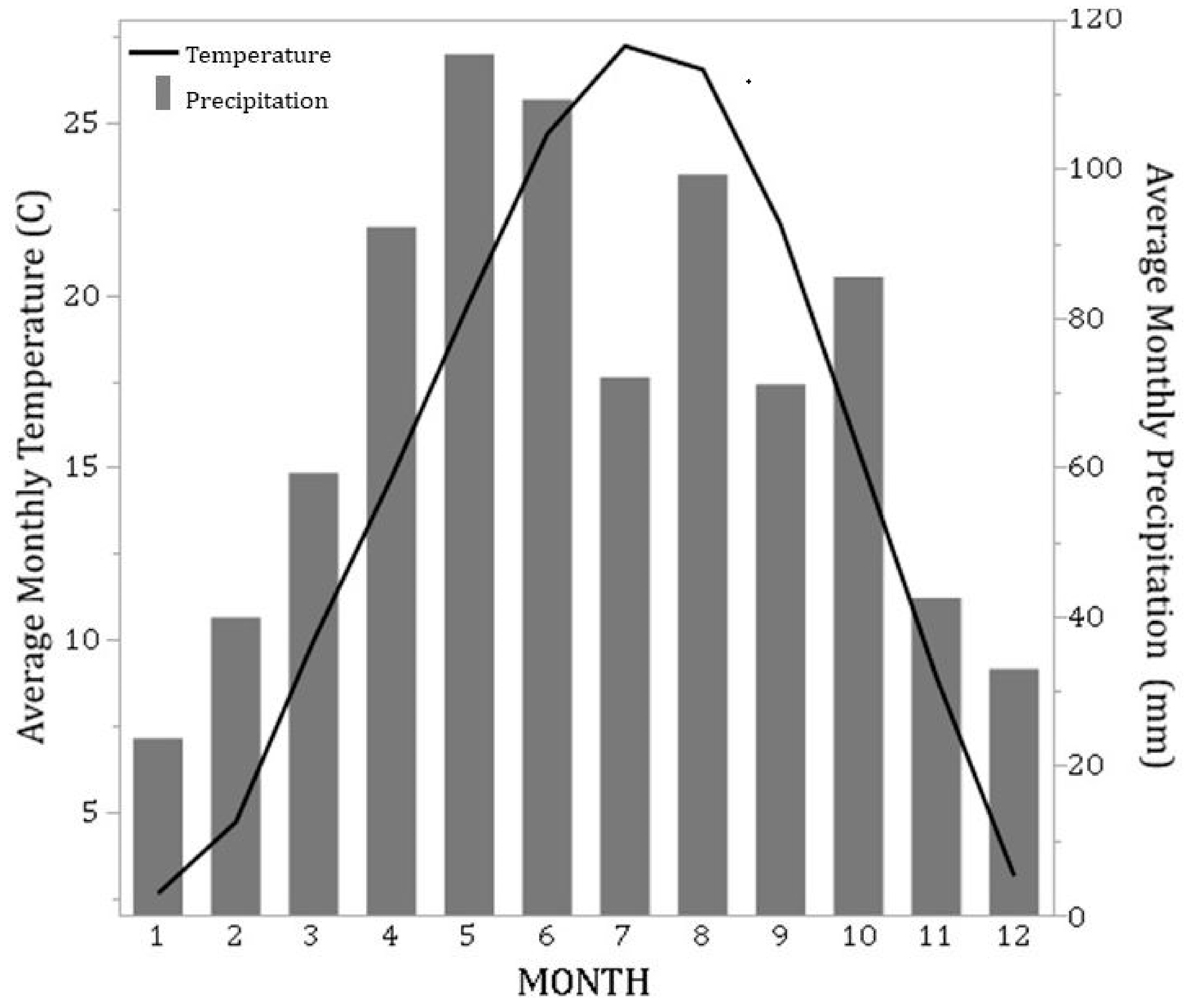
4.1. Climate
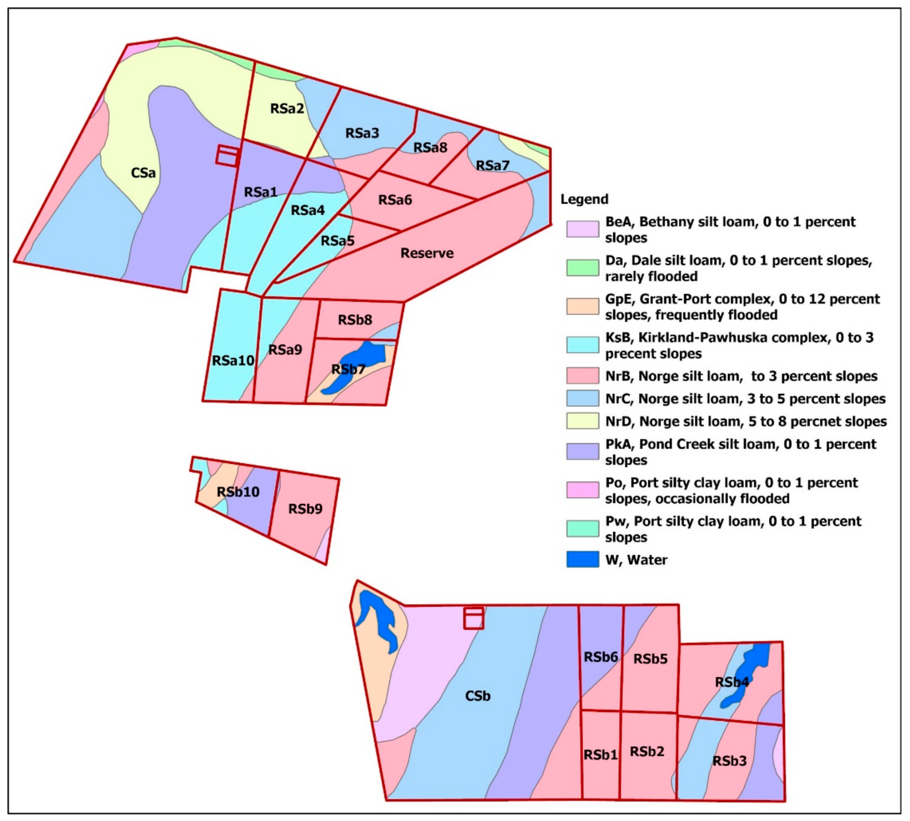
4.2. Soils and Vegetation
4.3. Layout and Experimental Design
5. Materials and Methods
5.1. Soil Parameters
5.2. Forage Biomass and Nutritive Parameters
5.3. Animal Parameters
5.4. Statistical Analysis
6. Results
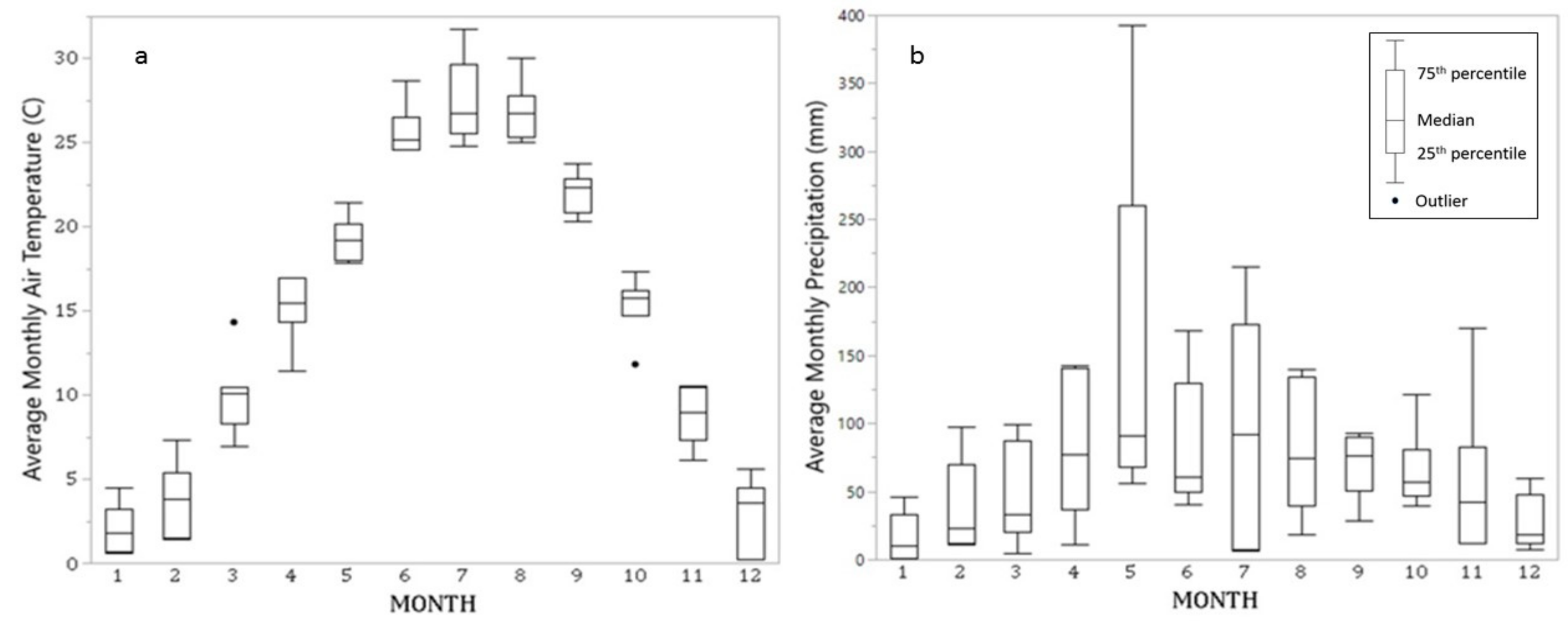
6.1. Temperature and Precipitation
6.2. Soil parameters
Soil Bulk Density
6.3. Forage
6.3.1. Above-Ground Biomass
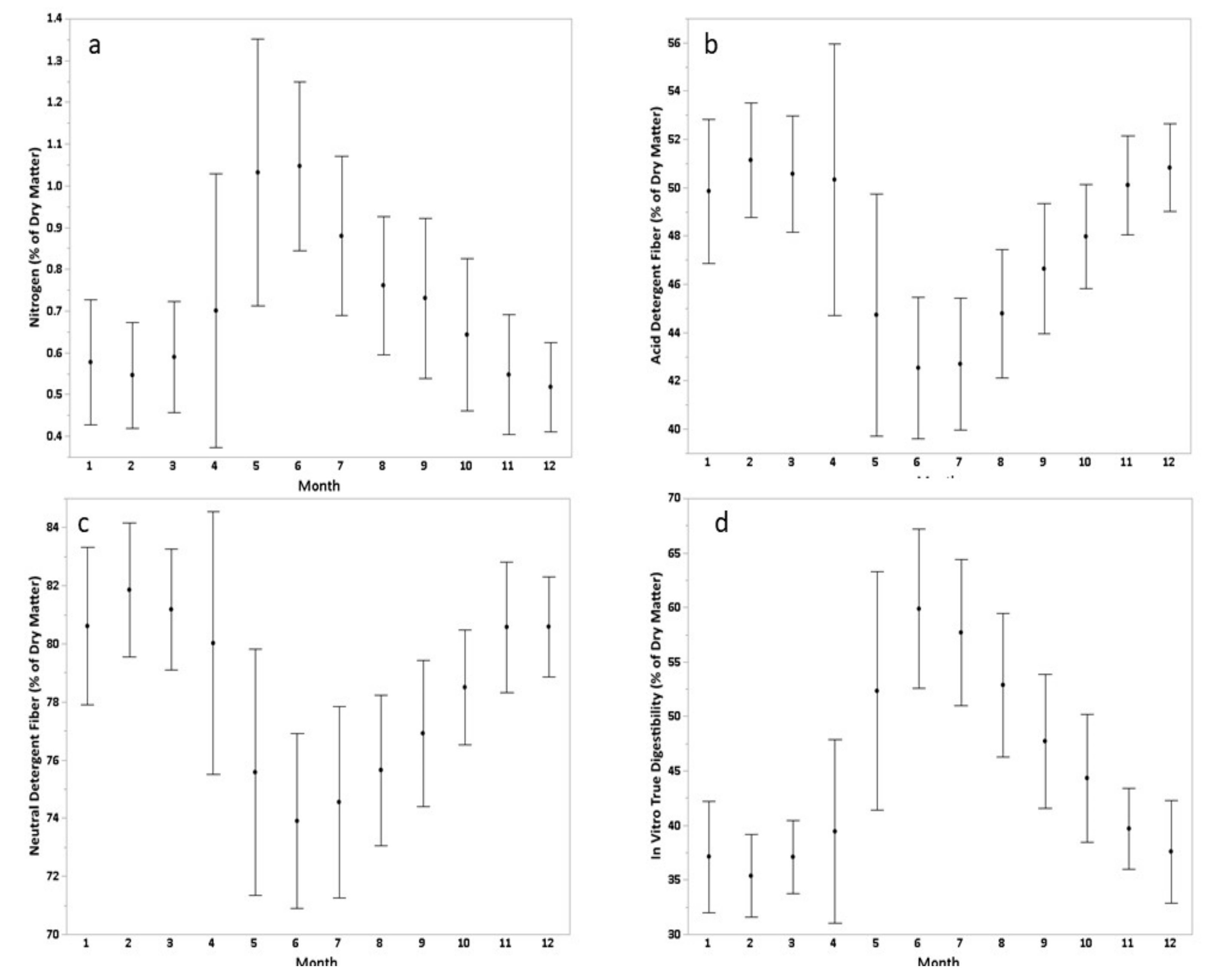
6.3.2. Monthly Mean and Variability of Forage Nutritive Values
6.3.3. Forage Nutritive Values during Summer Grazing Season
6.4. Animal Parameters
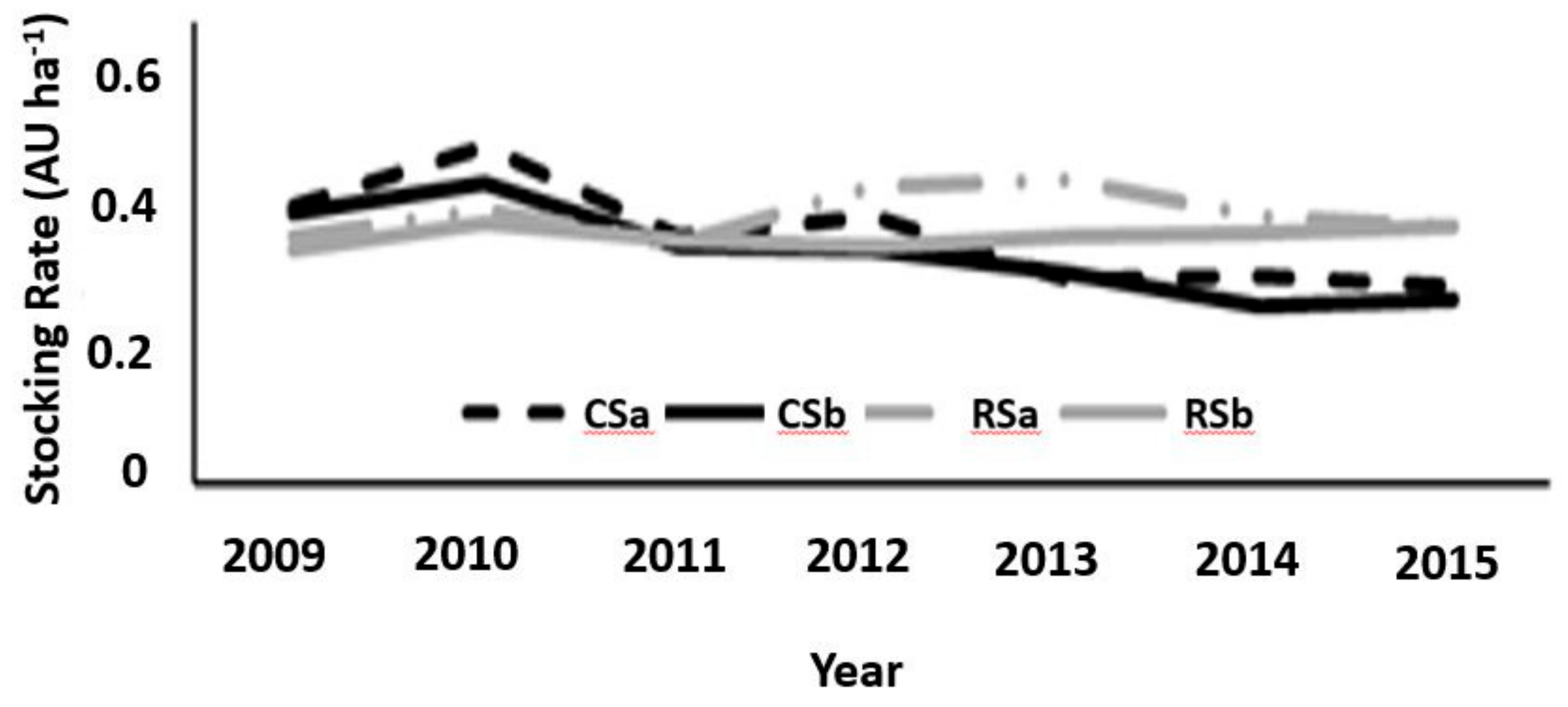
6.4.1. Stocking Rate
6.4.2. Animal Performance
7. Discussion
8. Conclusions
Author Contributions
Funding
Acknowledgments
Conflicts of Interest
Disclaimer
Appendix A
Appendix A.1. High-Density, Short-Duration (HDSD) Treatments
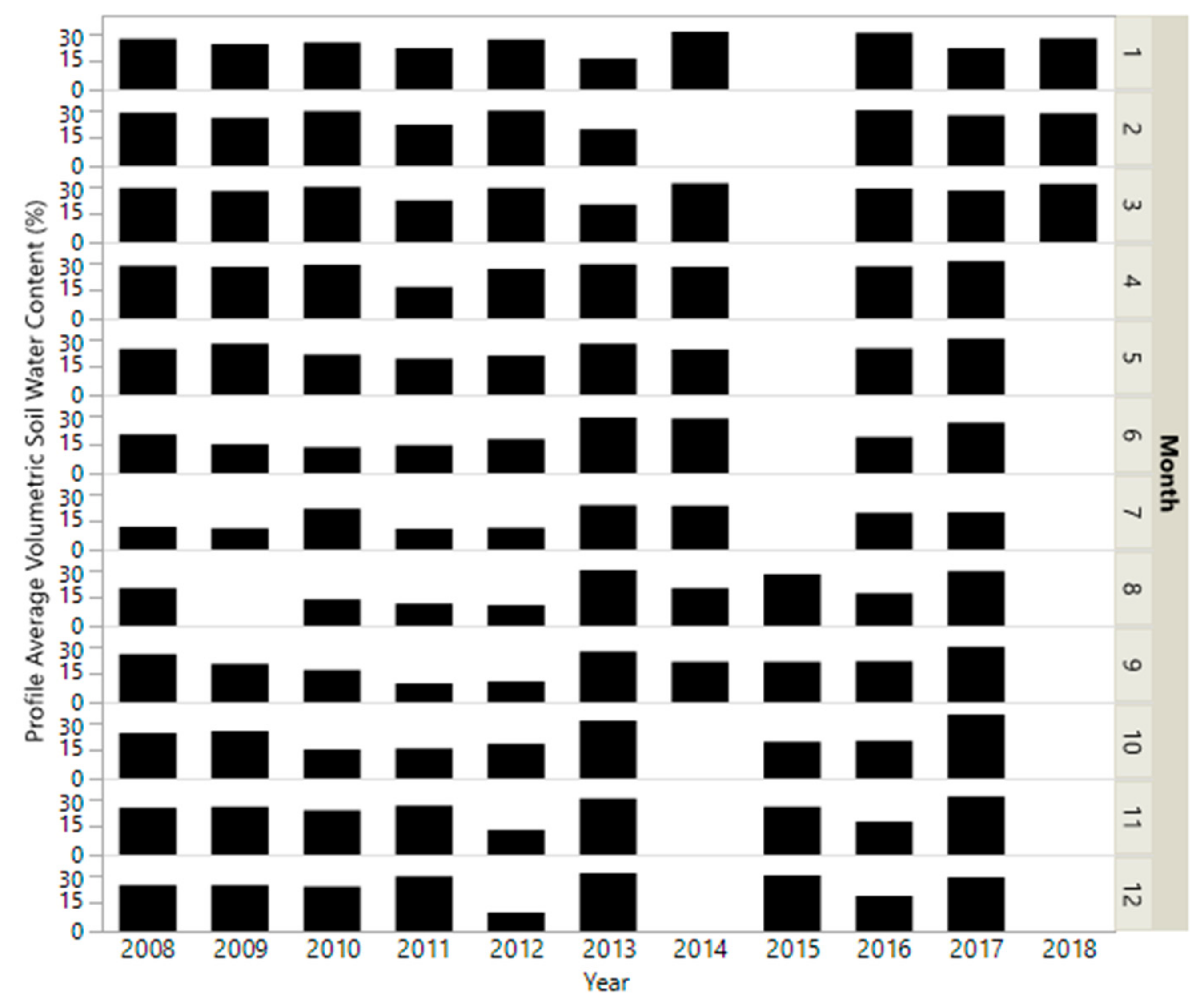
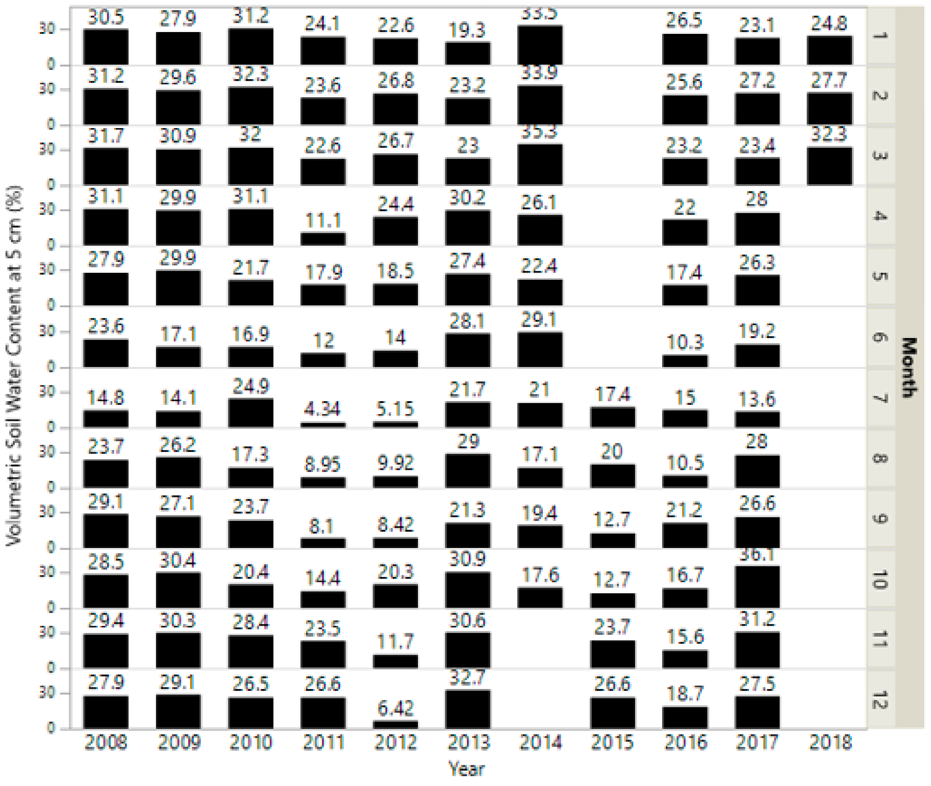
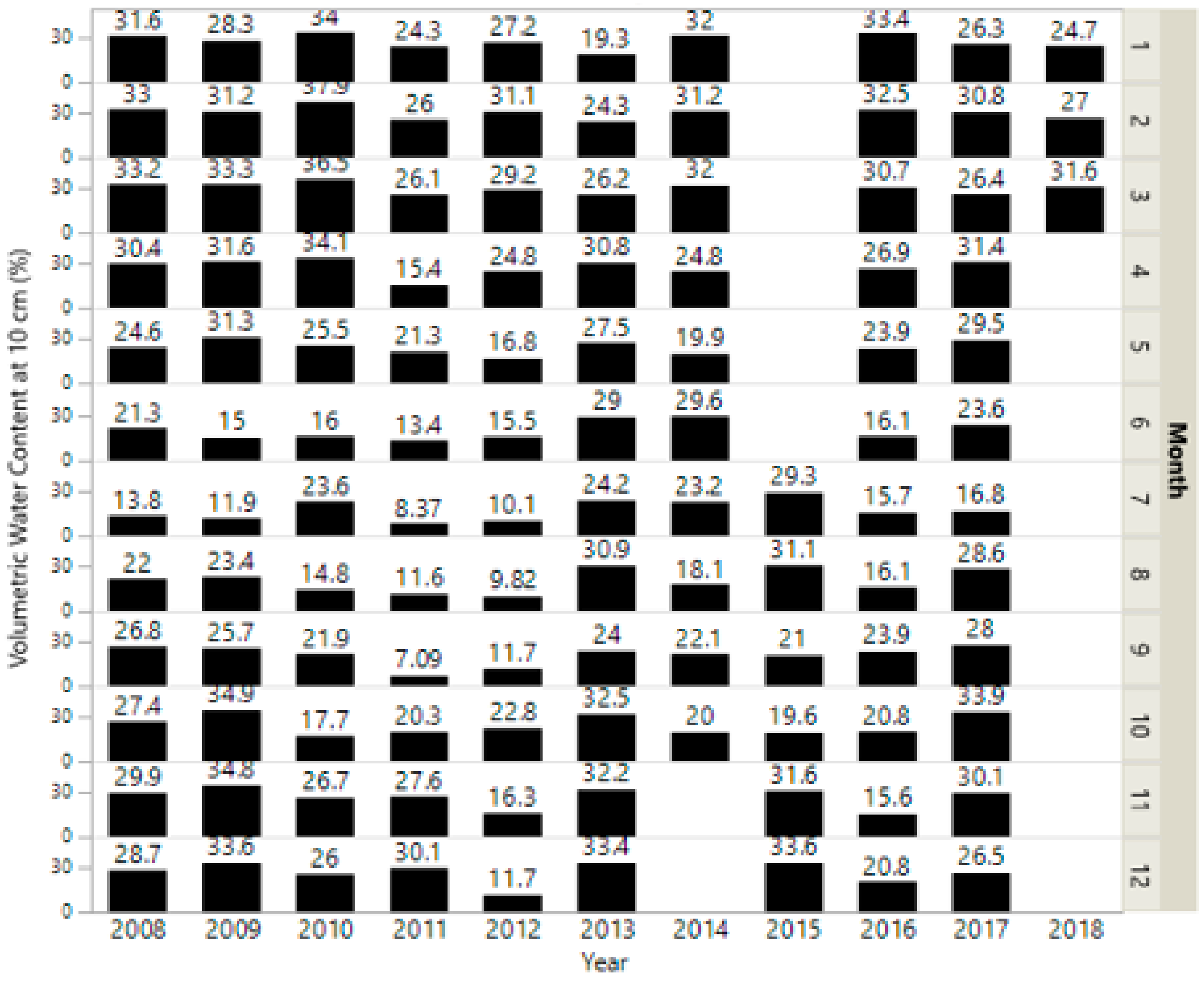
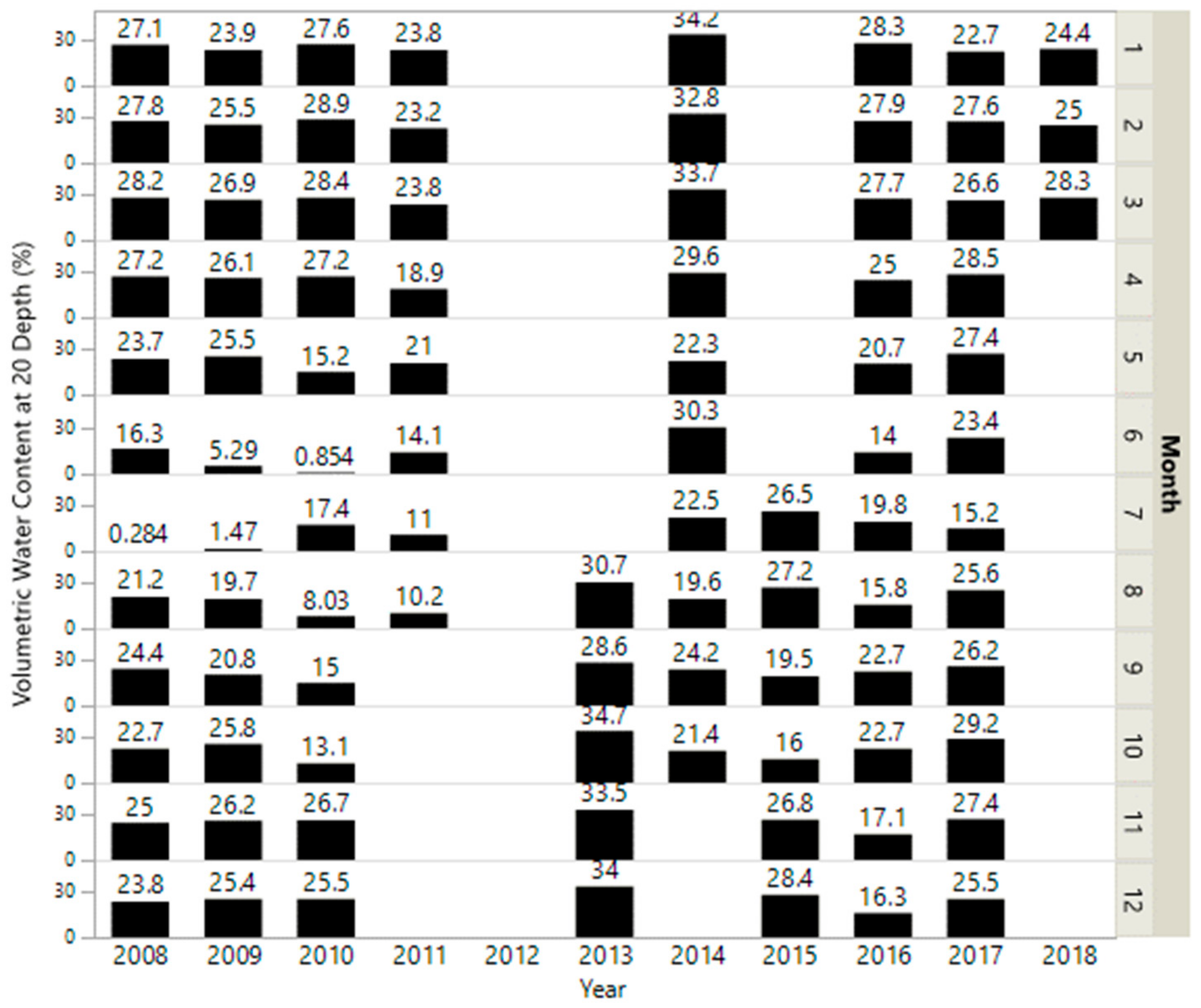
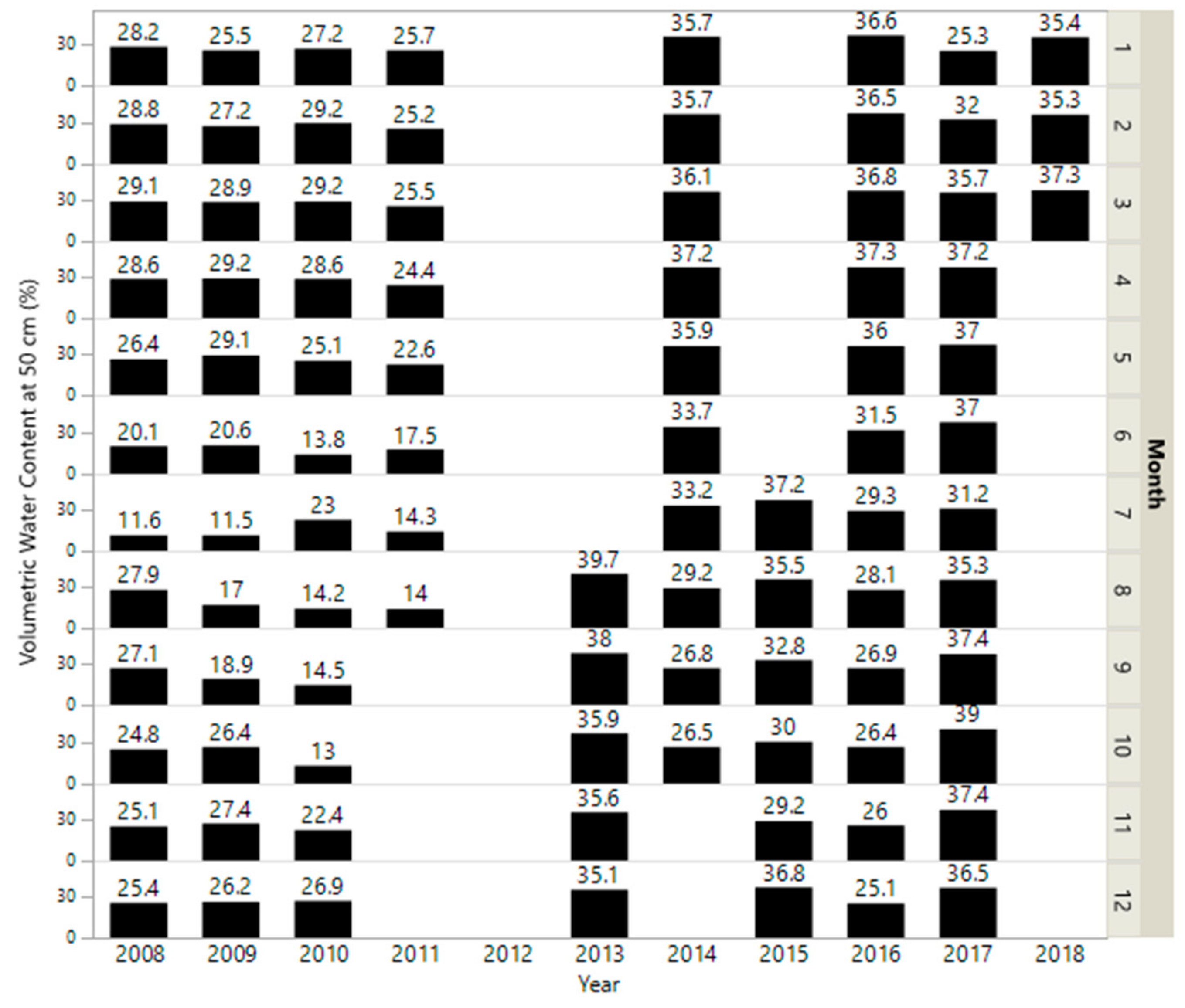
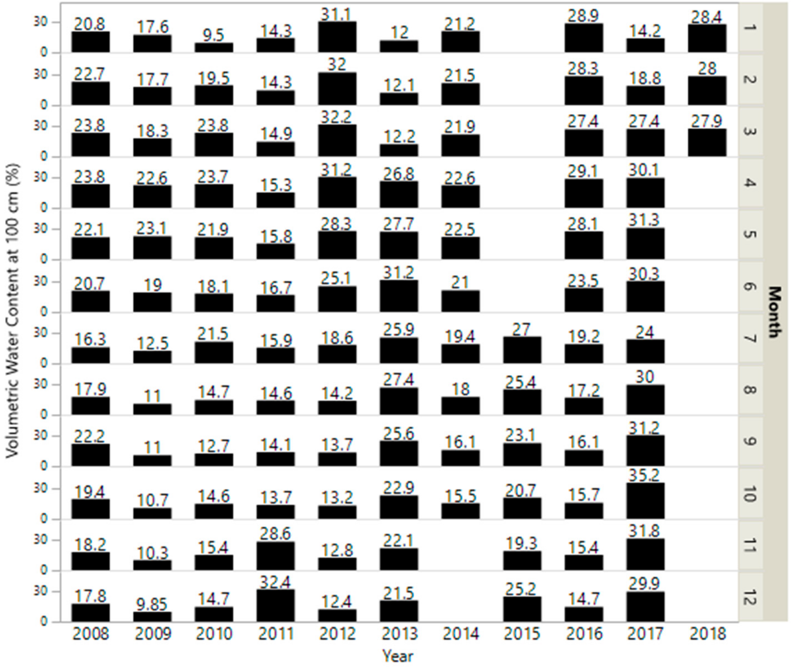
Appendix A.2. Soil Water Content by Depth


Appendix A.3. Soil Properties

| Treatment † | % Sand | % Clay | pH | EC (uS cm−1) | ||
|---|---|---|---|---|---|---|
| 0–30 cm | 0–15 cm | 15–30 cm | 0–15 cm | 15–30 cm | ||
| CS | 26.7 A | 23.1 A | 6.1 A | 5.92 A | 329.8 A | 260.0 A |
| RS | 22.6 A | 25.3 A | 6.1 A | 6.02 A | 292.8 A | 207.5 A |
| Year, Treatment † | Depth Interval | |
|---|---|---|
| 0–15 cm | 15–30 cm | |
| ----------- g cm−3--------- | ||
| 2009, CS | 1.04 C | 1.21 B |
| 2009, RS | 1.12 B | 1.21 B |
| 2012, CS | 1.28 A | 1.35 A |
| 2012, RS | 1.28 A | 1.33 A |
| 2017, CS | 1.05 C | 1.14 C |
| 2017, RS | 1.07 BC | 1.16 C |
References
- Bigelow, D.P.; Borchers, A. Major Uses of Land in the United States, 2012; EIB-178; United States Department of Agriculture: Economic Research Service: Washington, DC, USA, 2018. [Google Scholar]
- Steiner, J.L.; Franzluebbers, A.J.; Neely, C.; Ellis, T.; Aynekulu, E. Enhancing soil and landscape quality in smallholder grazing systems. In Soil Management of Smallholder Agriculture. Advances in Soil Science; Lal, R., Ed.; CRC Press: Boca Raton, FL, USA, 2014; pp. 63–111. [Google Scholar]
- Panunzi, E. Are Grasslands under Threat? Brief Analysis of FAO Statistical Data on Pasture and Fodder Crops; UN Food and Agriculture Organization: Rome, Italy, 2008. [Google Scholar]
- Neely, C.; Bunning, S.; Wilkes, A. Review of Evidence on Drylands Pastoral Systems and Climate Change; Land and Water Discussion Paper No. 8; Food and Agriculture Organization of the United Nations: Rome, Italy, 2009. [Google Scholar]
- Smith, M.R.; Myers, S.S. Impact of anthropogenic CO2 emissions on global human nutrition. Nat. Clim. Chang. 2018, 8, 834–839. [Google Scholar] [CrossRef]
- Brussaard, L.; Caron, P.; Campbell, B.; Lipper, L.; Mainka, S.; Rabbinge, R.; Babin, D.; Pulleman, M. Reconciling biodiversity conservation and food security: Scientific challenges for a new agriculture. Curr. Opin. Environ. Sustain. 2010, 2, 34–42. [Google Scholar] [CrossRef]
- Sollenberger, L.E.; Kohmann, M.M.; Dubeux, J.C.B., Jr.; Silveira, M.L. Grassland management affects delivery of regulating and supporting ecosystem services. Crop Sci. 2019, 59, 441–459. [Google Scholar] [CrossRef]
- Boone, R.B.; Conant, R.T.; Sircely, J.; Thornton, P.K.; Herrero, M. Climate change impacts on selected global rangeland ecosystem services. Glob. Chang. Biol. 2018, 24, 1382–1393. [Google Scholar] [CrossRef]
- Hatfield, J.L.; Boote, K.J.; Kimball, B.A.; Ziska, L.H.; Izaurralde, R.C.; Ort, D.; Thomson, A.M.; Wolfe, D. Climate impacts on agriculture: Implications for crop production. Agron. J. 2011, 103, 351–370. [Google Scholar] [CrossRef]
- Izaurralde, R.C.; Thomson, A.M.; Morgan, J.A.; Fay, P.A.; Polley, H.W.; Hatfield, J.L. Climate impacts on agriculture: Implications for forage and rangeland production. Agron. J. 2011, 103, 371–381. [Google Scholar] [CrossRef]
- Steiner, J.L.; Wagle, P.; Gowda, P. Management of water resources for grasslands. In Improving Grassland and Pasture Management in Agriculture; Marshall, A., Collins, R., Eds.; Burleigh Dodds Science Publishing: Cambridge, UK, 2017; pp. 265–282. [Google Scholar]
- Samson, F.B.; Knopf, F.L.; Ostlie, W.R. Great Plains ecosystems: Past, present, and future. Wildl. Soc. Bull. 2004, 32, 6–15. [Google Scholar] [CrossRef]
- Samson, F.; Knopf, F. Prairie conservation in North America. BioScience 1994, 44, 418–421. [Google Scholar] [CrossRef]
- Conner, R.; Seidl, A.; VanTassell, L.; Wilkins, N. United States Grasslands and Related Resources: An Economic and Biological Trends Assessment. 2002. Available online: http://twri.tamu.edu/media/256592/unitedstatesgrasslands.pdf (accessed on 25 March 2019).
- Askins, R.; Chavez-Ramirez, F.; Dale, B.; Haas, C.; Herkert, J.; Knopf, F.; Vickery, P.D. Conservation of Grassland Birds in North America: Understanding Ecological Processes in Different Regions; The American Ornithologists’ Union: Chicago, IL, USA, 2007; pp. 1–46. [Google Scholar]
- Comer, P.J.; Hak, J.C.; Kindscher, K.; Muldavin, E.; Singhurst, J. Continent-scale landscape conservation design for temperate grasslands of the Great Plains and Chihuahuan Desert. Nat. Areas J. 2018, 38, 196–211. [Google Scholar] [CrossRef]
- Hill, J.M.; Egan, J.F.; Stauffer, G.E.; Diefenbach, D.R. Habitat availability is a more plausible explanation than insecticide acute toxicity for US grassland bird species declines. PLoS ONE 2014, 9, e98064. [Google Scholar] [CrossRef]
- Derner, J.D.; Smart, A.J.; Toombs, T.P.; Larsen, D.; McCulley, R.L.; Goodwin, J.; Sims, S.; Roche, L.M. Soil health as a transformation change agent for US grazinglands management. Rangel. Ecol. Manag. 2018, 71, 403–408. [Google Scholar] [CrossRef]
- Sarkar, S. Phenology and carbon fixing: A satellite-based study over Continental USA. Int. J. Remote Sens. 2018, 39, 1–16. [Google Scholar] [CrossRef]
- Teague, W.R. Toward restoration of ecosystem function and livelihoods on grazed agroecosystems. Crop Sci. 2015, 55, 2550–2556. [Google Scholar] [CrossRef]
- Park, J.-Y.; Ale, S.; Teague, W.R. Simulated water quality effects of alternate grazing management practices at the ranch and watershed scales. Ecol. Model. 2017, 360, 1–13. [Google Scholar] [CrossRef]
- Wang, J.; Xiao, X.; Qin, Y.; Doughty, R.B.; Dong, J.; Zou, Z. Characterizing the encroachment of juniper forests into sub-humid and semi-arid prairies from 1984 to 2010 using PALSAR and Landsat data. Remote Sens. Environ. 2018, 205, 166–179. [Google Scholar] [CrossRef]
- Caterina, G.L.; Will, R.E.; Turton, D.J.; Wilson, D.S.; Zou, C.B. Water use of Juniperus virginiana trees encroached into mesic prairies in Oklahoma, USA. Ecohydrology 2014, 7, 1124–1134. [Google Scholar]
- Qiao, L.; Zou, C.B.; Stebler, E.; Will, R.E. Woody plant encroachment reduces annual runoff and shifts runoff mechanisms in the tallgrass prairie, USA. Water Resour. Res. 2017, 53, 4838–4849. [Google Scholar] [CrossRef]
- Acharya, B.S.; Hao, Y.; Ochsner, T.E.; Zou, C.B. Woody plant encroachment alters soil hydrological properties and reduces downward flux of water in tallgrass prairie. Plant Soil 2017, 414, 379–391. [Google Scholar] [CrossRef]
- Zhou, Y.; Xiao, X.; Zhang, G.; Wagle, P.; Bajgain, R.; Dong, J.; Jin, C.; Basara, J.B.; Anderson, M.C.; Hain, C.; et al. Quantifying agricultural drought in tallgrass prairie region in the U.S. Southern Great Plains through analysis of a water-related vegetation index from MODIS images. Agric. For. Meteorol. 2017, 246, 111–122. [Google Scholar] [CrossRef]
- Augustine, D.J.; Blumenthal, D.M.; Springer, T.L.; LeCain, D.R.; Gunter, S.A.; Derner, J.D. Elevated CO2 induces substantial and persistent declines in forage quality irrespective of warming in mixed grass prairie. Ecol. Appl. 2018, 28, 721–735. [Google Scholar] [CrossRef]
- Riitters, K.H.; Wickham, J.D. How far to the nearest road? Front. Ecol. Environ. 2003, 1, 125–129. [Google Scholar] [CrossRef]
- Lal, R. Global food security and nexus thinking. J. Soil Water Conserv. 2016, 71, 85A–90A. [Google Scholar] [CrossRef]
- Holechek, J.L.; Pieper, R.D.; Herbel, C.H. Range Management Principles and Practices; Chapter 8 Considerations Concerning Stocking Rate; Pearson, Prentice Hall: Upper Saddle River, NJ, USA, 2004; pp. 216–260. [Google Scholar]
- Savory, A.; Butterfield, J. Holistic Management: A New Framework for Decision Making, 2nd ed.; Island Press: Washington, DC, USA, 1999; 644p. [Google Scholar]
- Teague, W.R.; Apfelbaum, S.; Lall, R.; Kreuter, U.P.; Rowntree, J.; Davies, C.A.; Concer, R.; Rasmussen, M.; Hatield, J.; Wang, T.; et al. The role of ruminants in reducing agriculture’s carbon footprint in North America. J. Soil Water Conserv. 2016, 71, 156–164. [Google Scholar] [CrossRef]
- Briske, D.D.; Derner, J.D.; Brown, J.R.; Fuhlendorf, S.D.; Teague, W.R.; Havstad, K.M.; Gillen, R.L.; Ash, A.J.; Willms, W.D. Rotational grazing on rangelands: Reconciliation of perception and experimental evidence. Rangel. Ecol. Manag. 2008, 61, 3–17. [Google Scholar] [CrossRef]
- Briske, D.D.; Sayre, N.F.; Huntsinger, L.; Fernandez-Gimenez, M.; Budd, B.; Derner, J.D. Origin, persistence, and resolution of the rotational grazing debate: Integrating human dimension into rangeland research. Rangel. Ecol. Manag. 2011, 64, 325–334. [Google Scholar] [CrossRef]
- Derner, J.; Briske, D.; Boutton, T. Does grazing mediate soil carbon and nitrogen accumulation beneath C4, perennial grasses along an environmental gradient? Plant Soil 1997, 191, 147–156. [Google Scholar] [CrossRef]
- Fuhlendorf, S.D.; Zhang, H.; Tunnell, T.; Engle, D.M.; Cross, A.F. Effects of grazing on restoration of southern mixed prairie soils. Restor. Ecol. 2002, 10, 401–407. [Google Scholar] [CrossRef]
- Henderson, D.C.; Ellert, B.H.; Naeth, M.A. Grazing and soil carbon along a gradient of Alberta rangelands. J. Range Manag. 2004, 57, 402–410. [Google Scholar] [CrossRef]
- Owensby, C.E.; Ham, J.M.; Auen, L.M. Fluxes of CO2 from grazed and ungrazed tallgrass prairie. Rangel. Ecol. Manag. 2006, 59, 111–127. [Google Scholar] [CrossRef]
- Follett, R.F.; Reed, D.A. Soil carbon sequestration in grazing lands: Societal benefits and policy implications. Rangel. Ecol. Manag. 2010, 63, 4–15. [Google Scholar] [CrossRef]
- Northup, B.K.; Daniel, J.A. Distribution of soil bulk density and organic matter along an elevation gradient in central Oklahoma. Trans. ASABE 2010, 53, 1749–1757. [Google Scholar] [CrossRef]
- Franzluebbers, A.; Stuedemann, J. Bermudagrass management in the Southern Piedmont USA: VII. Soil-profile organic carbon and total nitrogen. Soil Sci. Soc. Am. J. 2005, 69, 1455–1462. [Google Scholar] [CrossRef]
- Northup, B.K.; Starks, P.J.; Turner, K.E. Stocking methods and soil macronutrient distributions in southern tallgrass paddocks: Are there linkages? Agronomy 2019, 9, 281. [Google Scholar] [CrossRef]
- Northup, B.K.; Starks, P.J.; Turner, K.E. Soil macronutrient responses in diverse landscapes of southern tallgrass to two stocking methods. Agronomy 2019, 9, 329. [Google Scholar] [CrossRef]
- Starks, P.J.; Steiner, J.L.; Neel, J.P.S.; Turner, K.E.; Northup, B.K.; Gowda, P.H.; Brown, M.A. Assessment of the standardized precipitation and evaporation index (SPEI) as a potential management tool for grasslands. Agronomy 2019, 9, 235. [Google Scholar] [CrossRef]
- Spiegal, S.; Bestelmeyer, B.T.; Archer, D.W.; Augustine, D.J.; Boughton, E.H.; Boughton, R.K.; Cavigelli, M.A.; Clark, P.E.; Derner, J.D.; Duncan, E.W.; et al. Evaluating strategies for sustainable intensification of US agriculture through the Long-Term Agroecosystem Research network. Environ. Res. Lett. 2018, 13, 034031. [Google Scholar] [CrossRef]
- Kleinman, P.J.A.; Spiegal, S.; Rigby, J.R.; Goslee, S.C.; Baker, J.M.; Bestelmeyer, B.T.; Boughton, R.K.; Bryant, R.B.; Cavigelli, M.A.; Derner, J.D.; et al. Advancing the Sustainability of US Agriculture through Long-Term Research. J. Environ. Qual. 2018, 47, 1412–1425. [Google Scholar] [CrossRef]
- Garbrecht, J.D.; Rossel, F. Decade-scale precipitation increase in the Great Plains at the end of the 20th century. J. Hydrol. Eng. 2002, 7, 64–75. [Google Scholar] [CrossRef]
- Garbrecht, J.D.; Van Liew, M.; Brown, G.O. Trends in precipitation, streamflow and ET in the Great Plains. J. Hydrol. Eng. 2004, 9, 360–367. [Google Scholar] [CrossRef]
- Garbrecht, J.D.; Zhang, X.C.; Steiner, J.L. Climate change and observed climate trends in the Fort Cobb Experimental Watershed. J. Environ. Qual. 2014, 43, 1319–1327. [Google Scholar] [CrossRef]
- Kunkel, K.E.; Karl, T.R.; Brooks, H.; Kossin, J.; Lawrimore, J.H.; Arndt, D.; Bosart, L.; Changnon, D.; Cutter, S.L.; Doesken, N.; et al. Monitoring and understanding trends in extreme storms: State of Knowledge. Bull. Am. Meteorol. Soc. 2013, 94, 499–514. [Google Scholar] [CrossRef]
- Christian, J.; Christian, K.; Basara, J. Drought and pluvial dipole events within the Great Plains of the United States. J. Appl. Meteorol. Climatol. 2015, 54, 1886–1898. [Google Scholar] [CrossRef]
- Oklahoma Climatological Survey. Climate of Oklahoma. Available online: https://climate.ok.gov/index.php/site/page/climate_of_oklahoma (accessed on 28 March 2019).
- Omernik, J.M.; Griffith, G.E. Ecoregions of the conterminous United States: Evolution of a hierarchical spatial framework. Environ. Manag. 2014, 54, 1249–1266. [Google Scholar] [CrossRef] [PubMed]
- Day, P.R. Particle fractionation and particle-size analysis. In Methods of Soil Analysis; Black, C.A., Ed.; Part I. Agronomy Monograph 9; American Society of Agronomy: Madison, WI, USA; Soil Science Society of America: Madison, WI, USA, 1965; pp. 545–567. [Google Scholar]
- Franzluebbers, A.J.; Starks, P.J.; Steiner, P.J. Conservation of soil organic carbon and nitrogen fractions in a tallgrass prairie in Oklahoma. Agronomy 2019, 9, 204. [Google Scholar] [CrossRef]
- FASS. Guide for Care and Use of Agricultural Animals in Research and Teaching, 3rd ed.; Federation of Animal Science Societies: Champaign, IL, USA, 2010. [Google Scholar]
- Coleman, S.W.; Gunter, S.A.; Sprinkle, J.E.; Neel, J.P. BEEF CATTLE SYMPOSIUM: Difficulties Associated with Predicting Forage Intake by Grazing Beef Cows. J. Anim. Sci. 2014, 92, 2775–2784. [Google Scholar] [CrossRef]
- Ma, S.; Zhou, Y.; Gowda, P.H.; Chen, L.; Starks, P.J.; Steiner, J.L.; Neel, J.P.S. Evaluating the impacts of continuous and rotational grazing on tallgrass prairie landscape using high-spatial-resolution imagery. Agronomy 2019, 9, 238. [Google Scholar] [CrossRef]
- Buxton, D.R. Quality-related characteristics of forages as influenced by plant environment and agronomic factors. Anim. Feed Sci. Technol. 1996, 59, 37–49. [Google Scholar] [CrossRef]
- Zhou, Y.; Gowda, P.H.; Wagle, P.; Ma, S.; Neel, J.P.S.; Kakani, V.G.; Steiner, J.L. Climate effects on tallgrass prairie responses to continuous and rotational grazing. Agronomy 2019, 9, 219. [Google Scholar] [CrossRef]
- Venter, Z.S.; Hawkins, H.; Cramer, M.D. Cattle don’t care: Animal behaviour is similar regardless of grazing management in grasslands. Agric. Ecosyst. Environ. 2018, 272, 175–187. [Google Scholar] [CrossRef]
- Cummings, D.C.; Fuhlendorf, S.D.; Engle, D.M. Is altering grazing selectivity of invasive forage species with patch burning more effective than herbicide treatments? Rangel. Ecol. Manag. 2007, 60, 253–260. [Google Scholar] [CrossRef]


| Sustainability Pillars | Ecosystem Services | Research Questions | Metrics |
|---|---|---|---|
| Production | Primary production Secondary production | How does grazing management system affect gross primary production? Is animal performance impacted by management system? How do management system and climate interact in controlling productivity? | Biomass production Forage nutritive value Breeding efficiency Weaning weights per unit area Drought indices |
| Environment | Climate regulation Soil nutrient cycling Soil biodiversity Plant biodiversity | How does management system affect plant and soil biodiversity, soil carbon and nutrients? | Soil nutrient budgets: C, N, macronutrients Soil organic matter (Phospholipid Fatty Acid analysis—future) |
| Treatment & replicate | Area | Cows | Cow Bodyweight | Stocking Rate |
|---|---|---|---|---|
| ha | # | Kg | Cow AU ha−1 | |
| Continuous—CSa | 58.6 | 20 | 614 | 0.42 |
| Continuous—CSb | 62.7 | 21 | 613 | 0.41 |
| Rotational—RSa | 78.1 | 25 | 584 | 0.37 |
| Rotational—RSb | 82.8 | 25 | 584 | 0.35 |
| Year | Biomass 1 kg ha−1 |
|---|---|
| 2009 | 4563 C |
| 2010 | 6084 B |
| 2011 | 2015 D |
| 2012 | 3992 C |
| 2013 | 7813 A |
| 2014 | 3127 CD |
| N | ADF | NDF | IVTD | |||||
|---|---|---|---|---|---|---|---|---|
| Year | CS | RS | CS | RS | CS | RS | CS | RS |
| 2009 | 1.0 | 1.0 | 46.0 | 45.3 | 76.3 | 76.1 | 54.5 | 56.8 |
| 2010 | 0.95 | 0.93 | 42.5 | 42.9 | 75.3 | 76.4 | 59.2 | 59.0 |
| 2011 | 0.60 b | 0.65 a | 48.1 | 47.3 | 79.6 | 78.9 | 41.2 | 41.7 |
| 2012 | 0.72 | 0.75 | 47.0 | 46.4 | 77.1 | 76.9 | 42.1 b | 45.4 a |
| 2013 | 0.74 b | 0.87 a | 47.0 a | 45.0 b | 77.2 a | 75.6 b | 45.6 b | 52.1 a |
| 2014 | 0.63 | 0.65 | 48.8 | 49.7 | 79.9 | 79.6 | 42.2 b | 46.0 a |
| 2015 | 0.72 b | 0.82 a | 49.2 a | 46.5 b | 78.5 a | 76.3 b | 39.4 b | 47.2 a |
| Mean | 0.74 b | 0.80 a | 47.0 a | 46.3 b | 77.8 a | 77.0 b | 45.8 b | 49.5 a |
| Measurement | Continuous Stocking | Rotational Stocking | p value | ||||||||
|---|---|---|---|---|---|---|---|---|---|---|---|
| Mean | SE | Mean | SE | ||||||||
| Cow BW, kg | 640 | 6.0 | 630 | 4.9 | 0.2122 | ||||||
| Cow BCS | 5.8 a | 0.06 | 5.6 b | 0.05 | 0.0021 | ||||||
| Calf WW, kg | 235 a | 7.6 | 215 b | 6.2 | 0.0477 | ||||||
| WW ha−1, kg | 59 | 2.1 | 61 | 1.7 | 0.6342 | ||||||
| Measurement 1 | Year | p value | |||||||||
| 2009 | SE | 2012 | SE | 2013 | SE | 2014 | SE | 2015 | SE | ||
| Cow BW, kg | 638 | 7.8 | 640 | 8.7 | 637 | 9.2 | 623 | 8.8 | 637 | 9.0 | 0.6538 |
| Cow BCS | 5.5 c | 0.07 | 5.5 c | 0.08 | 5.6 bc | 0.09 | 6.1 a | 0.08 | 5.8 b | 0.09 | <0.0001 |
| Calf WW, kg | 232 | 9.9 | 219 | 11.0 | 243 | 11.7 | 225 | 11.1 | 208 | 11.4 | 0.2730 |
| WW Cow-AU−1, kg | 183 | 8.1 | 170 | 9.0 | 195 | 9.6 | 181 | 9.1 | 168 | 9.4 | 0.2689 |
| WW ha−1, kg | 74 a | 2.7 | 59 b | 3.0 | 57 b | 3.1 | 58b | 3.0 | 53b | 3.1 | <0.0001 |
© 2019 by the authors. Licensee MDPI, Basel, Switzerland. This article is an open access article distributed under the terms and conditions of the Creative Commons Attribution (CC BY) license (http://creativecommons.org/licenses/by/4.0/).
Share and Cite
Steiner, J.L.; Starks, P.J.; Neel, J.P.S.; Northup, B.; Turner, K.E.; Gowda, P.; Coleman, S.; Brown, M. Managing Tallgrass Prairies for Productivity and Ecological Function: A Long-Term Grazing Experiment in the Southern Great Plains, USA. Agronomy 2019, 9, 699. https://doi.org/10.3390/agronomy9110699
Steiner JL, Starks PJ, Neel JPS, Northup B, Turner KE, Gowda P, Coleman S, Brown M. Managing Tallgrass Prairies for Productivity and Ecological Function: A Long-Term Grazing Experiment in the Southern Great Plains, USA. Agronomy. 2019; 9(11):699. https://doi.org/10.3390/agronomy9110699
Chicago/Turabian StyleSteiner, Jean L., Patrick J. Starks, James P.S. Neel, Brian Northup, Kenneth E. Turner, Prasanna Gowda, Sam Coleman, and Michael Brown. 2019. "Managing Tallgrass Prairies for Productivity and Ecological Function: A Long-Term Grazing Experiment in the Southern Great Plains, USA" Agronomy 9, no. 11: 699. https://doi.org/10.3390/agronomy9110699