Mapping the Spatial Variability of Soil Acidity in Zambia

Abstract

A common strategy for ameliorating soil acidity is the application of agricultural lime. However, this measure is hampered by the lack of high resolution soil maps that can enable lime application according to the spatial variability of soil pH in an area. Therefore, this study was carried out to map soil acidity in South Eastern Zambia. The objective of the study was to apply geostatistical procedures to mapping soil acidity in the country. Ordinary kriging was performed on a set of 119 soil samples collected from the 0–20 cm soil layer whose pH was determined by the electrometric method. The kriging model that was developed was found to be satisfactory with low prediction errors (root mean square error 0.36). Thus, the map produced could be used to draw up strategies for management of soil acidity in the area.

1. Introduction

Soil reaction is the broad term referring to the acidity or alkalinity of the soil. Its measure is indicated by soil pH, which is a fundamental property that can affect soil quality (acidity or alkalinity) and use [1,2]. In Zambia, soil acidity is a common problem in the high rainfall areas. This is mainly due to leaching and plant uptake of soil nutrients. To limit the adverse effects of extreme soil acidity, lime application is the most widely used strategy. However, soil pH values and lime requirements can vary within a field [3]. Therefore, prudent management decisions entail that lime should be applied according to spatial distribution of soil pH in an area. For this approach to be successful and recommended, accurate soil pH maps should be used as one of the major inputs. To this effect, geostatistical methods provide effective ways for quantitatively mapping the spatial distribution of soil acidity.

Although strong efforts and a number of case studies regarding geostatistics in soil mapping have been done in developed countries [4,5,6,7], little experience in the application of geostatistics exists in developing countries. For instance, in Zambia, the most recent data set on the spatial distribution of soil pH is the national soil acidity map produced in 2004 using qualitative approaches [8]. This data set is of limited application for detailed local and sub-regional land management decisions because it lacks the spatial resolution necessary to represent the variability of soil pH at district and sub-regional levels. Moreover, the uncertainty associated with the map is missing. Therefore, this study was conducted to map soil acidity in a selected part of South Eastern Zambia. Ordinary kriging was used to assess the spatial distribution of soil acidity and to delineate the selected area into soil pH units.

Soil and crop management at the study site is mainly restricted to accessible parts of the area close to the road which has a high concentration of humans. The major crop grown is maize. Other crops grown include cassava, beans and groundnuts. Fertilizer is applied at a rate of 200 kg per hectare for both top and basal dressing in maize fields. Fertilizer use in maize is promoted by the government’s provision of a subsidy for chemical fertilizers. Periodically, farmers apply lime although its use is not widespread.

2. Results and Discussion

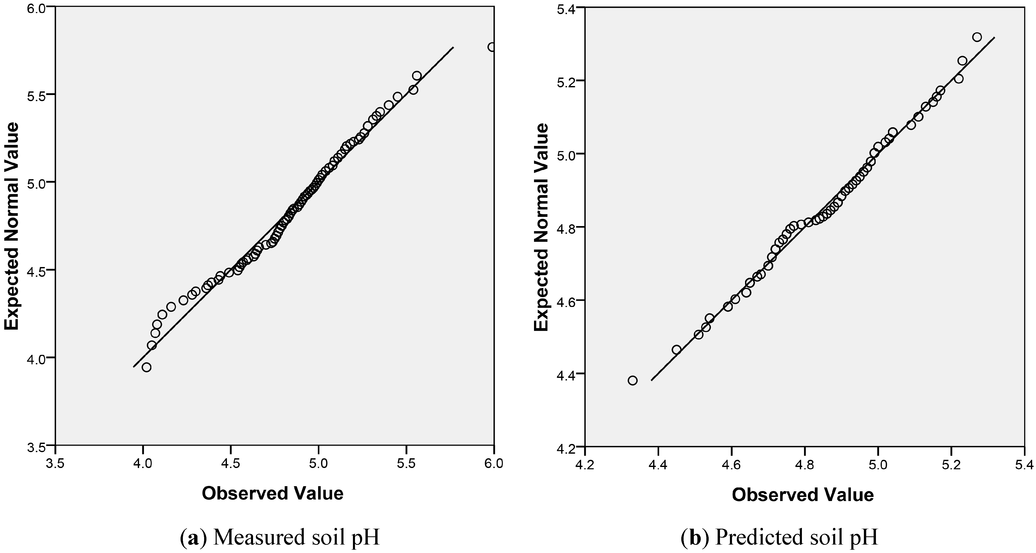
2.1. Summary Statistics

Table 1 shows the soil pH summary statistics for both the measured values at sampled locations and on the predicted surface. The mean measured value at sampled locations was 4.86 with a standard deviation of 0.34, indicating a tight cluster of values around the mean. The minimum soil pH was 4.02 while the maximum pH value was 5.56. The actual measured soil pH values were normally distributed as was shown by the mean and median which were approximately equal to each other and a coefficient of kurtosis of almost 3.00. The soil pH exhibited a crowding of lower values (4.0–4.5) in the central part of the study area with a south-west direction when mapped with an appropriate color scheme. The distribution of the measured soil pH and predicted soil pH is illustrated in the Q-Q plots shown in Figure 1a,b.

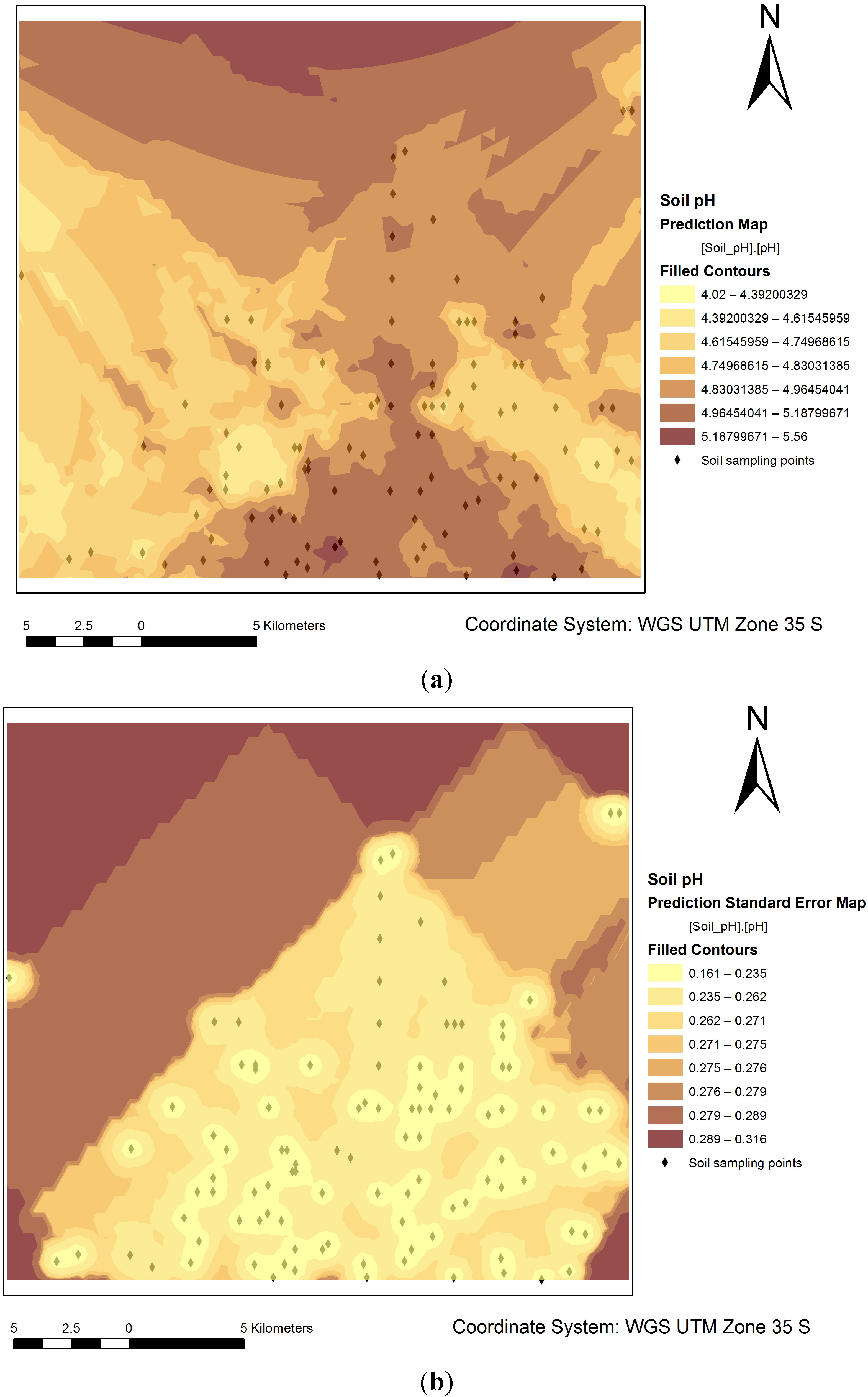
2.2. Kriging Interpolated Surface for Soil pH

The soil pH distribution map that was generated based on the measured data and fitted variograms is shown in Figure 2a while the prediction standard error map is shown in Figure 2b. It was clearly observed that the prediction variance was linked to the density of soil sampling data points. The highest prediction errors were observed in the northern-western direction which had a low sampling density. The associated summary statistics for the model predicted soil pH map were included in Table 1. Summary statistics of the predicted soil property values are discussed here as a first quality measure of the goodness of the model [9]. The mean soil pH value for the predicted surface was 4.86 while the median was 4.88, which were equal to those reported in the measured soil pH values. In addition, the first and third quartiles for predicted soil pH correspond to those that were observed in the measured soil pH. Further, the predicted soil property values followed the same distribution pattern as was observed in the measured values of soil pH.

Table 1. Summary statistics for measured and predicted soil pH.

Statistic	Measured Soil pH	Predicted Soil pH
Mean	4.86	4.86
Minimum	4.02	4.33
Maximum	5.56	5.28
Median	4.88	4.88
Standard deviation	0.34	0.18
1st Quartile	4.66	4.72
3rd Quartile	5.08	4.98
Skewness	−0.36	0.25
Kurtosis	3.11	2.89

Table 1. Summary statistics for measured and predicted soil pH.

Statistic	Measured Soil pH	Predicted Soil pH
Mean	4.86	4.86
Minimum	4.02	4.33
Maximum	5.56	5.28
Median	4.88	4.88
Standard deviation	0.34	0.18
1st Quartile	4.66	4.72
3rd Quartile	5.08	4.98
Skewness	−0.36	0.25
Kurtosis	3.11	2.89

Figure 1. Q–Q plot of measured and predicted soil pH

Figure 1. Q–Q plot of measured and predicted soil pH

The standard deviation in the predicted soil pH was 0.18 compared to 0.34 in the measured value indicating a tighter cluster of values around the mean in the predicted values. Generally, the soil pH did not have a definite pattern of distribution across the study area although it was noted that lower values (4.02–4.91) were predominant in the southern part of the study area. This might be attributed to continuous cultivation which was prevalent in this area compared to the northern part of the study area.

Figure 2. (a) Predicted soil pH map (b) Prediction standard error (soil pH).

Figure 2. (a) Predicted soil pH map (b) Prediction standard error (soil pH).

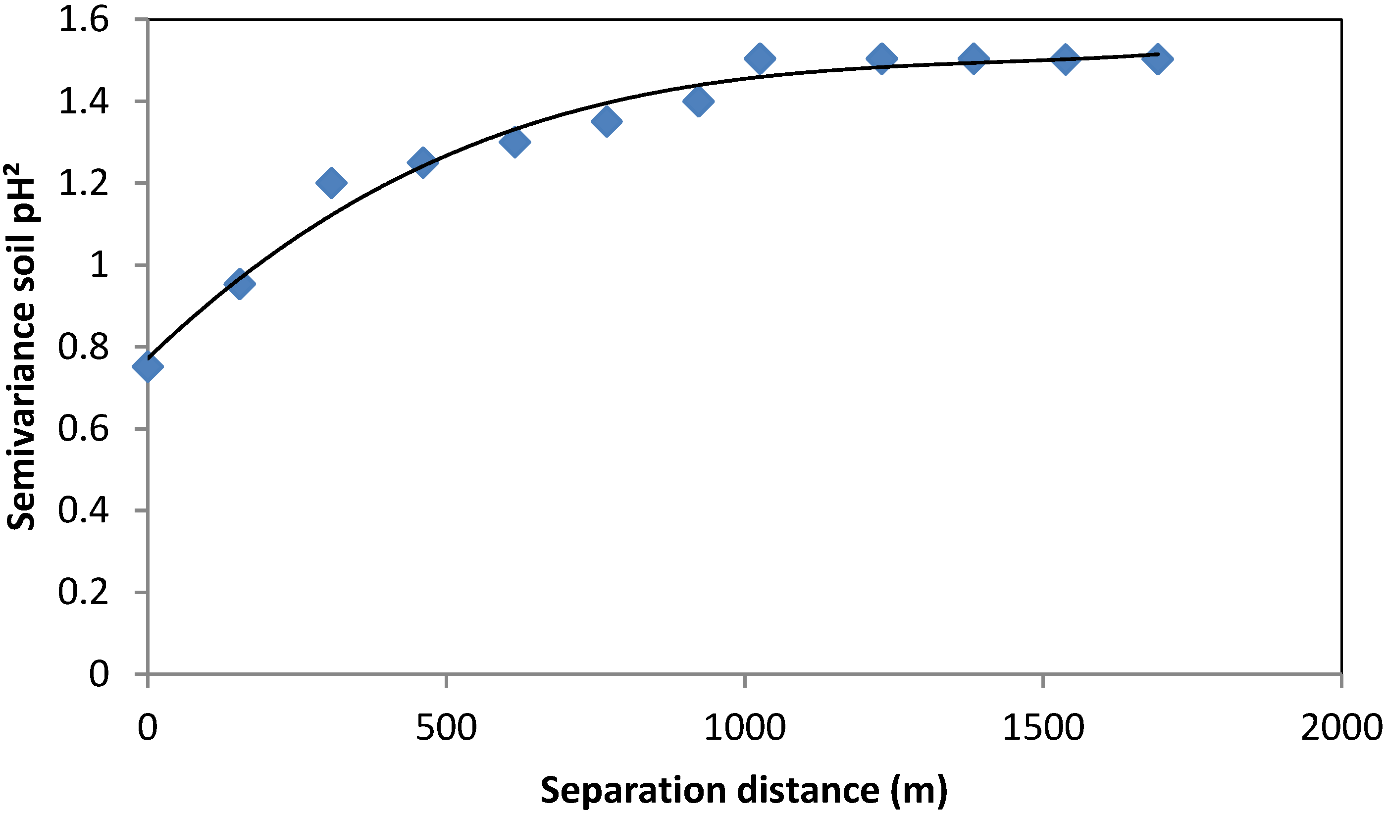
2.3. Spatial Autocorrelation for pH and Model Validation

The fitted experimental variogram is shown in Figure 3 and the associated variograhpic parameters are shown in Table 2. It was observed that the general spatial structure of soil pH along with the fitted spherical variogram was medium-as indicated by the nugget to sill ratio of 0.57 with a spatial dependence of up to 1379 m. The spherical nature of the fitted variogram suggests a constant pattern of variation of soil pH at the study site. It was further shown that soil pH varied more continuously across the study area as illustrated by the smaller nugget effect and larger range of its semivariogram. The spherical nature of the fitted variogram suggests a constant pattern of variation for soil pH at the study site.

Table 2. Fitted variogram parameters and prediction errors for OK model for prediction of soil pH.

Fitted Variogram Parameters
Nugget		Sill		Range (m)		Nugget/Sill Ratio
0.08		0.14		1379		0.57
Prediction Errors for OK Model Implemented to Predict Soil pH
Mean	Mean Standardized		RMSE		Average Standard Error		RMSE Standardized
−0.004	−0.008		0.36		0.39		0.93

Table 2. Fitted variogram parameters and prediction errors for OK model for prediction of soil pH.

Fitted Variogram Parameters
Nugget		Sill		Range (m)		Nugget/Sill Ratio
0.08		0.14		1379		0.57
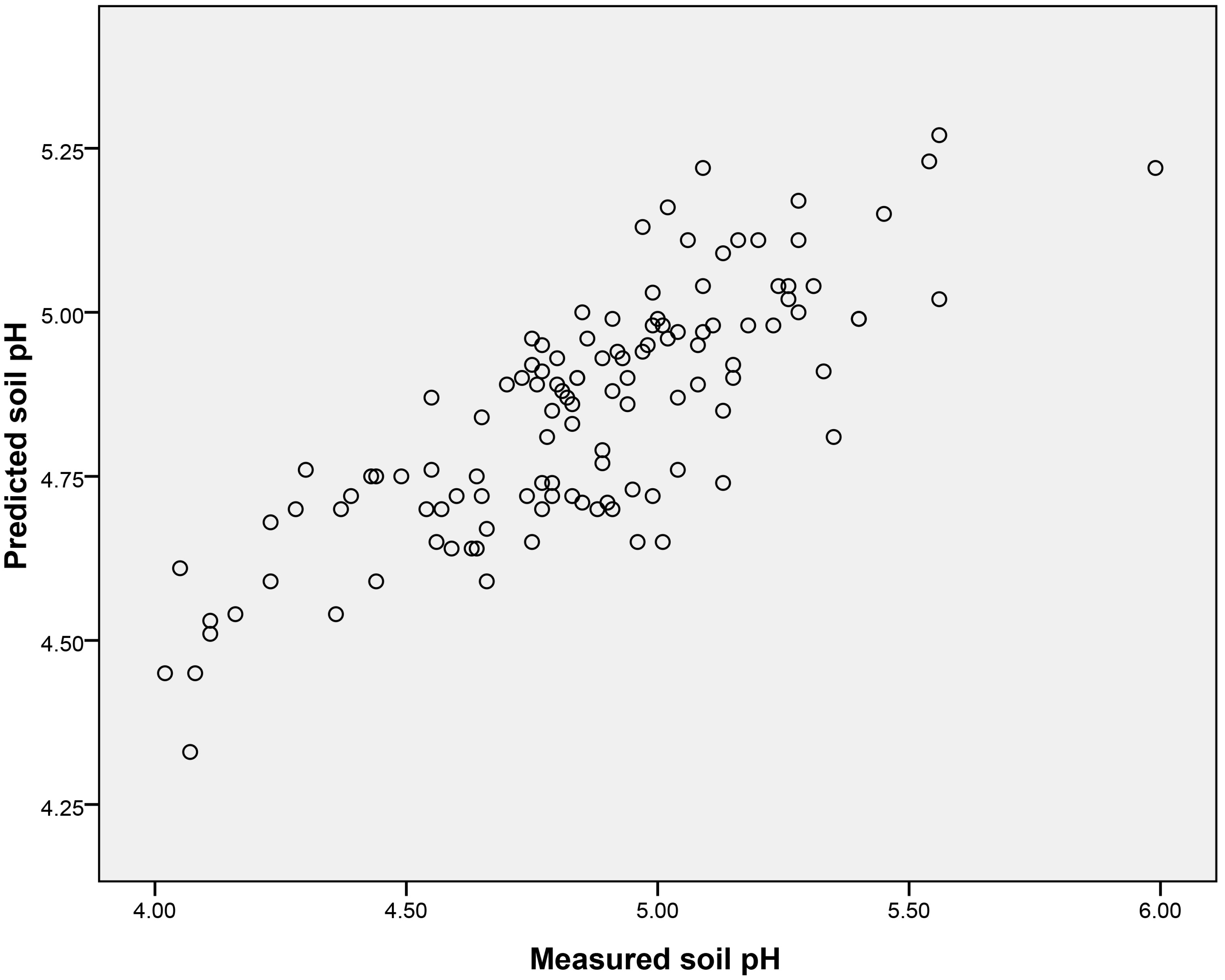
Prediction Errors for OK Model Implemented to Predict Soil pH
Mean	Mean Standardized		RMSE		Average Standard Error		RMSE Standardized
−0.004	−0.008		0.36		0.39		0.93

Figure 3. Fitted Variogram model for soil pH.

Figure 3. Fitted Variogram model for soil pH.

2.4. Model Validation

Based on the prediction errors (Table 2), the kriging model was judged as fair with a mean error of −0.004 and a standardized RMSE of 0.93. In addition, the average standard error (0.42) was close to the RMSE (0.38). These results show that the model was assessing the variability of predictions for soil pH from the true values fairly well. The map can thus be used as a guide for planning decisions regarding management of soil pH. This is because the model generated fairly well predicted and yet unbiased estimates of soil pH at locations that were not sampled. This is attested to by the cross plots of predicted pH values against measured values, which clustered around each other, indicating a significant positive relationship (Figure 4) with a correlation coefficient of 0.8. The study was compared with related work reported in literature. It is worth noting that literature close to the study area was very thin. One study at continental scale used regression kriging to create a digital soil map of pH for Europe, which revealed that there was a significant correlation between the estimated and the measured values with no significant difference (p = 0.05) between the measured and estimated values [4].

Figure 4. Cross plot of measured and predicted soil pH values.

Figure 4. Cross plot of measured and predicted soil pH values.

3. Experimental Section

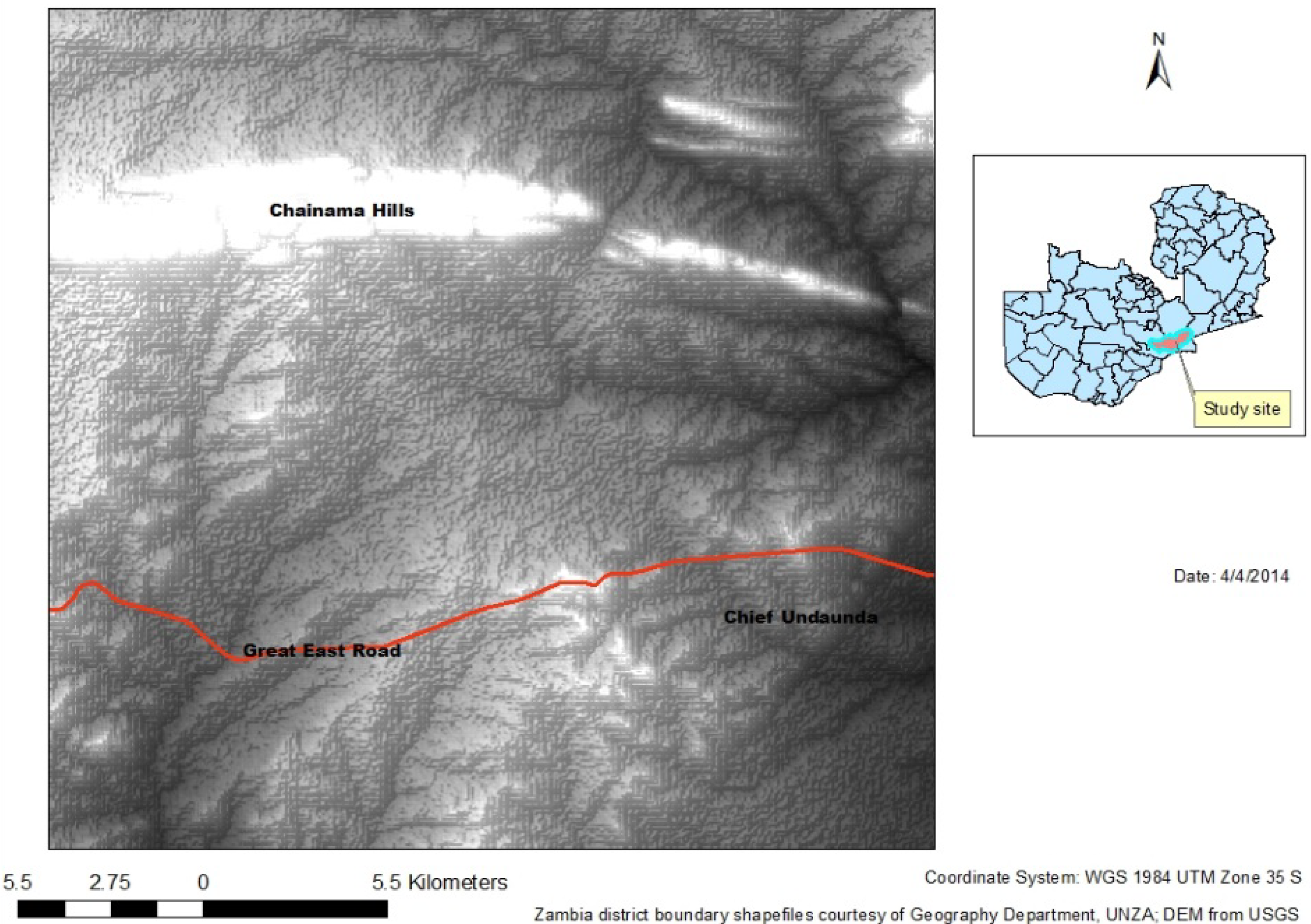
3.1. Study Area

The study site was located in the Chongwe-Rufunsa area in Lusaka Province of Zambia. It was located at longitudes 28°45′ E and 29°00′ E and latitudes 15°07′ S and 15°20′ S and covered parts of Munyeta and Mwapula local forest (Figure 5). It had an estimated area of 634 km². The geographic relief of the area is characterized by dambos, rivers and a plane plateau. The area has a distinct range of prominent hills known as the Chainama Hills transcending through the study site [10]. The elevations range from 970 to 1420 meters above sea level.

Figure 5. Location of study area.

Figure 5. Location of study area.

3.2. Soil Sampling and Laboratory Analysis

A total of 120 soil samples were collected from the 0–20 cm soil layer. The major limitation to soil sampling was accessibility. Therefore, to optimize the sampling strategy, the land form map was used to stratify clustered random sampling locations. The distance between soil sampling locations ranged from around 150 m up to 9500 m, although most of the sampling locations were separated by a distance of between 800 m and 1200 m. The location of soil sampling points are shown in Figure 2a. Five sub samples were taken at each location within a radius of 20 m and homogenized, after which a composite soil sample was taken and coded for laboratory analysis at the University of Zambia Soil Science Laboratory. The collected soil samples were first air-dried, ground where necessary and then passed through a 2 mm sieve to obtain the fine earth. The soil reaction represented by pH was determined in a 1:2.5 soil to solution ratio of 0.01 M CaCl₂ with a standard pH meter using the electrometric method as described by [11].

3.3. Data Pre-Processing and Analysis

The coordinates of the soil sampling points and the associated measured soil pH data were converted to shape files with coordinates in World Geodetic System 1984 (WGS 1984) zone 35 south. Preliminary screening of the measured soil pH data was done by drawing box plots of data sorted in three groups namely extremely acidic (4.0–4.5), strongly acid (4.5–5.0) and medium acidic (5.1–6.0). Outliers were identified visually as individually plotted rather than part of the whiskers in the box plots. The histogram tool in ArcGIS was also used. Where a more isolated bar from the main group of bars in the histogram was noted, the value was taken to represent a possible outlier. Where outliers were identified, the laboratory analyses were repeated after which box plots were redrawn. Where outliers were found, the soil pH measurement was repeated and in some cases the suspect values were removed. Thus, after this preliminary data screening, data for soil pH was represented by 119 soil samples. Summary statistics were then generated to provide a basic understanding of the characteristics of soil pH at the study site.

3.4. Geostatistical Analysis

Ordinary kriging (OK) was used to evaluate the spatial distribution of soil pH whose variogram was fitted globally. OK is one of the geostatistical models that use a set of statistical tools to predict the value of a given soil property at a location that was not sampled. Since OK relies on the assumption of stationarity, which requires in part that all data values come from distributions that have the same variability, the data was examined further to ascertain the kind of data preprocessing that was necessary for efficient model implementation. The soil pH data set was first mapped using an appropriate color and classification scheme to check if there was any pattern associated with the soil pH. The classification scheme comprised three classes, namely extremely acidic (4.0–4.5), strongly acid (4.5–5.0) and medium acidic (5.1–6.0).

Additional data evaluation was done using the histogram, the normal QQ plot and the trend analysis tools. The histogram and normal QQ plot tools were used to analyze the distribution of the measured soil pH data. This exploration showed that the soil pH data was normally distributed and thus no transformation was performed on it.

The trend analysis tool was used to check if a non-random trend was present in the soil pH data. Since a spatial trend was found, a second order polynomial was fitted to the data so as to remove the trend. Removing the trend in this way allowed for it to be modeled separately; and added back in the final output, it enabled optimization of model performance in the prediction of soil pH.

The theory and principles applicable to OK kriging have been described in detail by various authors [12,13,14]. In summary, OK is said to be an exact interpolator in the sense that interpolated values or their local average coincide with values at the sampled locations. The predicted soil pH Ẑ(x₀), at an unsampled location s₀ using observations Z(x_i), i = 1,..., n was given by:

$$\text{Ẑ}\left(x_0\right)={\displaystyle \sum }_{i=1}^n{\lambda }_i.Z\left(x_i\right)$$

where λ_i is the kriging weight.

This model incorporated the spatial coordinates of soil sampling points in the data processing, thus allowing description and modeling of spatial patterns and evaluation of uncertainty or error attached to the predictions [12]. The spatial variation was quantified by the semivariance, which is half the expected squared difference between the soil property values at two locations [12]. A spherical semivariogram model was automatically fitted using the weighted least square procedure. The variograms parameters of nugget, sill and range were used to indicate the spatial nature [15] of soil pH at the study site. In addition, the nugget to sill ratio was reported to indicate the ratio of random (unexplained) variation to total variation.

All data processing and analysis was done in ArcGIS 10.1 [16].

3.5. Validation of Spatial Prediction of Soil pH

Cross validation and true validation were used to evaluate the accuracy of the predicted soil pH. Further checking was done by evaluating soil pH values at the sampled locations in a cross plot of predicted and measured values and assessing the distribution of predicted values and the associated summary statistics [10]. During cross validation, each of the sampled locations was removed one at a time and the associated soil pH value at that location predicted using the five surrounding values. The predicted and actual values were then compared. The quantitative model assessment measures were prediction errors, namely, the mean error, root mean square error, average standard error and mean standardized error. The goal was to have a model with an average error and standardized mean prediction error close to zero. Further, if the average standard errors were close to the root mean squared prediction errors, then the model was said to have correctly assessed the variability in the predictions. In addition, the root mean squared standardized error had to be close to one (1) if the model was correctly estimating the variability.

4. Conclusions

This study has demonstrated the application of geo-statistical procedures to the mapping of soil pH in Zambia. The kriging model-that was developed was found to be satisfactory with a low spatial autocorrelation and a nugget to sill ratio of 0.85. Model validation and assessment revealed fair performance in the generation of predicted values with acceptable prediction errors and overall map accuracy of 56.00%. Therefore, the generated soil map can serve as a proxy for soil pH in Zambia, where evidence of spatial structure and quantitative estimates of uncertainty are reported. Thus, the map produced can be used as guide for various uses, including identifying lime application rates according to spatial variability of soil pH. However, to more precisely understand what is driving soil pH variability in this system, further research should be done to include data sets representing factors of soil formation.

References

1. Caritat, P.; Cooper, M.; Wilford, J. The pH of Australian Soils; Field Results from a National Survey. Soil Res. 2011, 49, 173–182. [Google Scholar] [CrossRef]
2. Bickelhaupt, D. What is Soil pH: What It Means. Available online: http://www.esf.edu/pubprog/brochure/soilpH (accessed on 13 January 2014).
3. Schirrmann, M.; Gebbers, R.; Seidel, E.K.E. Soil pH Mapping with an On-the-go Sensor. Sensors 2011, 11, 573–598. [Google Scholar] [CrossRef]
4. Reuter, H.I.; Lado, L.R.; Hengl, T.; Montanarella, L. Continental—Scale Digital Soil Mapping Using European Soil Profile Data: Soil pH. Hamburger Beitrage zur Physischen Geographie und Landschaftokologie-Heft19. 2008. Available online: http://www.academia.edu/587354/continetal_scale_digital (accessed on 20 January 2014).
5. Sheng, J.; Ma, L.; Jiang, P.; Li, B.; Huang, F.; Wu, H. Digital Soil Mapping to Enable Classification of the Salt Affected Soils in Desert Agro-ecological Zones. Agric. Water Manag. 2010, 97, 1944–1951. [Google Scholar] [CrossRef]
6. Connolly, J.; Holden, N.M.; Ward, S.M. Mapping Peatlands in Ireland Using a Rule-based Methodology and Digital Data. SSSAJ 2007, 71, 492–499. [Google Scholar] [CrossRef]
7. Robinson, T.P.; Metternicht, G. Testing the Performance of Spatial Interpolation Techniques for Mapping Soil Properties. Comput. Electron. Agric. 2006, 50, 97–108. [Google Scholar] [CrossRef]
8. Mambo, A.; Phiri, L.K. Soil Acidity Map of Zambia; Zambia Agriculture Research Institute: Lusaka, Zambia, 2004. [Google Scholar]
9. Leungthong, O.; McLennan, J.A.; Deutsch, C.V. Minimum Acceptance Criteria for Geostatistical Realizations. Nat. Resourc. Res. 2004, 13, 131–141. [Google Scholar] [CrossRef]
10. Chabala, L.M.; Mulolwa, A.; Lungu, O. Landform Classification for Digital Soil Mapping in the Chongwe-Rufunsa Area, Zambia. Agric. For. Fish. 2013, 2, 156–160. [Google Scholar]
11. McNeal, E.O. Soil pH measurements. In Methods of Soil Analysis Part 2; Page, A.L, Keeney, D.R., Miller, R.H., Eds.; Soil Science Society of America, Inc.: Madison, WI, USA, 1982. [Google Scholar]
12. Burrough, P.A.; McDonnell, R.A. Principles of Geographical Information Systems; Oxford University Press: New York, NY, USA, 2004; p. 190. [Google Scholar]
13. Chahouki, M.A.A.; Chahouki, A.Z.; Ahvasi, L.K. Comparing Geostatistical Approaches for Mapping Soil Properties in Poshtkouh Rangelands of Yazd Province, Iran. Vegetos 2011, 24, 77–88. [Google Scholar]
14. Johnston, K.; ver Hoef, J.M.; Krivoruchko, K.; Lucas, N. Using ArcGIS Geostatistical Analyst; ESRI Press: Redlands, CA, USA, 2001. [Google Scholar]
15. Cambardella, C.A.; Moorma, T.B.; Novak, J.M.; Parkin, T.B.; Karlen, D.L.; Turco, R.F.; Konopka, A.E. Field Scale Variability of Soil Properties in Central Iowa soils. Soil Sci. Soc. Am. J. 1994, 58, 1501–1511. [Google Scholar] [CrossRef]
16. Environmental Systems Research Institute (ESRI). ArcGIS Desktop; Environmental Systems Research Institute: Redlands, CA, USA, 2011. [Google Scholar]