Article

Early Identification of Corn and Soybean Using Crop Growth Curve Matching Method

1
State Key Laboratory of Efficient Utilization of Arid and Semi-Arid Arable Land in Northern China, The Institute of Agricultural Resources and Regional Planning, Chinese Academy of Agricultural Sciences, Beijing 100081, China
2
Digitization and Informatics Division, Food and Agriculture Organization of the United Nations, 00153 Rome, Italy
*
Author to whom correspondence should be addressed.
Agronomy 2024, 14(1), 146; https://doi.org/10.3390/agronomy14010146
Submission received: 14 December 2023 / Revised: 1 January 2024 / Accepted: 7 January 2024 / Published: 8 January 2024

Abstract

:
The prompt and precise identification of corn and soybeans are essential for making informed decisions in agricultural production and ensuring food security. Nonetheless, conventional crop identification practices often occur after the completion of crop growth, lacking the timeliness required for effective agricultural management. To achieve in-season crop identification, a case study focused on corn and soybeans in the U.S. Corn Belt was conducted using a crop growth curve matching methodology. Initially, six vegetation indices datasets were derived from the publicly available HLS product, and then these datasets were integrated with known crop-type maps to extract the growth curves for both crops. Furthermore, crop-type information was acquired by assessing the similarity between time-series data and the respective growth curves. A total of 18 scenarios with varying input image numbers were arranged at approximately 10-day intervals to perform identical similarity recognition. The objective was to identify the scene that achieves an 80% recognition accuracy earliest, thereby establishing the optimal time for early crop identification. The results indicated the following: (1) The six vegetation index datasets demonstrate varying capabilities in identifying corn and soybean. Among those, the EVI index and two red-edge indices exhibit the best performance, all surpassing 90% accuracy when the entire time-series data are used as input. (2) EVI, NDPI, and REVI2 indices can achieve early identification, with an accuracy exceeding 80% around July 20, more than two months prior to the end of the crops’ growth periods. (3) Utilizing the same limited sample size, the early crop identification method based on crop growth curve matching outperforms the method based on random forest by approximately 20 days. These findings highlight the considerable potential and value of the crop growth curve matching method for early identification of corn and soybeans, especially when working with limited samples.

1. Introduction

Precise and timely mapping of crop distribution is indispensable for agricultural monitoring and decision-support applications, encompassing crucial tasks, such as crop yield estimation, optimization of crop planting structures, early detection of crop disasters, agricultural insurance, and land leasing [1,2,3,4]. This mapping is pivotal not only for the efficiency of agricultural management but also for guaranteeing food security [5,6,7]. Remote sensing-based methods for crop identification have become essential tools for crop-type recognition, playing a crucial role in various early detection systems in agriculture [7,8].
At present, scholars have extensively investigated crop-type identification using a variety of remote sensing data sources [9,10]. The integration of multi-temporal remote sensing data, coupled with spectral and temporal information, enhances the monitoring of crop growth variations throughout the growing season and improves crop-type recognition [11,12]. Despite these advancements, many studies necessitate complete time-series data for an entire growing season, resulting in a delay of several months or even a year in obtaining crop-type information and distribution mapping after the conclusion of the growing season. This delay hinders the timely and practical significance of crop monitoring for scientific agricultural management, including irrigation scheduling and yield estimation [13,14,15]. Current methods for identifying crop types often require extensive ground samples for training and validation, leading to inefficiencies, especially in large-scale crop remote sensing monitoring, where sample scarcity is a common challenge [16]. Therefore, early crop identification research has gained increasing attention [17,18,19,20,21,22]. This involves obtaining information on crop-type distribution several months before the end of the growing season to meet the actual needs of agricultural management. Simultaneously, early identification of crop types implies the absence of complete remote sensing data for the entire growing season. Moreover, the limited number of input images and the necessity to reduce reliance on ground survey samples impose higher requirements on the selection of data sources and identification methods for early crop identification [23].
In early crop identification research, it is customary to leverage the characteristic differences in the time-series data of different crops. These distinctions become evident early in the time series, emphasizing the need for time-series data sufficient temporal density. Moderate-Resolution Imaging Spectroradiometer (MODIS) data, re-known for their daily observation capabilities, have been widely employed in early crop identification [24,25,26,27]. Skakun utilized historical MODIS-derived Normalized Difference Vegetation Index (NDVI) data and a Gaussian mixture model (GMM) to distinguish winter crops from spring and summer crops in the state of Kansas in the US and Ukraine [26]. The results revealed accuracy exceeding 90%, achievable almost two months before the winter crop harvest, presenting an opportune timeframe for crop distribution mapping. Nevertheless, the utilization of low spatial resolution imagery like MODIS may inevitably result in misclassification and omission errors owing to mixed pixels. Therefore, data with higher spatiotemporal resolution would be more applicable in early crop identification [28,29]. In a study by You and Dong, the Google Earth Engine (GEE) platform, in conjunction with Sentinel-1/2 imagery, was employed for the early identification of crops, such as rice, maize, and soybean. This investigation generated crop distribution maps for the current year with an overall accuracy of 0.91 by combining historical images and ground survey samples using a random forest classifier [17]. In a related study, Wei conducted research to identify rice, maize, and soybean early using Sentinel-2A/B data on the GEE platform, achieving an accuracy exceeding 90% [30]. The study compared the effectiveness of different vegetation indices combined with various deep learning algorithms for early identification. Utilizing high-spatial-resolution data, these studies have the potential to enhance the accuracy of crop-type identification. However, they often require sufficient samples for model training, limiting their applicability in research areas with a scarcity of samples. Certain studies have used data with higher spatiotemporal resolution for crop identification. For example, Gao utilized VENμS satellite imagery to identify maize and soybean at the sub-field scale. However, the prohibitive cost of acquiring data from commercial satellites renders them unsuitable for large-scale crop distribution mapping studies [31].
Currently, widely used data sources with higher spatial resolution include Landsat and Sentinel-2 data [32,33,34,35]. Both datasets are publicly accessible and share comparable spatial resolutions. The National Aeronautics and Space Administration (NASA) initiated the Harmonized Landsat and Sentinel-2 (HLS) dataset, which combines Landsat 8 and Sentinel-2 data to generate surface reflectance data with high spatial and temporal resolutions [36]. Many scholars have leveraged HLS products for remote sensing studies, such as monitoring dynamic changes in grassland landscapes and mapping crop planting frequencies [37,38]. Due to its optimal temporal density and spatial resolution, the HLS dataset holds significant potential for further applications in early crop identification research.
Numerous previous classification studies have progressively embraced machine learning algorithms, such as random forest (RF), support vector machine (SVM), and convolutional neural networks (CNNs), known for their efficacy in various classification tasks [39,40,41,42]. In contrast, this study adopts a novel approach to crop identification based on evaluating the similarity between time-series data and crop growth curves. This method aims to reduce dependence on ground samples and eliminate the need for intricate algorithm parameter configurations. The objectives of this study are as follows: (1) utilize the high spatiotemporal resolution and multi-band advantages of the HLS dataset for research on the identification of corn and soybean types; (2) generate various vegetation index datasets to ascertain the optimal vegetation index type for enhancing crop identification accuracy; (3) pinpoint the earliest time range for both crops with high classification accuracy by configuring various scenarios with distinct input image data.

2. Materials and Methods

2.1. Study Area

The study area is situated in DeKalb County, northern Illinois, USA, covering an area of approximately 1645 square kilometers (Figure 1). Illinois stands as a leading agricultural state in the United States, with 80% of its land dedicated to agricultural purposes. The average cultivated land per household is 140 hectares (around 2100 acres), predominately featuring major crops such as corn and soybeans.
Illinois exhibits a flat topography with an average elevation of 182 m, sloping gradually from north to south. The northwestern region showcases slightly elevated terrain characterized by gently rolling hills, reaching the state’s highest point at an elevation of 378 m. The climate in Illinois is classified as temperate, marked by cold and snowy winters and hot summers. The average winter temperatures in the northern part hover around −6 °C, while in the southern part, they reach approximately 3 °C. The summer temperatures average at 21 °C in the north and 25 °C in the south. Annual precipitation averages between 800–1200 mm in the north and 1200–1600 mm in the south. The growing season for crops in the south spans 210 days, while in the north it is limited to 160 days.

2.2. Data and Processing

2.2.1. HLS Data Collection

The Harmonized Landsat and Sentinel-2 (HLS) project, initiated by the National Aeronautics and Space Administration (NASA), aims to leverage data from the Operational Land Imager (OLI) and Multispectral Instrument (MSI) aboard Landsat 8 and Sentinel-2 satellites. The goal of this project is to generate consistent and unified surface reflectance products. The integration of these two sensors enables global observations of the Earth’s surface at a spatial resolution of 30 m every 2–3 days. The resultant data products undergo a standardized preprocessing pipeline, encompassing atmospheric correction, cloud and cloud shadow masking, spatial co-registration, normalization of illumination and viewing angles, and spectral bandpass adjustment. This meticulous process ensures that HLS becomes a stackable and comparable seamless time-series product. The dense time series afforded by HLS facilitates unprecedented monitoring of dynamic surface properties with exceptional spatial detail [36]. The heightened temporal resolution of this dataset holds substantial potential to significantly benefit studies on land cover change, agricultural management, disaster response, water resources, and vegetation phenology.
To assess and analyze the identification performance of various vegetation index data, such as the red edge vegetation index, this study exclusively utilizes the S30 product from the HLS dataset. This product is derived from Sentinel-2A and Sentinel-2B MSI data. The data acquisition period for this study spans from 4 April to 7 November 2021, corresponding to the 94th to 311th day of the year (DOY), covering a duration of 218 days. Throughout this timeframe, more than 100 HLS-S30 data acquisitions were conducted. Following the consideration of data processing (see details in Section 2.2.3), a total of 40 images were ultimately deemed usable (Table 1).

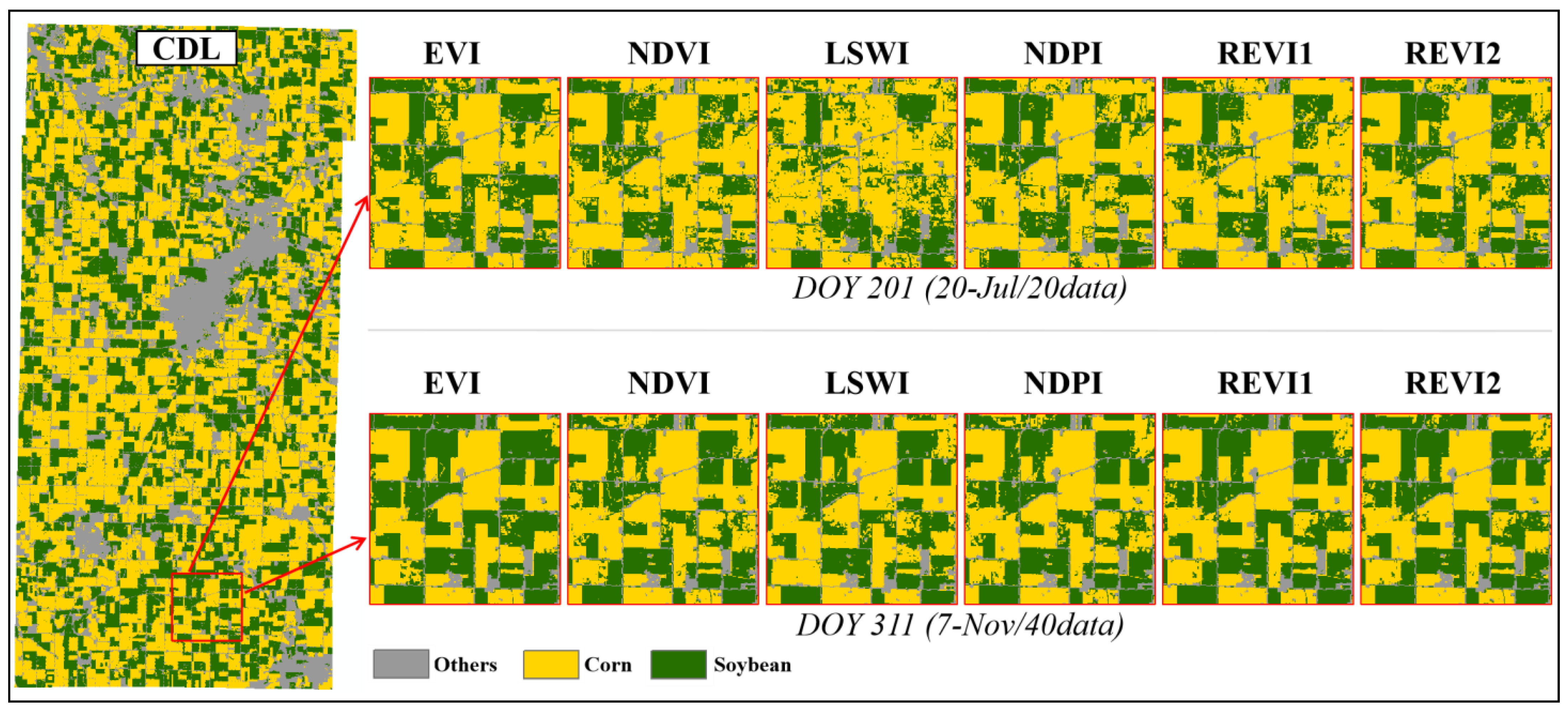
2.2.2. CDL Data Collection

The Cropland Data Layer (CDL) dataset is an annual land cover remote sensing product publicly released by the United States Department of Agriculture (USDA). This product has a 30 m spatial resolution and utilizes data from various satellites, including the Advanced Wide-Field Sensor (AWiFS), Landsat Thematic Mapper/Enhanced Thematic Mapper Plus (TM/ETM+), Deimos-1, UK-DMC-2, and Moderate-Resolution Imaging Spectroradiometer (MODIS). The ground reference data used to categorize agricultural and non-agricultural land in the CDL product are derived from the Common Land Unit (CLU) data, as disseminated by the USDA’s Farm Service Agency (FSA), and the 2001 National Land Cover Database (NLCD2001) data. The CLU-based data are collected during each growing season, when producers furnish details on crop types and corresponding areas within their farmland to the FSA county offices. In an overarching assessment, the CDL product exudes a robust level of confidence in its classification accuracy. Covering a range of more than 100 crop types, the CDL dataset attains a classification accuracy surpassing 90% for major crops, like corn, soybeans, and winter wheat [43]. Its widespread application extends to domains such as land use and land cover change as well as agricultural monitoring [44,45].

2.2.3. Data Processing

This study employed a process to obtain HLS data in R, following the workflow outlined by the E-Learning platform (https://lpdaac.usgs.gov/resources/e-learning/ (accessed on 7 January 2024)). This platform is collaboratively managed by the US Geological Survey (USGS) and NASA as part of the joint project known as Land Processes Distributed Active Archive Center (LP DAAC). The HLS products, stored as GeoTIFF files optimized for cloud storage and distribution, are archived and disseminated by LP DAAC. To facilitate the retrieval of HLS data without downloading the source data, this study utilized the NASA CMR-STAC (Collection for STAC) Application Programming Interface (API). In the initial step, administrative vector data for the state and county levels of Illinois in the United States (Figure 1) were acquired from a public database, GDAM (https://gadm.org/ (accessed on 7 January 2024)). Subsequently, the vector file of DeKalb county was converted into a geojson format file within RStudio, defining the study area’s scope. After setting the time range for image acquisition, this study omitted the imposition of a cloud coverage filter but instead employed HLS’s Quality Assessment (QA) layer generated from the Fmask algorithm [46] to conduct cloud processing on all queried data. Within the HLS framework, both values of 0 and 64 in the QA layer denote pixels devoid of cloud, cloud shadow, water, or snow/ice. To enhance the retention of usable pixels, this study conducted a comparative analysis of masked images generated using different quality control schemes against the original images captured on the respective day. The final recommendation in this study involved preserving specific QA layer values, such as 0, 4, 64, 68, 100, 128, 132, and 192, as benchmarks for masking. Subsequently, the mask function is applied in the calculation project to compute six vegetation index data through the formulas presented in Section 2.3.1. The final results are then saved locally for further analysis. Throughout the growing season, approximately 100 sets of masked images were computed for each vegetation index dataset. Subsequently, through visual assessment, masking areas were determined to be less than approximately 50%. Considering factors such as time distribution and the spatial distribution of the masks, 40 images were ultimately chosen as the input data representing the entire growing season.
The CDL data utilized in this study were sourced from the USDA’s National Agricultural Statistics Service (https://nassgeodata.gmu.edu/CropScape/ (accessed on 7 January 2024)). This platform allows for the customization of the research area, year, crop type, projection coordinates, and other parameters for data retrieval. The CDL images selected cover the study area, as depicted in Figure 1, and maintain consistency in projection information and spatial resolution with HLS data, specifically WGS84-UTM 16N and 30 m, respectively. To ensure complete spatial registration with HLS data, the CDL image is then cropped to match the size of HLS data using the same vector file for DeKalb county. Simultaneously, given the study focused on corn and soybeans, all other land feature types were amalgamated into the ‘others’ category (Figure 1).

2.3. Methods

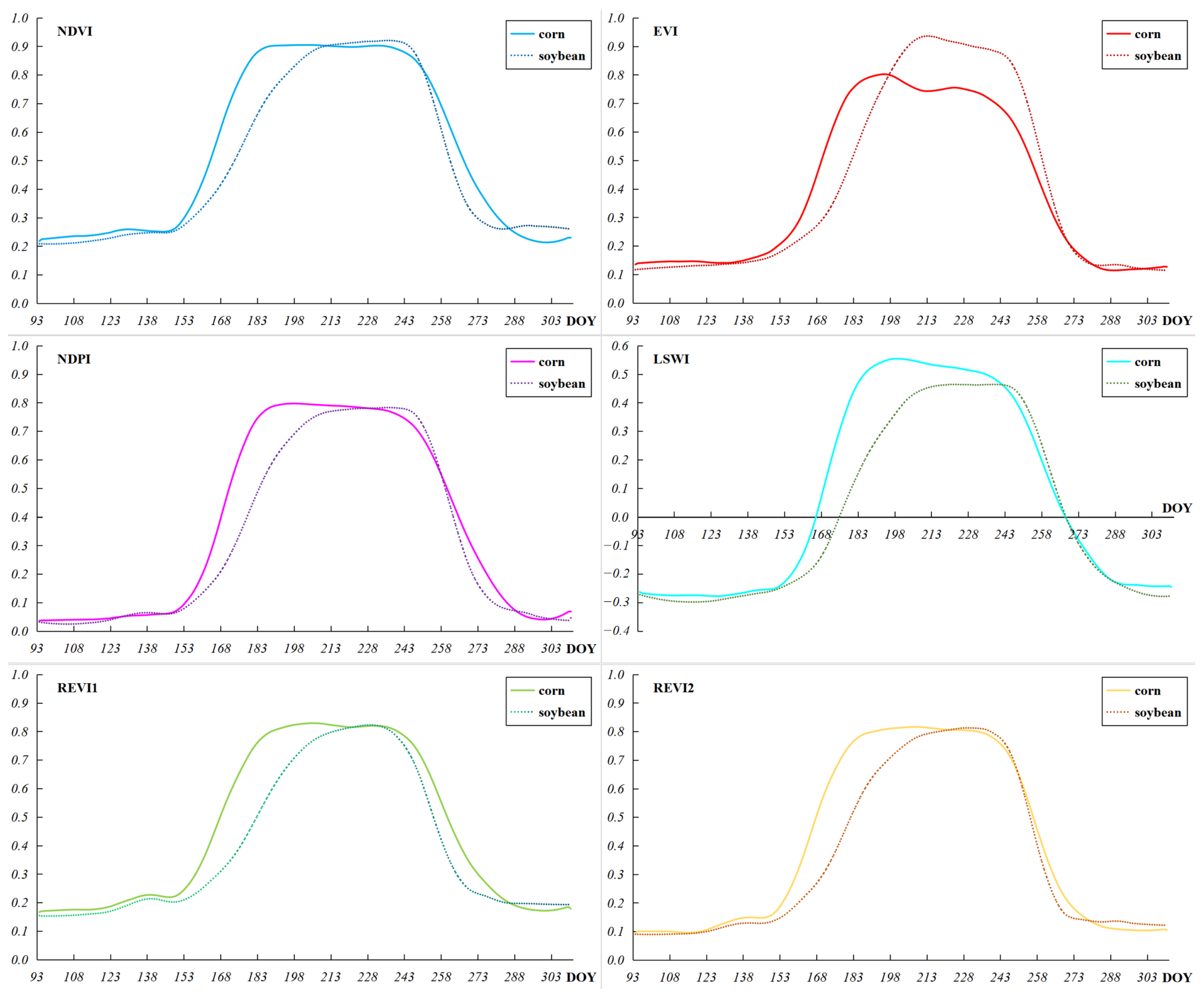
2.3.1. Construction of Vegetation Indices

This study developed six vegetation indices using various bands from the HLS-S30 product, categorized into three general categories. Firstly, common indices like NDVI and EVI (Enhanced Vegetation Index), which combine visible and near-infrared bands, were chosen due to their proven effectiveness in distinguishing crop types [47,48]. In comparison to NDVI, EVI exhibits superior discrimination effects when most crops have low to medium green biomass, such as during the greening stage and senescence stage, while NDVI’s classification sensitivity diminishes under high green biomass levels [49,50].
The second type employs LSWI (Land Surface Water Index) and NDPI (Normalized Difference Phenology Index) in the shortwave infrared band (SWIR). Previous studies have demonstrated that the SWIR band possesses a better ability to differentiate between corn and soybeans compared to the visible bands [17,32]. LSWI serves as a reliable indicator of vegetation moisture content and captures the unique spectral characteristics of soil, water, and open canopy during the early stages of crop growth [51]. NDPI exhibits higher sensitivity to vegetation growth, particularly when vegetation growth and snowmelt coincide, making NDPI more effective than NDVI in monitoring spring plant phenology [52].
The third category encompasses two widely used red-banded vegetation indices, named REVI1 (Red Edge Vegetation Index 1) and REVI2 (Red Edge Vegetation Index 2) in this study. Existing research indicates that red-edge bands and shortwave infrared bands are expected to provide crucial information about vegetation [53]. Among the three red-edge bands of Sentinel-2/MSI, the first red-edge band (re1) is most influenced by chlorophyll content, followed by the second red-edge band (re2), with the third red-edge band (re3) having minimal impact [54]. Consequently, to maximize differentiation, this study selected the re1 and re3 bands when constructing the red-edge index. The calculation formulas for the six vegetation indices are as follows.
N D V I = ρ n i r ρ r e d ρ n i r + ρ r e d
E V I = 2.5 × ρ n i r ρ r e d ρ n i r + 6 × ρ r e d 7.5 × ρ b l u e + 1
L S W I = ρ n i r ρ s w i r 1 ρ n i r + ρ s w i r 1
N D P I = ρ n i r ( 0.74 × ρ r e d + 0.26 × ρ s w i r 1 ) ρ n i r + ( 0.74 × ρ r e d + 0.26 × ρ s w i r 1 )
R E V I 1 = ρ n i r ρ r e 1 ρ n i r + ρ r e 1
R E V I 2 = ρ r e 3 ρ r e 1 ρ r e 3 + ρ r e 1
In the above formulas, ρ b l u e , ρ r e d , ρ r e 1 , ρ r e 3 , ρ n i r , ρ s w i r 1 , respectively, represent the reflectivity of the B02, B04, B05, B07, B8A, and B11 (Table 2). These six vegetation index data were calculated in R and have the same distribution range, resolution, and spatial reference, with the value ranging between [17,32].

2.3.2. Extraction of Crop Growth Curves

During the crop growth period, which spanned 218 days, we calculated 40 periods of data for each vegetation index. In order to obtain a time-continuous complete vegetation index curve and use it for subsequent crop growth curve extraction, this study uses a flexible fitting (Flexfit) algorithm to fill in the missing data between the 40 periods of data for each vegetation index to generate daily continuous vegetation index data [31]. The Flexfit method is capable of addressing significant temporal gaps within time-series data, facilitating both data noise elimination and data smoothing. Diverging from conventional Savitzky–Golay (SG) filtering methods reliant on fixed time windows, the Flexfit tool exhibits versatility by employing more extensive time windows. This flexibility proves particularly advantageous for accommodating the 40-day period under examination in this study, wherein period data are extrapolated to yield a complete daily dataset spanning 218 days. Following rigorous testing, the parameters for Flexfit fitting in this study were established as follows: the spike threshold, increase weight, and number of iterations for filling large gaps were set to 3, 2, and 3, respectively. Additionally, the minimum number of samples for smoothing was determined to be 5, while the maximum search window size was capped at 60. Subsequently, we randomly selected 20 sample points for corn and soybean utilizing the confidence layer of CDL data with confidence levels surpassing 0.95. These sample points were then overlaid onto the fitted time-series vegetation index data to extract 20 curves for each crop. Following a meticulous screening process, certain curves whose shapes deviated from the majority, owing to poor fitting results, were eliminated. Ultimately, only 10 curves were retained as crop growth curves for each crop. Figure 2 illustrates the average crop growth curve of the six vegetation indices for enhanced presentation.

2.3.3. Classifier and Accuracy Assessment

For each pixel, the 40 periods of vegetation index values are organized chronologically, and the shapes of these 40 values are compared against a total of 20 extracted crop growth curves for both crops. If the similarity between the pixel’s 40 data value and a particular curve is the highest, the crop-type information for that pixel is determined by assessing whether the curve corresponds to the corn or soybean growth curve. This pixel-wise evaluation results in obtaining crop-type information for all pixels within the entire study area. The process of similarity matching between pixel values and curves adheres to a logical sequence and can be represented by the following formula [30]. The process of crop classification involves comparing the data value of each pixel to all growth reference curves. Then, the curve with the smallest difference is considered a match, and the crop attributes of that growth curve are used to determine the type of crop planted at the pixel location. This process of similarity matching between pixel values and curves adheres to a logical sequence [55] and can be represented by the following formula.
L ( x ) = a     M ( x + x 0 ) + b
Here, L ( x ) denotes the HLS time-series vegetation index curve function, M ( x ) represents the optimal crop growth curve function, x signifies a specific day within the growing season, x 0 represents the time offset (within the range of ±10 days, as set in this study), and a and b are fitting parameters determined using the least square method. By systematically comparing the variation between the vegetation index data and the growth curves on a pixel-by-pixel basis, the curve exhibiting the highest R2 value is identified as the optimal growth curve, highlighting the best similarity.
In the assessment of crop classification performance, the overall accuracy serves as the criterion for evaluating the effectiveness of various vegetation indices in classification. In this study, corn and soybean distribution information from the CDL classification map with high confidence is utilized as verification data to compare spatial positions and pixel counts with the identification results obtained through the crop growth curve matching method. This accuracy assessment strategy, employing CDL data as verification data, is also extended to the evaluation process of random forest classification outcomes in Section 3.2.

3. Results

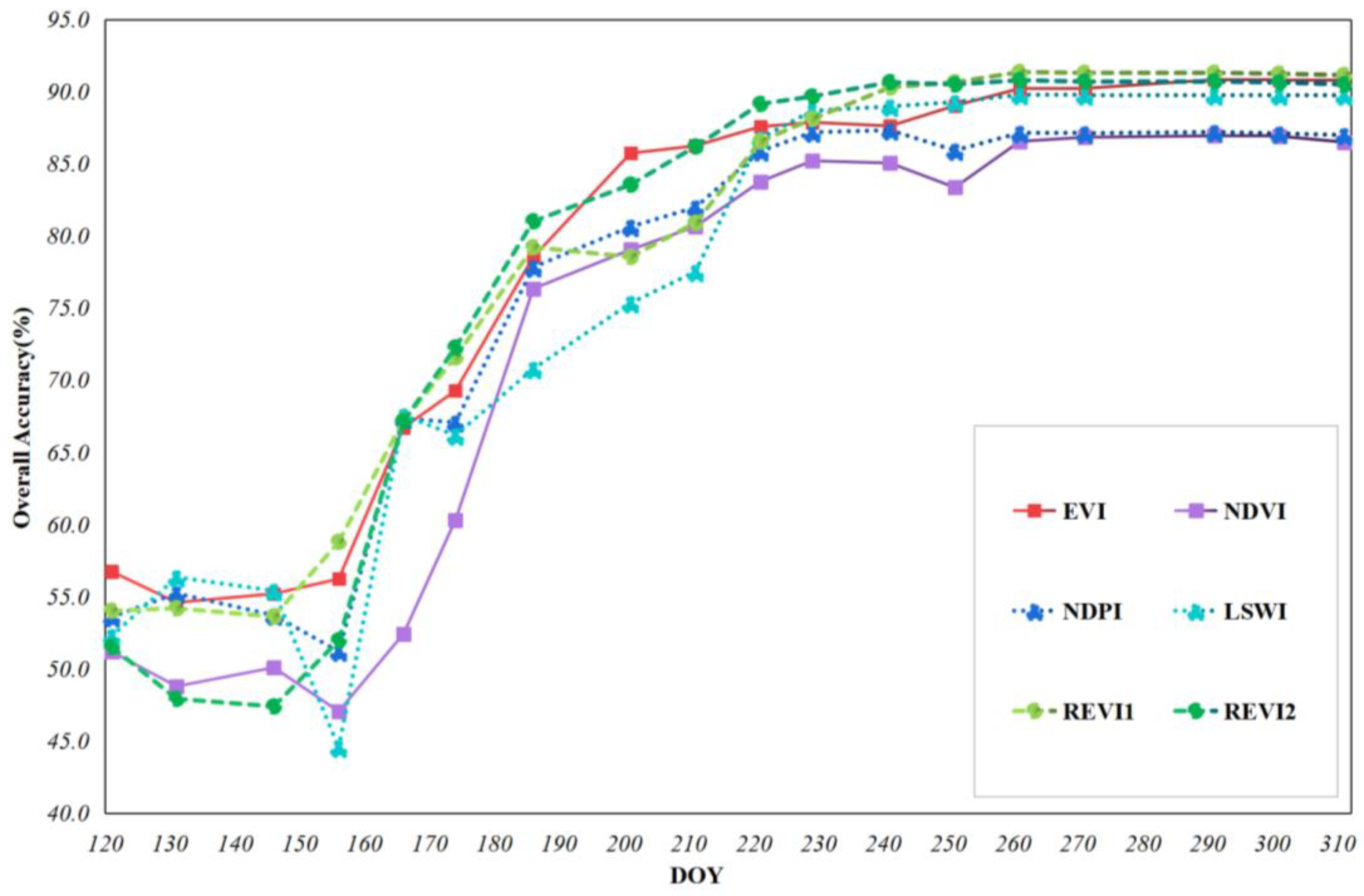
3.1. Identification Performance of the Six Indices

When utilizing a dataset comprising 40 periods of vegetation index data throughout the entire growing season for crop-type identification, all six vegetation indices demonstrated a classification accuracy surpassing 85%. Notably, the highest classification accuracy was attained by REVI1, reaching 91.1%. EVI and REVI2 closely followed, both achieving classification accuracies exceeding 90%. LSWI, incorporating the shortwave infrared and near-infrared bands, exhibited a classification accuracy of 89.7%. In contrast, NDPI, which also integrates the shortwave infrared band, displayed a classification accuracy of 86.9%. Similarly, the widely used NDVI yielded an accuracy of 86.4%.
When progressively reducing the number of input images at intervals of approximately ten days, we devised an additional 17 distinct scenarios by varying the count of input images to simulate the progressive increase in the number of images employed for crop-type recognition over time (from early May to the end of October; see more details in Table 1). Through a comparative analysis of the fluctuations in accuracy within crop classification maps, this study established 80% as the standard threshold for acceptable higher classification accuracy. It was observed that this benchmark of accuracy was initially achieved on different dates with varying input images for the different vegetation index data. Subsequently, these specific dates serve as critical time points for accurately achieving early crop identifications.
The results in Figure 3 illustrate that, with an increase in the number of input image data (corresponding to the passage of time on the horizontal axis), the overall classification accuracy of the six vegetation indices exhibits a consistent pattern of initial improvement followed by stabilization. Prior to early June (around DOY156), the classification accuracy generally remained below 60%, indicative of the emergence stage of the crops. Subsequently, as time progressed, there was a continuous enhancement in the classification accuracy of the six vegetation indices. By the conclusion of August (around DOY 241), during the grain-filling maturity stage of the two crops, peak accuracy of approximately 90% was achieved. Post this period, the classification accuracy of various vegetation indices remained stable.
Notably, in mid-to-late July (around DOY 201), several vegetation indices demonstrated a notable proficiency in distinguishing between corn and soybeans, achieving an acceptable high classification accuracy of 80%. Specifically, on 5 July (DOY 186), the classification accuracy of REVI2 reached 81%, and on 20 July (DOY201, see Figure 4), EVI achieved a recognition accuracy of 85.7%. Overall, throughout the growing season, EVI and the two red edge indices consistently yielded the best classification results across different input image numbers, followed by NDPI and LSWI indices. The classification performance of the NDVI index was relatively weak.
Analyzing the crop growth curves depicted in Figure 2, it becomes evident that around DOY 273 (30 September), the vegetation index for corn and soybean reached its minimum and subsequently stabilized as the lowest, indicating the conclusion of the growth phase for both crops. Consequently, by considering the end of September as the termination point for crop growth, the classification method utilizing crop growth curve matching attains an accuracy exceeding 80% by mid-to-late July. This achievement precedes the conventional endpoint of crop growth by over two months for the two crops.

3.2. Comparison with Random Forest Mapping

The random forest (RF) algorithm, a classical machine learning algorithm founded on decision tree rules, plays a crucial role in diverse research applications such as crop type identification and land use classification. Renowned for its robustness and noise resistance, RF has demonstrated superior performance compared to various classifiers [56,57]. In this study, we leverage the widely used and robust RF algorithm to conduct a comparative analysis alongside a crop early identification study employing a novel crop growth curve matching method.
In the RF classification process, we utilized a random forest classifier based on ENVI 5.3, employing the same 18 distinct scenes with varying input data numbers, as mentioned in Section 3.1. The training samples comprised 20 vector files corresponding to the pixel positions of crop growth curves used in the crop growth curve matching method. The number of decision trees (number of trees) was set as 100, while the other four parameters, including the number of features, impurity function, min node samples, and min impurity, were standardized with default settings. Subsequently, as detailed in Section 2.2.3, the CDL map served as verification data to assess the overall accuracy of the classification results in 18 RF scenarios.
Figure 5 illustrates the trend of crop growth curves (CGC) and RF algorithm’s early identification accuracy, which both initially increased and then stabilized. Striving for an early identification accuracy of 80%, the RF algorithm pinpointed crops approximately 20 days later than the CGC matching method, specifically around 9 August (DOY 221), as opposed to the CGC method, which achieved this accuracy around 20 July (DOY 201). Prior to DOY 221, the CGC method generally outperformed the RF method in classification effectiveness. However, starting from DOY 221, RF demonstrated superior classification accuracy compared to the CGC method. RF typically attains improved classification results with an increased number of input image features and training samples. Nevertheless, in this comparative experiment, it was constrained to align with the 20 samples utilized by the CGC method, thereby limiting the advantages of the RF method to a certain extent.
The results above indicate that under conditions of limited sample inputs (around 20 samples, as specifically employed in this study), the early identification method based on the crop growth curve can achieve comparable classification effects to the RF algorithm and may even outperform it to some extent, reaching a noteworthy 80% classification accuracy earlier. The RF algorithm is anticipated to yield better classification results with an augmented number of input images. Consequently, it is foreseeable that the classification accuracy of the 18 scenes will be enhanced with a larger sample size. Hence, in situations where the crop sample size is small, the crop growth curve matching method appears to be more suitable for the early identification of corn and soybeans, to a certain extent.

3.3. Separability Index

This study employed six vegetation indices, categorized into three main types: those based on the visible light spectrum, including NDVI and EVI; those utilizing the shortwave infrared spectrum, such as LSWI and NDPI; and those derived from the red-edge spectrum, encompassing REVI1 and REVI2. With the exception of EVI and NDPI, which are combinations of three bands, the remaining four vegetation indices are common dual-band combinations. These six vegetation indices exhibit varying capacities for discerning between corn and soybean crops. While Section 3.1 provides insights into the distinctive attributes of different vegetation indices, comprehending these differences requires further elucidation. To quantify the variation in classification efficacy, the present study employs the separability index (SI) to further analyze the distinguishing capabilities inherent in these six vegetation indices with regard to corn and soybean crops. The separability index facilitates the examination of intra- and inter-class variability, offering an evaluation of how effectively a feature set distinguishes between different land cover types. A higher value on the separability index in a specific vegetation index corresponds to an enhanced ability of that index to differentiate between corn and soybeans [58,59]. The calculation formula for the separability index is presented in Formula (8).
S I a , b = u c ¯ u s ¯ 1.96 × σ c + σ s
In Formula (8), c represents corn, and s represents soybean. u c ¯ and u s ¯   are the average spectral values of all samples of corn and soybean vegetation index a on date b , and σ c and σ s denote the standard deviations of this feature in corn and soybean, respectively. u c ¯ u s ¯ reflects the inter-class differentiation of two crops, while σ c + σ s represents the sum of the intra-class variability in the two crops, and the S I value signifies the vegetation index in the two crops on the separation.
To calculate the separability index, it is imperative to accumulate an extensive sample dataset. Therefore, instead of opting for crop growth curves based on the CDL confidence layer, we utilize the crop distribution information provided by the CDL map to identify as many center points from all cropland plots with complete single crop type as possible for both corn and soybean within the study area. This approach yielded a total of 346 original sample points for corn and soybean. To eliminate the issue of sample impurity resulting from subjective factors during manual sample selection, this study employs the Quantile–Quantile Plot (Q–Q plot) function in Origin 2021 to validate the samples. Thirteen key phenological periods were chosen at 15-day intervals during the crop growing season, and the validity of crop samples was assessed by examining the normal distribution of the initial sample set data for each phenological period. Following the screening of the 15 key phenological periods, the scatter plots for both crops were distributed along the reference straight line. The Q-Q plot showed a reasonable normal distribution, indicating a linear correlation between the sample data and the normal distribution (Figure 6). This affirms the validity of the sample test. Currently, there are 243 adjusted sample points for corn and 232 adjusted sample points for soybeans. These sample points exhibit high quality and are suitable for calculating the separability index of the six vegetation indices for both crops.
Figure 7 illustrates a heat map depicting the cumulative separability index values of six vegetation indices. The numerical values within each rectangle in the figure correspond to the accumulated separability index of the vegetation index represented by the column in which the rectangle is located, ranging from DOY 94 to the DOY, corresponding to the row position of the rectangle. Notably, it is observed that prior to DOY184, the cumulative SI of the six vegetation indices exhibits minimal variations. Subsequently, discernible differences emerge. Particularly noteworthy is the pronounced change in the cumulative SI of EVI, with the most significant variation occurring after DOY184. The EVI attains its highest cumulative SI value towards the end of the period (DOY 304), signifying its superior capability in distinguishing between corn and soybean. The cumulative SI values of the two red-edge indices exhibit similar changing patterns, with REVI1 demonstrating a slightly higher SI value than REVI2. Additionally, the cumulative SI value of LSWI surpasses that of both NDVI and NDPI. Importantly, these findings align closely with the previously observed changes in classification accuracy during the early identification of crops using the six vegetation indices (Figure 3), providing further evidence of the performance disparities among them in distinguishing between the two crops.

4. Discussion

4.1. Performance of Crop Growth Curve Matching Method

Corn and soybean constitute crucial staple crops. The early identification of these crops plays a pivotal role in making effective agricultural production management decisions, ensuring food crop price stability and enabling early intervention in regional food crises, especially in periods of political instability [53,60]. Through a comparative analysis of the similarity between the growth curves and time-series data of corn and soybeans, this study successfully achieved early identification with a higher accuracy, exceeding 80%, approximately two-and-a-half months prior to crop harvest. These results align with the findings reported by Lin [22], where early identification of corn and soybeans in the US Midwest demonstrated similar levels of outcomes. Furthermore, the EVI and the two vegetation indices that integrated red-edge bands exhibited the most superior performance in the early stage of crop growth in this study. Following closely, the vegetation index incorporating the shortwave infrared band also demonstrated strong performance, consistent with findings from existing studies [17].

4.2. Limitations and Recommendations

Previous research focused on the early identification of essential crops like corn and soybeans, frequently employing classification method such as machine learning. Although these methods generally yield accurate classification results, they may face limitations arising from a scarcity of ground samples. In this study, we utilized the crop growth curve matching method with a restricted sample size to effectively differentiate between crops, achieving favorable identification results.
Nevertheless, this study is not without its limitations and areas that warrant improvement. Firstly, the reliance on publicly known high-precision crop classification maps (like CDL) to pinpoint the locations of crop sample points, extract crop growth curves, and validate classification results is imperative. Unfortunately, such classification maps are not universally available in all regions. Secondly, the selected county is situated in the main corn-producing region of the United States, potentially overlooking growth disparities between the two crops arising from broader-scale climate variations and yearly fluctuations. Additionally, the six vegetation indices employed in this study may lack comprehensive representation, especially considering the omission of more indices based on all three red-edge bands.
To address these limitations, potential future enhancements could involve utilizing high-precision imagery from Google Earth to identify crop sample points. Moreover, crop growth curves from adjacent years in regions exhibiting minimal differences in climate conditions and cropping pattern compared to the study area can be extracted and applied to crop classification for the current year. When utilizing crop growth curves from other study areas, it is suggested to adjust the time-offset parameter in the matching method used in this study. Furthermore, the feasibility of applying the crop growth curve matching method to a larger study area or different crop types warrants evaluations. Additionally, the growing availability of high spatial and temporal resolution image data offers opportunities to augment our comprehension and utilization of various spectral bands and vegetation indices.

5. Conclusions

This study presents a method for matching time-series vegetation index data with crop growth curves to enhance the early identification of corn and soybeans. The approach involves extracting growth curves for both crops by utilizing time-series HLS fitting data and high-precision CDL crop classification diagrams. Similarity matching is then applied to the vegetation index data for six different time-series lengths, leading to highly precise early identification results. The results indicate that, when utilizing the complete growing season time-series data, the overall classification accuracy of six different vegetation indices surpasses 85%. Notably, two red-edge indices and the EVI consisting of three bands exhibit superior classification performance, exceeding 90%. The vegetation indices with shortwave infrared bands such as LSWI and NDPI closely follow, while the commonly used NDVI demonstrates relatively weak performance. Upon reducing the number of input images at approximately 10-day intervals, it was observed that around mid-July, most vegetation indices could attain a classification accuracy exceeding 80%. For instance, REVI2 reached this accuracy on 5 July, while the EVI achieved it on 20 July. This implies that this study can effectively distinguish between the two crops approximately two-and-a-half months earlier than the corn and soybeans’ harvest period (around the end of September in 2021). Moreover, employing the same smaller sample size (20 samples in total), the method employed in this study can also achieve an 80% early recognition accuracy earlier than the approach based on the random forest classifier. It is essential to note that classification methods based on random forests often exhibit robust crop identification effects, and variations in samples and parameter settings can significantly impact the classification outcomes of random forests. Therefore, the comparison with the random forest method in our study is more likely to illustrate that the crop growth curve matching method utilized here can, to a certain extent, achieve similar effects to the widely used random forest classifier. This is particularly noteworthy since our method relies on only a few samples. In summary, this study offers valuable insights into the selection of vegetation indices and the design of research methods for crop early identification research, like corn and soybean, and holds positive implications for guiding scientific management in agricultural production activities and providing early warnings for food security.

Author Contributions

Conceptualization, R.C., L.S. and Z.C.; methodology, R.C. and L.S.; software, R.C.; validation, R.C.; formal analysis, D.W.; investigation, Z.S.; resources, R.C. and L.S.; data curation, R.C.; writing—original draft preparation, R.C.; writing—review and editing, L.S., Z.S. and D.W.; visualization, R.C.; supervision, Z.C.; project administration, L.S.; funding acquisition, L.S. All authors have read and agreed to the published version of the manuscript.

Funding

This research was funded by the National Key Research and Development Program of China, grant number 2023YFD2000104, and the National Key Research and Development Program of China, grant number 2022YFD2001102.

Data Availability Statement

No new data were created in this study. Data sharing is not applicable to this article.

Conflicts of Interest

The authors declare no conflicts of interest.

References

  1. Karthikeyan, L.; Chawla, I.; Mishra, A.K. A review of remote sensing applications in agriculture for food security: Crop growth and yield, irrigation, and crop losses. J. Hydrol. 2020, 586, 124905. [Google Scholar] [CrossRef]
  2. Toshihiro, S. Incorporating environmental variables into a MODIS-based crop yield estimation method for United States corn and soybeans through the use of a random forest regression algorithm. ISPRS J. Photogramm. Remote Sens. 2020, 160, 208–228. [Google Scholar]
  3. Wei, S.; Hong, Z.; Chao, W.; Wang, Y.; Xu, L. Multi-temporal SAR data large-scale crop mapping based on U-Net model. Remote Sens. 2019, 11, 68. [Google Scholar] [CrossRef]
  4. Shi, W.; Wang, M.; Liu, Y. Crop yield and production responses to climate disasters in China. Sci. Total Environ. 2021, 750, 141147. [Google Scholar] [CrossRef] [PubMed]
  5. You, N.; Dong, J.; Huang, J.; Du, G.; Zhang, G.; He, Y.; Yang, T.; Di, Y.; Xiao, X. The 10-m crop type maps in Northeast China during 2017–2019. Sci. Data 2021, 8, 41. [Google Scholar] [CrossRef] [PubMed]
  6. Lobell, D.B.; David, T.; Christopher, S.; Eric, E.; Bertis, L. A scalable satellite-based crop yield mapper. Remote Sens. Environ. 2015, 164, 324–333. [Google Scholar] [CrossRef]
  7. Weiss, M.; Jacob, F.; Duveiller, G. Remote sensing for agricultural applications: A meta-review. Remote Sens. Environ. 2020, 236, 111402. [Google Scholar] [CrossRef]
  8. Wu, B.; Zhang, M.; Zeng, H.; Tian, F.; Potgieter, A.B.; Qin, X.; Yan, N.; Chang, S.; Zhao, Y.; Dong, Q.; et al. Challenges and opportunities in remote sensing-based crop monitoring: A review. Natl. Sci. Rev. 2023, 10, 290. [Google Scholar] [CrossRef]
  9. Orynbaikyzy, A.; Gessner, U.; Conrad, C. Crop type classification using a combination of optical and radar remote sensing data: A review. Int. J. Remote Sens. 2019, 40, 6553–6595. [Google Scholar] [CrossRef]
  10. Adrian, J.; Sagan, V.; Maimaitijiang, M. Sentinel SAR-optical fusion for crop type mapping using deep learning and Google Earth Engine. ISPRS J. Photogramm. Remote Sens. 2021, 175, 215–235. [Google Scholar] [CrossRef]
  11. Chakhar, A.; Ortega-Terol, D.; Hernández-López, D.; Ballesteros, R.; Ortega, J.F.; Moreno, M.A. Assessing the accuracy of multiple classification algorithms for crop classification using Landsat-8 and Sentinel-2 Data. Remote Sens. 2020, 12, 1735. [Google Scholar] [CrossRef]
  12. Löw, F.; Knöfel, P.; Conrad, C. Analysis of uncertainty in multi-temporal object-based classification. ISPRS J. Photogramm. Remote Sens. 2015, 105, 91–106. [Google Scholar] [CrossRef]
  13. Hao, P.; Tang, H.; Chen, Z.; Liu, Z. Early-season crop mapping using improved artificial immune network (IAIN) and Sentinel data. PeerJ 2018, 6, e5431. [Google Scholar] [CrossRef] [PubMed]
  14. Hao, P.; Zhan, Y.; Wang, L.; Niu, Z.; Shakir, M. Feature selection of time series MODIS data for early crop classification using random forest: A case study in Kansas, USA. Remote Sens. 2015, 7, 5347–5369. [Google Scholar] [CrossRef]
  15. Zhang, X.; Wu, B.; Ponce-Campos, G.E.; Zhang, M.; Chang, S.; Tian, F. Mapping up-to-date paddy rice extent at 10 m resolution in China through the integration of optical and synthetic aperture radar images. Remote Sens. 2018, 10, 1200. [Google Scholar] [CrossRef]
  16. Hao, P.; Wang, L.; Zhan, Y.; Niu, Z. Using moderate-resolution temporal NDVI profiles for high-resolution crop mapping in years of absent ground reference data: A case study of Bole and Manas counties in Xinjiang, China. ISPRS Int. J. Geo-Inf. 2016, 5, 67. [Google Scholar] [CrossRef]
  17. You, N.; Dong, J. Examining earliest identifiable timing of crops using all available Sentinel 1/2 imagery and Google Earth Engine. ISPRS J. Photogramm. Remote Sens. 2020, 161, 109–123. [Google Scholar] [CrossRef]
  18. Zhao, H.; Chen, Z.; Jiang, H.; Jing, W.; Sun, L.; Feng, M. Evaluation of three deep learning models for early crop classification using Sentinel-1A imagery time series—A case study in Zhanjiang, China. Remote Sens. 2019, 11, 2673. [Google Scholar] [CrossRef]
  19. Yi, Z.; Li, J.; Chen, Q. Crop classification using multi-temporal Sentinel-2 data in the Shiyang river basin of China. Remote Sens. 2020, 12, 4052. [Google Scholar] [CrossRef]
  20. Luan, P.; Telmo, J.; Raí, A.; Geomar, M.; Ignacio, A. Satellite-based data fusion crop type classification and mapping in Rio Grande do Sul, Brazil. ISPRS J. Photogramm. Remote Sens. 2021, 176, 196–210. [Google Scholar]
  21. You, N.; Dong, J.; Li, J.; Huang, J.; Jin, Z. Rapid early-season maize mapping without crop labels. Remote Sens. Environ. 2023, 290, 113496. [Google Scholar] [CrossRef]
  22. Lin, C.; Zhong, L.; Song, X.; Dong, J.; Lobell, D.B.; Jin, Z. Early- and in-season crop type mapping without current-year ground truth: Generating labels from historical information via a topology-based approach. Remote Sens. Environ. 2022, 274, 112994. [Google Scholar] [CrossRef]
  23. Mao, M.; Zhao, H.; Tang, G.; Ren, J. In-season crop type detection by combing Sentinel-1A and Sentinel-2 imagery based on the CNN model. Agronomy 2023, 13, 1723. [Google Scholar] [CrossRef]
  24. McNairn, H.; Kross, A.; Lapen, D.; Caves, R.; Shang, J. Early season monitoring of corn and soybeans with TerraSAR-X and RADARSAT-2. Int. J. Appl. Earth Obs. 2014, 28, 252–259. [Google Scholar] [CrossRef]
  25. Zhong, L.; Hu, L.; Yu, L.; Gong, P.; Biging, G.S. Automated mapping of soybean and corn using phenology. ISPRS J. Photogramm. Remote Sens. 2016, 119, 151–164. [Google Scholar] [CrossRef]
  26. Skakun, S.; Franch, B.; Vermote, E.; Jean-Claude, R.; Inbal, B.; Christopher, J.; Nataliia, K. Early season large-area winter crop mapping using MODIS NDVI data, growing degree days information and a Gaussian mixture model. Remote Sens. Environ. 2017, 195, 244–258. [Google Scholar] [CrossRef]
  27. Xun, L.; Wang, P.; Li, L.; Wang, L.; Kong, Q. Identifying crop planting areas using Fourier-transformed feature of time series MODIS leaf area index and sparse-representation-based classification in the North China Plain. Int. J. Remote Sens. 2019, 40, 2034–2052. [Google Scholar] [CrossRef]
  28. Guo, Y.; Xia, H.; Zhao, X.; Qiao, L.; Du, Q.; Qin, Y. Early-season mapping of winter wheat and garlic in Huaihe Basin using Sentinel-1/2 and Landsat-7/8 imagery. IEEE J.-STARS 2023, 16, 8809–8817. [Google Scholar] [CrossRef]
  29. Tian, H.; Wang, Y.; Chen, T.; Zhang, L.; Qin, Y. Early-Season Mapping of Winter Crops Using Sentinel-2 Optical Imagery. Remote Sens. 2021, 13, 3822. [Google Scholar] [CrossRef]
  30. Wei, P.; Ye, H.; Qiao, S.; Liu, R.; Nie, C.; Zhang, B.; Song, L.; Huang, S. Early Crop Mapping Based on Sentinel-2 Time-Series Data and the Random Forest Algorithm. Remote Sens. 2023, 15, 3212. [Google Scholar] [CrossRef]
  31. Gao, F.; Anderson, M.; Daughtry, C.; Karnieli, A.; Hively, D.; Kustas, W. A within-season approach for detecting early growth stages in corn and soybean using high temporal and spatial resolution imagery. Remote Sens. Environ. 2020, 242, 111752. [Google Scholar] [CrossRef]
  32. Cai, Y.; Guan, K.; Peng, J.; Wang, S.; Seifert, C.; Wardlow, B.; Li, Z. A high-performance and in-season classification system of field-level crop types using time-series Landsat data and a machine learning approach. Remote Sens. Environ. 2018, 210, 35–47. [Google Scholar] [CrossRef]
  33. Xuan, F.; Dong, Y.; Li, J.; Li, X.; Su, W.; Huang, X.; Huang, J.; Xie, Z.; Li, Z.; Liu, H.; et al. Mapping crop type in Northeast China during 2013–2021 using automatic sampling and tile-based image classification. Int. J. Appl. Earth Obs. 2023, 117, 103178. [Google Scholar] [CrossRef]
  34. Luo, K.; Lu, L.; Xie, Y.; Chen, F.; Yin, F.; Li, Q. Crop type mapping in the central part of the North China Plain using Sentinel-2 time series and machine learning. Comput. Electron. Agric. 2023, 205, 107577. [Google Scholar] [CrossRef]
  35. Blickensdörfer, L.; Schwieder, M.; Pflugmacher, D.; Nendel, C.; Erasmi, S.; Hostert, P. Mapping of crop types and crop sequences with combined time series of Sentinel-1, Sentinel-2 and Landsat 8 data for Germany. Remote Sens. Environ. 2022, 269, 112831. [Google Scholar] [CrossRef]
  36. Claverie, M.; Ju, J.; Masek, J.G.; Dungan, J.L.; Vermote, E.F.; Roger, J.C.; Skakun, S.V.; Justice, C. The Harmonized Landsat and Sentinel-2 surface reflectance data set. Remote Sens. Environ. 2018, 219, 145–161. [Google Scholar] [CrossRef]
  37. Zhou, Q.; Rover, J.; Brown, J.; Worstell, B.; Howard, D.; Wu, Z.; Gallant, A.L.; Rundquist, B.; Burke, M. Monitoring landscape dynamics in Central U.S. grasslands with Harmonized Landsat-8 and Sentinel-2 time series data. Remote Sens. 2019, 11, 328. [Google Scholar] [CrossRef]
  38. Hao, P.; Tang, H.; Chen, Z.; Yu, L.; Wu, M. High resolution crop intensity mapping using harmonized Landsat-8 and Sentinel-2 data. J. Integr. Agric. 2019, 18, 2883–2897. [Google Scholar] [CrossRef]
  39. Amini, S.; Saber, M.; Rabiei-Dastjerdi, H.; Homayouni, S. Urban land use and land cover change analysis using random forest classification of Landsat time series. Remote Sens. 2022, 14, 2654. [Google Scholar] [CrossRef]
  40. Daryaei, A.; Sohrabi, H.; Atzberger, C.; Immitzer, M. Fine-scale detection of vegetation in semi-arid mountainous areas with focus on riparian landscapes using Sentinel-2 and UAV data. Comput. Electron. Agric. 2020, 177, 105686. [Google Scholar] [CrossRef]
  41. Albarrak, K.; Gulzar, Y.; Hamid, Y.; Mehmood, A.; Soomro, A.B. A deep learning-based model for date fruit classification. Sustainability 2022, 14, 6339. [Google Scholar] [CrossRef]
  42. Gulzar, Y. Fruit image classification model based on MobileNetV2 with deep transfer learning technique. Sustainability 2023, 15, 1906. [Google Scholar] [CrossRef]
  43. Boryan, C.; Yang, Z.; Mueller, R.; Craig, M. Monitoring US agriculture: The US Department of Agriculture, National Agricultural Statistics Service, Cropland Data Layer Program. Geocarto Int. 2011, 26, 341–358. [Google Scholar] [CrossRef]
  44. Zhang, C.; Di, L.; Lin, L.; Zhao, H.; Li, H.; Yang, A.; Guo, L.; Yang, Z. Cyberinformatics tool for in-season crop-specific land cover monitoring: Design, implementation, and applications of iCrop. Comput. Electron. Agric. 2023, 213, 108199. [Google Scholar] [CrossRef]
  45. Shen, Y.; Zhang, X.; Yang, Z. Mapping corn and soybean phenometrics at field scales over the United States Corn Belt by fusing time series of Landsat 8 and Sentinel-2 data with VIIRS data. ISPRS J. Photogramm. Remote Sens. 2022, 186, 55–69. [Google Scholar] [CrossRef]
  46. Qiu, S.; Zhu, Z.; He, B. Fmask 4.0: Improved cloud and cloud shadow detection in Landsats 4–8 and Sentinel-2 imagery. Remote Sens. Environ. 2019, 231, 111205. [Google Scholar] [CrossRef]
  47. Wardlow, B.D.; Egbert, S.L.; Kastens, J.H. Analysis of time-series MODIS 250 m vegetation index data for crop classification in the US Central Great Plains. Remote Sens. Environ. 2007, 108, 290–310. [Google Scholar] [CrossRef]
  48. Hao, P.; Tang, H.; Chen, Z.; Meng, Q.; Kang, Y. Early-season crop type mapping using 30-m reference time series. J. Integr. Agric. 2020, 19, 1897–1911. [Google Scholar] [CrossRef]
  49. Gitelson, A.A.; Wardlow, B.D.; Keydan, G.P.; Leavitt, B. An evaluation of MODIS 250-m data for green LAI estimation in crops. Geophys. Res. Lett. 2007, 34, L20403. [Google Scholar] [CrossRef]
  50. Wardlow, B.D.; Egbert, S.L. A comparison of MODIS 250-m EVI and NDVI data for crop mapping: A case study for southwest Kansas. Int. J. Remote Sens. 2010, 31, 805–830. [Google Scholar] [CrossRef]
  51. Dong, J.; Xiao, X.; Kou, W.; Qin, Y.; Zhang, G.; Li, L.; Jin, C.; Zhou, Y.; Wang, J.; Biradar, C.; et al. Tracking the dynamics of paddy rice planting area in 1986–2010 through time series Landsat images and phenology-based algorithms. Remote Sens. Environ. 2015, 160, 99–113. [Google Scholar] [CrossRef]
  52. Wang, C.; Chen, J.; Wu, J.; Tang, Y.; Shi, P.; Black, T.A.; Zhu, K. A snow-free vegetation index for improved monitoring of vegetation spring green-up date in deciduous ecosystems. Remote Sens. Environ. 2017, 196, 1–12. [Google Scholar] [CrossRef]
  53. Defourny, P.; Bontemps, S.; Bellemans, N.; Cara, C.; Dedieu, G.; Guzzonato, E.; Hagolle, O.; Inglada, J.; Nicola, L.; Rabaute, T.; et al. Near real-time agriculture monitoring at national scale at parcel resolution: Performance assessment of the Sen2-Agri automated system in various cropping systems around the world. Remote Sens. Environ. 2019, 221, 551–568. [Google Scholar] [CrossRef]
  54. Sun, Y.; Qin, Q.; Ren, H.; Zhang, T.; Chen, S. Red-Edge Band Vegetation Indices for Leaf Area Index Estimation from Sentinel-2/MSI Imagery. IEEE Trans. Geosci. Remote Sens. 2020, 58, 826–840. [Google Scholar] [CrossRef]
  55. Sun, L.; Gao, F.; Xie, D.; Anderson, M.; Chen, R.; Yang, Y.; Yang, Y.; Chen, Z. Reconstructing daily 30 m NDVI over complex agricultural landscapes using a crop reference curve approach. Remote Sens. Environ. 2021, 253, 112156. [Google Scholar] [CrossRef]
  56. Belgiu, M.; Dragut, L. Random forest in remote sensing: A review of applications and future directions. ISPRS J. Photogramm. Remote Sens. 2016, 114, 24–31. [Google Scholar] [CrossRef]
  57. Teluguntla, P.; Thenkabail, P.S.; Oliphant, A.; Xiong, J.; Gumma, M.K.; Congalton, R.G.; Yadav, K.; Huete, A. A 30-m landsat-derived cropland extent product of Australia and China using random forest machine learning algorithm on Google Earth Engine cloud computing platform. ISPRS J. Photogramm. Remote Sens. 2018, 144, 325–340. [Google Scholar] [CrossRef]
  58. Hu, Q.; Sulla-Menashe, D.; Xu, B.; Yin, H.; Tang, H.; Yang, P.; Wu, W. A phenology-based spectral and temporal feature selection method for crop mapping from satellite time series. Int. J. Appl. Earth Obs. 2019, 80, 218–229. [Google Scholar] [CrossRef]
  59. Somers, B.; Asner, G.P. Multi-temporal hyperspectral mixture analysis and feature selection for invasive species mapping in rainforests. Remote Sens. Environ. 2013, 136, 14–27. [Google Scholar] [CrossRef]
  60. Becker-Reshef, I.; Justice, C.; Barker, B.; Humber, M.; Rembold, F.; Bonifacio, R.; Zappacosta, M.; Budde, M.; Magadzire, T.; Shitote, C.; et al. Strengthening agricultural decisions in countries at risk of food insecurity: The GEOGLAM crop monitor for early warning. Remote Sens. Environ. 2020, 237, 111553. [Google Scholar] [CrossRef]
Figure 1. Location map and distribution map of corn and soybean of the study area.
Agronomy 14 00146 g001
Figure 2. The average crop growth curves of six vegetation indices, the solid lines are corn curves, and the dotted lines are soybean curves.
Agronomy 14 00146 g002
Figure 3. Recognition accuracy of corn and soybean with different numbers of input images.
Agronomy 14 00146 g003
Figure 4. Classification maps of six vegetation indices with input of 20 and full set of 40 data.
Agronomy 14 00146 g004
Figure 5. Early crop identification accuracy based on crop growth curves (CGC) and RF.
Agronomy 14 00146 g005
Figure 6. The similarity of the Q-Q diagram in the validity test before and after adjusting the samples for corn and soybean.
Agronomy 14 00146 g006
Figure 7. Heat map illustrating the cumulative separability index values of six vegetation indices across 15 scenes.
Agronomy 14 00146 g007
Table 1. Eighteen scenarios of data acquisition time points with intervals of approximately 10 days and the corresponding number of input images.
Input image number578101316
DOY121131146156166174
Date1-May11-May26-May5-Jun15-Jun23-Jun
Input image number182023262830
DOY186201211221229241
Date5-Jul20-Jul30-Jul9-Aug17-Aug29-Aug
Input image number323436373840
DOY251261271291301311
Date8-Sep18-Sep28-Sep18-Oct28-Oct7-Nov
Table 2. The selected bands of HLS-S30 products.
HLS-S30 Band Code NameWavelength (Micrometers)Band
B020.45–0.51Blue
B040.64–0.67Red
B050.69–0.71Red-Edge 1
B070.77–0.79Red-Edge 3
B8A0.85–0.88NIR Narrow
B111.57–1.65SWIR 1
Disclaimer/Publisher’s Note: The statements, opinions and data contained in all publications are solely those of the individual author(s) and contributor(s) and not of MDPI and/or the editor(s). MDPI and/or the editor(s) disclaim responsibility for any injury to people or property resulting from any ideas, methods, instructions or products referred to in the content.

