Article

Wheat Lodging Direction Detection for Combine Harvesters Based on Improved K-Means and Bag of Visual Words

1
Key Laboratory for Theory and Technology of Intelligent Agricultural Machinery and Equipment, Jiangsu University, Zhenjiang 212013, China
2
School of Agricultural Engineering, Jiangsu University, Zhenjiang 212013, China
3
Shandong Golddafeng Machinery Co., Ltd., Jining 272100, China
*
Author to whom correspondence should be addressed.
Agronomy 2023, 13(9), 2227; https://doi.org/10.3390/agronomy13092227
Submission received: 20 July 2023 / Revised: 15 August 2023 / Accepted: 17 August 2023 / Published: 25 August 2023
(This article belongs to the Special Issue In-Field Detection and Monitoring Technology in Precision Agriculture)

Abstract

:
For the inconsistent lodging of wheat with dense growth and overlapped organs, it is difficult to detect lodging direction accurately and quickly using vehicle vision for harvesters. Therefore, in this paper, the k-means algorithm is improved by designing a validity evaluation function, selecting initial clustering centers by distance, constructing a multidimensional feature vector, and simplifying calculations using triangle inequality. An adaptive image grid division method based on perspective mapping and inverse perspective mapping with a corrected basic equation is proposed for constructing a dataset of wheat lodging directions. The improved k-means algorithm and direction dataset are used to construct a bag of visual words. Based on scale-invariant feature transform, pyramid word frequency, histogram intersection kernel, and support vector machine, the wheat lodging directions were detected in the grid. The proposed method was verified through experiments with images acquired on an intelligent combine harvester. Compared with single-level word frequencies with existing and improved k-means, the mean accuracy of wheat lodging direction detection by pyramid word frequencies with improved k-means increased by 6.71% and 1.11%, respectively. The average time of detection using the proposed method was 1.16 s. The proposed method can accurately and rapidly detect wheat lodging direction for combine harvesters and further realize closed-loop control of intelligent harvesting operations.

1. Introduction

Wheat is an important source of food in China. The differences in variety selection, field management, and growth environment can easily lead to phenotype differences in mature crops. Among them, external environmental changes, such as windstorms and rainstorms, can easily cause wheat lodging, which are important factors affecting crop harvest efficiency and loss rate [1,2]. Reforming devices such as the divider, lifting guard, and reel slat on the harvester, and achieving automatic adjustment of parameters such as reel displacement, reel tooth angle, and cutter speed is a reliable method to reduce the harvest loss rate of lodging wheat. However, it also puts higher requirements on wheat lodging direction detection using vehicle vision for the real-time control optimization of the combine harvester [3]. Crop lodging detection is mainly used for disaster assessment and field management in existing research. Compared with traditional manual detection, typical lodging detection techniques mainly rely on sensors such as visible light, multispectral, hyperspectral, near-infrared, and radar [4] sensors on satellite [5], radar [6], and unmanned aerial vehicles (UAVs) [7]. The sensitivity of crop features such as texture, color, and vegetation index under single/multiple growth stages with a high-throughput and large field of view to lodging data is analyzed to recognize and classify lodging areas [8,9]. Its data are rich, but detection requires a large spatiotemporal span, lacks spatial information on crop lodging, and has scale limitations. Therefore, it is necessary to study a wheat lodging direction detection method for combine harvesters using vehicle vision.
Currently, the vehicle detection methods that can be used for wheat lodging direction detection mainly include visible light [10], radar [11], near-infrared [12], multispectral [13], and hyperspectral [14] sensors. Compared with other methods, the machine vision of visible light with the advantages of the lack of contact, powerful adaptability, and high-cost performance [15] is more suitable for solving inconsistent lodging direction detection problems for wheat with dense growth and overlapped organs. The existing research on crop lodging detection based on machine vision mainly focuses on lodging area identification and lodging degree classification/grading. It lacks the real-time detection of lodging direction for the automatic operation control of the combine harvester. The methods used mainly include traditional image processing [16], machine learning [17], and deep learning [18]. Traditional image processing mainly focuses on the selection study of image features that can be used to distinguish lodging and non-lodging, or lodging degrees, such as color features, supervised classification, the canopy plant height model, and temperature features [19,20,21]. Then, algorithms such as traditional threshold segmentation and fuzzy comprehensive evaluation (FCE) are used to process the selected features for the detection of lodging [22]. Extracting and purifying the most sensitive features for lodging can improve the accuracy of lodging area and degree detection, but it also sets higher requirements for the diversity of data sources. It is difficult to use this method to improve detection accuracy for a single data source from visible light.
Different from traditional image processing, the deep learning method focuses on the construction of a network model in which feature extraction is independently completed. It reduces the impact of improper feature selection on detection accuracy. For example, the existing ResNet50, GoogLeNet, DarkNet53, Inception V3, Xception, AlexNet, and MobileNetV2 models [23], as well as the improved RL DeepLabv3+, PSPNet, and pyramid transmitted revolution network (PTCNet) models [24,25,26], are used in deep learning. Although the deep learning method makes the accuracy of lodging detection no longer limited by feature selection, the construction of network models requires a lot of experiments and experience, and model training requires many datasets and powerful hardware configurations. It makes it difficult for deep learning to be applied to vehicle vision for complex and unstructured field environments.
Compared with traditional image processing and deep learning, the machine learning method strikes a balance by focusing on both features and processing. After extracting and purifying sensitive features for lodging, recognition models such as support vector machine (SVM), random forest (RF), naive Bayesian (NB), backpropagation (BP), maximum likelihood method (MLC), and Gaussian process regression (GPR) [27,28,29] are constructed for detection. The model construction reduces the dependence of detection accuracy on the sensitivity of selected features. The construction of feature vectors reduces the requirements for model training time and data volume. It is more suitable for research on the detection of wheat lodging direction for combine harvesters using vehicle vision.
For the accuracy and efficiency requirements of vehicle vision detection, the k-means algorithm and SVM model with good real-time and generalization performance are adopted. Due to the manual setting of the initial value, random initial clustering centers, limited features, and redundant distance calculations [30,31], the clustering accuracy and efficiency of the existing k-means algorithm do not easily meet the requirements of vehicle lodging detection. A cluster validity evaluation function and multichannel and multidimensional feature vectors are constructed to improve the k-means algorithm. For the near-big–far-small phenomenon in the original image and low resolution in the image after inverse perspective mapping (IPM) [32], an adaptive image grid division method based on perspective mapping (PM) and IPM is proposed for constructing a dataset of wheat lodging directions. The improved k-means algorithm and direction dataset are used to construct a bag of visual words (BOVW). Based on scale-invariant feature transform (SIFT), pyramid word frequency (PWF), histogram intersection kernel (HIK), and SVM, the local direction of wheat lodging is detected in the adaptive grid.

2. Existing and Improved K-Means Algorithms

2.1. Existing K-Means Algorithm with Random Initial Centers and Experiential Number of Classes

The sample set for classifying is X = { x 1 , x 2 , , x i , , x m } , in which each sample x i is described using the feature vector T i = ( t i 1 , t i 2 , , t i p , , t i n ) . The feature vectors corresponding to all samples form a vector set F = { T 1 , T 2 , , T i , , T m } . The goal of cluster analysis is to divide the sample set X into k sample subsets X 1 , X 2 , , X k by analyzing the similarity among the samples based on feature vectors. Each sample subset corresponds to a class, and no class intersects with each other, which satisfies X 1 X 2 X k = X ; X i X j = ϕ , i , j = 1 , 2 , , k ; i j . If x i belongs to class X j , its membership function can be expressed as follows:
r i j = { 1 x i X j 0 x i X j
The number of clustering classes k is set based on experience. Given the convergence accuracy ε of the objective function, k samples are randomly selected from X as initial clustering centers C 0 = { c 01 , c 02 , , c 0 k } [33]. According to the similarity between the samples and the clustering centers, each sample is classified into the closest cluster. The existing similarity measures mainly include Minkowski distance, Mahalanobis distance, and Taxicab geometry. The Euclidean distance in Minkowski distance is the most widely used:
d i j ( 2 ) = ( p = 1 n | t i p t j p | 2 ) 1 2
The sum of the distances between the samples and the clustering center to which they belong is calculated based on similarity measurements to construct the objective function J :
J = j = 1 k i , x i X j d i j ( 2 ) = j = 1 k i , x i X j ( p = 1 n | t i p t j p | 2 ) 1 2
During the clustering process, the objective function J is minimized by continuously searching for the optimal clustering centers C = { c 1 , c 2 , , c k } . The objective function J is calculated in each iteration. If | J i J i 1 | < ε , the iteration is terminated. Otherwise, the clustering centers are recalculated based on the current clustering result. Then, the samples are classified based on the new centers until the convergence accuracy ε is met. The new clustering centers are calculated based on the sample mean within the cluster:
c q j = 1 m j i = 1 m j x i
where c q j represents the center of the jth cluster in the qth iteration;  m j represents the number of samples in the jth cluster; and x i represents the samples in the jth cluster. According to Equation (5), the feature vectors of samples are calculated. The feature vector of c q j is T q j = ( t q j 1 , t q j 2 , , t q j p , , t q j n ) , where t q j p represents the pth dimensional data of the feature vector for the sample in the jth cluster of the qth iteration.
t i j p = 1 m j r = 1 m j t r p

2.2. Improved K-Means Algorithm Based on Cluster Validity Evaluation Function and Multichannel and Multidimensional Feature Vector

The data for the improved k-means algorithm are tensors. For ease of representation, a two-dimensional example of the improved k-means algorithm is used in the diagram shown in Figure 1.

2.2.1. Determining the Number of Clustering Classes Based on Weighted Cluster Validity Evaluation Function

Firstly, the principles of minimizing the distances between the samples belonging to the same cluster and maximizing the distances between the samples belonging to different clusters need to be followed in the algorithm. Afterward, the indicators used to evaluate intra- and inter-class similarities are constructed based on the membership of the samples for different clusters and the principles mentioned above. Moreover, similarity indicators are adopted to construct a cluster validity evaluation function, which is used to determine the optimal number k of clustering classes. Assuming that the samples in X = { x 1 , x 2 , , x i , , x m } are divided into k classes, the clustering center of each class is C = { c 1 , c 2 , , c k } . The mean of all samples in X is taken as the center of X :
x ¯ = 1 m i = 1 m x i
The existing inter-class similarity is expressed as the sum of the distances between each cluster center and the center of X :
D ( k ) = j = 1 k d ( x ¯ , c j )
where d ( a , b ) represents the distance between a and b . The existing intra-class similarity is expressed as the sum of the distances between the cluster center and samples in the corresponding cluster:
N ( k ) = j = 1 k i = 1 m j d ( x i , c j )
The cluster validity evaluation function based on existing similarity indicators is as follows:
J ( k ) = N ( k ) D ( k )
However, the existing similarity indicators and the evaluation function assign each sample to a unique class with consistent weights, causing the distance relationship between each sample and non-belonging classes to be neglected. Thus, the evaluation of cluster validity is incomplete [34]. Therefore, the intra- and inter-class similarities are improved in this paper to resolve this problem. The memberships of each sample for all classes are considered as weights to represent the impact of the measuring parameters among classes on the clustering results. The measuring parameters among classes are calculated based on the separation among classes and the compactness within classes. In addition, the measuring parameters are used for constructing a cluster validity evaluation function with higher accuracy. The membership vector of x i is represented as W i = ( w i 1 , w i 2 , , w i k ) , where w i j is the ratio of the distance between x i and center of jth class and the sum of the distances between x i and the centers of all classes, as shown in Equation (10).
w i j = d ( x i , m j ) r = 1 k d ( x i , m r )
The membership vector of x i is considered as a weight to construct new intra- and inter-class similarities:
D ( k ) = i = 1 m j = 1 k w i j d ( x ¯ , c j )
N ( k ) = i = 1 m j = 1 k w i j d ( x i , c j )
The mean of all clustering centers is used as the new center of X to reduce computational complexity:
x ¯ = 1 k j = 1 k c j
The measuring parameter among classes is calculated based on the separation among classes and compactness within classes:
μ = j = 1 k d ( x ¯ , c j ) i = 1 m j = 1 k w i j d ( x i , c j )
The improved weighted cluster validity evaluation function based on the measuring parameter among classes is calculated as follows:
J ( k ) = N ( k ) μ D ( k )
According to the criterion of minimizing cluster validity evaluation function, the corresponding k is the optimal number of clustering classes when J ( k ) is the minimum. It is noted that this optimal number is within the experiential value range k [ 2 , m ] [35].
k = arg min ( J ( k ) ) ,   k [ 2 , m ]

2.2.2. Determining Initial Clustering Centers Based on the Principle of Maximum and Minimum Distances

The samples with maximum distance are selected as clustering centers after classifying the samples based on minimum distance to reduce the possibility of clustering centers being closer to each other. The details are as follows:
(1) According to Equation (17), the center point c 01 of X is calculated as the first initial clustering center.
c 01 = 1 m i = 1 m x i
The feature vector of c 01 is T 01 = ( t 011 , t 012 , , t 01 p , , t 01 n ) , where t i p represents the pth dimensional data of T 01 for ith sample:
t 01 p = 1 m i = 1 m t i p
(2) The distances between samples x i ( except for c 01 ) in X and c 01 are calculated. The sample with the largest distance is selected as the second initial clustering center c 02 .
(3) The distances d i 1 between samples x i (except for c 01 and c 02 ) in X and c 01 , and the distances d i 2 between samples x i (except for c 01 and c 02 ) in X and c 02 are calculated, respectively. The minimum distance d i = min ( d i 1 , d i 2 ) from the initial clustering center is used as the distance of x i .
(4) The sample x t corresponding to d t is selected as the third initial clustering center c 03 , and d t = max ( d i ) .
(5) Analogously, assuming that j is the initial clustering centers that have been determined, d t = max ( min ( d i 1 , d i 2 , , d i j ) ) is calculated based on the minimum distance between the samples (except for j initial clustering centers) in X and j initial clustering centers. The sample x t corresponding to d t is selected as the j + 1 th initial clustering center c 0 ( j + 1 ) .
(6) The above steps are repeated until k initial clustering centers are determined, and C 0 = { c 01 , c 02 , , c 0 k } .

2.2.3. Distances between Samples Represented by Multichannel and Multidimensional Feature Vector

Assuming that the sample information comes from multichannel images I = { I 1 , I 2 , , I e , , I g } , where g is the number of image channels, and the feature vector of x i in I e is T i e = ( t i e 1 , t i e 2 , , t i e p , , t i e n ) , the distances between the samples can be calculated according to (19). The Euclidean distance and the mean distance between the samples in multichannel images represented by the multidimensional feature vector are applied to calculate the distances between the samples.
d ( x i , x j ) = 1 g e = 1 g ( p = 1 n | t i e p t j e p | 2 ) 1 2

2.2.4. Simplifying Distance Calculations by Triangle Inequality

The existing k-means algorithm provides a solution for distance calculations. Specifically, the distance between each sample and all clustering centers needs to be calculated at each iteration for classifying the samples into the closest cluster. Thus, the distance calculations of high-dimensional data will greatly increase the computational complexity by applying the existing k-means algorithm [36]. Therefore, an innovative distance calculation algorithm is introduced. This algorithm simplifies the calculation process using triangle inequality. Moreover, the algorithm has the capability to estimate the distance between a sample and a new clustering center using the existing calculation results for reducing redundant calculations.
Assuming three points a , b , c , according to triangle inequality d ( a , b ) d ( a , c ) + d ( c , b ) , the following theorem can be derived:
Theorem: assuming three points a , b , c , if d ( a , b ) 2 d ( a , c ) , d ( b , c ) d ( a , c ) .
According to the above theorem, the distance between the sample and all clustering centers is estimated based on the distance between the sample and its clustering centers and the distance between different clustering centers. Assuming that the sample x i belongs to X j in the q 1 th iteration, the new clustering center in q th iteration is C q = { c q 1 , c q 2 , , c q k } .
In the q th iteration, the distance matrix D q = ( d i j ) k × k for the new clustering centers is calculated, where d i j = d ( c q i , c q j ) , d i j = d j i and d i i = 0 . When calculating the distance between x i and C q , the distance d ( x i , c q j ) between x i and the new clustering center of X j is first calculated. Then, when calculating the distance between x i and other clustering centers c q r , r j , the relationship between d ( x i , c q j ) and d ( c q j , c q r ) is judged based on the distance d ( c q j , c q r ) between c q j and c q r in D q . If d ( c q j , c q r ) 2 d ( x i , c q j ) , the x i values are not reclassified into a new cluster X r and there is no need to calculate the distance between x i and c q r for reducing redundant calculations.

2.2.5. Improved K-Means Algorithm Process

The existing k-means algorithm has three major weaknesses to conduct the problems presented in this paper. The first weakness is that the initial values need to be set manually. The second weakness is the random distribution of initial clustering centers. The third weakness is the lack of features and redundant distance calculations. Therefore, the clustering accuracy and efficiency of the existing k-means algorithm do not easily meet the requirements of vehicle lodging detection. In this paper, the existing k-means algorithm is improved by determining the optimal number of clustering classes based on the evaluation function. Moreover, the improved algorithm determines the initial clustering centers based on the maximum and minimum distances. Moreover, the sample can be represented by a multichannel and multidimensional feature vector in the algorithm. Additionally, the improved algorithm has the capability to simplify distance calculations using triangle inequality. As shown in Figure 2, the process of the improved k-means algorithm is as follows:
(1) Initialization: Inputting sample set X and initializing k to the minimum value within the range of [ 2 , m ] , k 0 = 2 .
(2) Determining initial clustering centers: Determining k 0 initial clustering centers C 0 = { c 01 , c 02 } based on the principle of the maximum and minimum distances for the set k 0 .
(3) Initial clustering and validity evaluation: calculating the distance between all samples in X and C 0 , classifying samples into the corresponding cluster using the principle of minimum distance, and calculating the weighted cluster validity evaluation function J ( k ) 0 according to Equation (15).
(4) Determining new clustering centers and clusters again: The new clustering centers C q = { c q 1 , c q 2 , , c q k } for the q ( q = 1 , 2 , , q max ) th iteration are recalculated according to Equation (4). All the samples in X are reclassified according to their distance from C q . The distance calculations are simplified using triangle inequality. During clustering, the sample is represented by a multichannel and multidimensional feature vector, and the distances between the samples are calculated according to Equation (19).
(5) Cluster validity evaluation for q th iteration: calculating the weighted cluster validity evaluation function J ( k ) q for q th iteration according to Equation (15).
(6) The termination judgment of clustering iteration: Comparing J ( k ) q 1 and J ( k ) q , if | J ( k ) q J ( k ) q 1 | < ε ( ε is the convergence condition), the clustering iteration corresponding to the k q is terminated to obtain the validity evaluation value J ( k ) = J ( k ) q of this clustering. Otherwise, this clustering will continue to execute by setting q + 1 and repeating steps 4–6.
(7) The termination judgment of iteration for the optimal number of classes: If k q = m , the iteration for the optimal number of classes is terminated. Otherwise, this iteration will continue to execute by setting k q + 1 = k q + 1 and repeating steps 2–7.
(8) Determining the optimal clustering result based on the optimal number k m of classes: According to Equation (16), the k value corresponding to the minimum value of J ( k ) is taken as the optimal number k m of classes, and the corresponding clustering result is the optimal clustering result.

3. Local Direction Detection of Wheat Lodging Based on BOVW

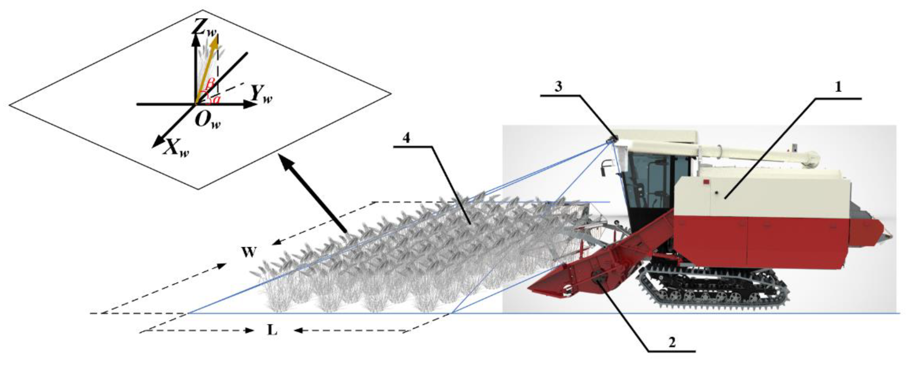
3.1. Wheat Lodging Direction Detection Model for Combine Harvesters Using Vehicle Vision

3.1.1. Model Construction

As shown in Figure 3, the vision system is constructed by installing a stereo camera at the front of the combine harvester with a certain angle for acquiring the images of the wheat to be harvested. For the impact of lodging on the direction of harvesting operations, we focused on studying the lodging direction parameter α on the horizontal projection plane of wheat in the field.
As shown in Figure 4, a static coordinate model in the dynamic environment of continuous harvesting operation is constructed according to the vision system. The left and right camera coordinate systems of the stereo camera are O c 1 X c 1 Y c 1 Z c 1 and O c 2 X c 2 Y c 2 Z c 2 , and O c 1 X c 1 Y c 1 Z c 1 is the camera’s basic coordinate system. The pixel coordinate systems constructed in images acquired with the left and right cameras are O o 1 U 1 V 1 and O o 2 U 2 V 2 . The image coordinate systems are O i 1 X i 1 Y i 1 and O i 2 X i 2 Y i 2 . The world coordinate system is O w X w Y w Z w . The X w and Y w axes of O w X w Y w Z w are on a horizontal plane. The Z w axis is vertically upward. The origins O w and O c 1 are on the same axis perpendicular to the horizontal plane with distance h .
The transformation of a point from A coordinate in the a coordinate system to the B coordinate in the b coordinate system can be expressed as B = H a b A . The H a b also represents the pose matrix of the b coordinate system in the a coordinate system. The coordinate of origin O i 1 for O i 1 X i 1 Y i 1 in O i 1 U i 1 V i 1 is ( u 01 , v 01 ) . The coordinate of origin O i 2 for O i 2 X i 2 Y i 2 in O o 2 U 2 V 2 is ( u 02 , v 02 ) . The single pixel size of the left and right camera sensor targets is consistent, in both length Δ x and width Δ y . According to Equation (20), H o 1 i 1 and H o 2 i 2 are calculated based on the affine transformation of scaling and translation.
H o 1 i 1 = [ Δ x 0 u 01 Δ x 0 Δ y v 01 Δ y 0 0 1 ] ,   H o 2 i 2 = [ Δ x 0 u 02 Δ x 0 Δ y v 02 Δ y 0 0 1 ]
The focal length of both the left and right cameras is f , and H i 1 c 1 and H i 2 c 2 are calculated based on pinhole imaging as follows:
H i 1 c 1 = z c 1 [ 1 f 0 0 0 1 f 0 0 0 1 0 0 0 ] ,   H i 2 c 2 = z c 2 [ 1 f 0 0 0 1 f 0 0 0 1 0 0 0 ]
The relative pose relationship between the left and right cameras is calculated based on the pose of the calibration board relative to the cameras within the coincident field of view of the cameras. R c 1 and R c 2 represent the rotational pose relationships between the cameras and the calibration board, respectively. T c 1 and T c 2 represent the translation pose relationships between the cameras and calibration board, respectively. The formula used to calculate H c 2 c 1 is as follows:
H c 2 c 1 = [ R T 0 1 ] , R = R c 2 R c 1 1 ,   Τ = T c 2 R T c 1
According to the pose relationship between O c 1 X c 1 Y c 1 Z c 1 and O w X w Y w Z w , the transformation H c 1 w between the camera coordinate system and the world coordinate system is calculated. O w X w Y w Z w is translated to O c 1 and rotated 90 + θ 1 ( 0 < θ 1 < 90 ) around X w to obtain O c 1 X c 1 Y c 1 Z c 1 . There is no scaling relationship between O c 1 X c 1 Y c 1 Z c 1 and O w X w Y w Z w . Therefore, H c 1 w can be calculated based on Equation (23).
H c 1 w = [ R T 0 1 ] ,   T = ( 0 , 0 , h )
The rotation matrix R is calculated as the left multiplication of a single rotation matrix based on the right-handed coordinate system [37]:
R = [ 1 0 0 0 cos ( 90 + θ 1 ) sin ( 90 + θ 1 ) 0 sin ( 90 + θ 1 ) cos ( 90 + θ 1 ) ]

3.1.2. IPM and Correction

The basic equation of IPM is constructed based on the coordinate relationship chains H o 1 i 1 , H i 1 c 1 and H c 1 w . The basic equation is corrected using the coordinate relationship chains H c 1 c 2 , H o 2 i 2 and H i 2 c 2 to improve the accuracy and reliability of the IPM model. The IPM is used for the calculation of the corresponding spatial top view in the world coordinate system based on the original image obtained with a sensor [38]. Therefore, the IPM equations for the left and right cameras can be constructed based on Equations (25) and (26), respectively. The [ x w 1 i ,   y w 1 i ,   z w 1 i ] and [ x w 2 i ,   y w 2 i ,   z w 2 i ] are the coordinates of the same spatial point P i obtained based on the coordinate relationship chains of the left and right cameras, respectively. [ u 1 i ,   v 1 i ] and [ u 2 i ,   v 2 i ] are the pixel coordinates of points p 1 i and p 2 i on the left and right images mapped from spatial point P i , which can be obtained from the images. The parameters Δ x , Δ y , f , u 01 , v 01 , u 02 , and v 02 can be obtained with camera calibration. The parameters h and θ 1 can be obtained using a ruler and angle measuring instrument.
[ x w 1 i y w 1 i z w 1 i 1 ] 4 × 1 = H o 1 w [ u 1 i v 1 i 1 ] 3 × 1 = H c 1 w H i 1 c 1 H o 1 i 1 [ u 1 i v 1 i 1 ] 3 × 1 = z c 1 [ R T 0 1 ] 4 × 4 [ 1 f 0 0 0 1 f 0 0 0 1 0 0 0 ] 4 × 3 [ Δ x 0 u 01 Δ x 0 Δ y v 01 Δ y 0 0 1 ] 3 × 3 [ u 1 i v 1 i 1 ] 3 × 1
[ x w 2 i y w 2 i z w 2 i 1 ] 4 × 1 = H o 2 w [ u 2 i v 2 i 1 ] 3 × 1 = H c 1 w H c 2 c 1 H i 2 c 2 H o 2 i 2 [ u 2 i v 2 i 1 ] 3 × 1 = z c 2 [ R T 0 1 ] 4 × 4 [ 1 f 0 0 0 1 f 0 0 0 1 0 0 0 ] 4 × 3 [ Δ x 0 u 02 Δ x 0 Δ y v 02 Δ y 0 0 1 ] 3 × 3 [ u 2 i v 2 i 1 ] 3 × 1
The coordinate transformation of the left camera is used as the basic equation of the IPM. The IPM is corrected using the deviation [ x w 1 i x w 2 i ,   y w 1 i y w 2 i ] between the coordinates [ x w 2 i ,   y w 2 i ] obtained from the IPM equation of the right camera and the coordinates [ x w 1 i ,   y w 1 i ] obtained from the basic equation. According to Equations (27) and (28), the correction is determined using the gross error elimination method, where n is the number of spatial points used for the IPM. There are calculation errors of the same spatial point coordinate, so the threshold ( x t , y t ) for gross error elimination can be calculated based on the mean ( Δ x ¯ ,   Δ y ¯ ) of the coordinate deviation. According to Equations (29) and (30), the corrected IPM coordinates ( x w i , y w i ) are calculated.
x w i = { x w 1 i , x w 1 i x w 2 i > x t x w 1 i x w 2 i 2 , x w 1 i x w 2 i x t ,   i = 1 , 2 , , n
y w i = { y w 1 i , y w 1 i y w 2 i > y t y w 1 i y w 2 i 2 , y w 1 i y w 2 i y t ,   i = 1 , 2 , , n
{ Δ x ¯ = i = 1 n x w i 1 x w i 2 n Δ y ¯ = i = 1 n y w i 1 y w i 2 n
{ x t = 2 i = 1 n ( x w i 1 x w i 2 ) Δ x ¯ n y t = 2 i = 1 n ( y w i 1 y w i 2 ) Δ y ¯ n

3.2. Dataset Constructed Using Adaptive Image Grid Division

3.2.1. The Local Region of Interest (ROI) for Wheat Lodging Direction Detection

The wheat lodging direction detection in the field is mainly used for the real-time operation control of harvesters, so the region of interest for detection is within a certain range of the front of the harvester. The length L d of the ROI is set based on the operating speed of the harvester. The maximum width of the harvester operation area does not exceed the full cutting width, so the width of the ROI is calculated as W d = W g + d , where W g is the header width and d is the margin.
As shown in Figure 5, the edges for the front and right of the header are extracted for fitting the lines l 11 and l 12 using the Hough transform. The intersection point p 11 between l 11 and the left edge of the image is calculated. A line l 13 parallel to U 1 of the image coordinate system is constructed based on p 11 . The intersection point p 12 between l 12 and l 13 is calculated. Along l 13 , p 12 is moved by d to obtain point p 13 . Along the opposite direction to V 1 in the left edge of the image, p 11 is moved by L d to obtain point p 14 . Based on points p 11 , p 13 and p 14 , a rectangle on the sides parallel to V 1 and U 1 is defined as the ROI for the wheat lodging direction detection.

3.2.2. Adaptive Image Grid Division Based on PM and IPM

The IPM can reduce the effect of the near-big–far-small phenomenon on detection, but the resolution of the transformed image will decrease. Therefore, using the original image as a data source for lodging direction detection, we performed non-uniform adaptive grid division on the original image using the PM and IPM of key points to establish the actual spatial area corresponding to each region equal after division. Firstly, according to Equations (27) and (28), the points P 1 and P 4 in the real 3D space corresponding to points p 11 and p 14 of the ROI for wheat lodging direction detection are calculated. Here, ( x w 1 , y w 1 ) and ( x w 4 , y w 4 ) represent the top view coordinates of P 1 and P 4 calculated using the IPM. According to the distance between P 1 and P 4 on the X w of O w X w Y w Z w , the ROI is evenly divided by m x , and the coordinates ( x d i , y d i ) of key points P d i for dividing are calculated based on Equation (31).
{ x d i = x w 1 i ( x w 1 x w 4 ) m x y d i = 0 ,   i = 0 , 2 , , m x
According to the inverse transformation of Equations (27) and (28), the image points p 1 d i corresponding to P d i are calculated. The ROI in the image is divided unevenly on the V 1 axis based on p 1 d i calculated using the IPM and PM, and evenly divided on the U 1 axis with the m y set based on experience to obtain small regions for the local direction detection of wheat lodging.

3.2.3. Dataset Construction

In this paper, image classification is applied to detect wheat lodging direction. The lodging directions are divided into eight classes. Starting from the positive direction of the x-axis and rotating counterclockwise, each direction label is defined as 1, 2, …, 8, respectively. The images of wheat lodging in these eight directions in the field are collected, with 10 images per group and a total of 80 images from these eight directions. As shown in Figure 5, the ROI with the wheat to be tested in the original image is divided into adaptive grids with an equal actual spatial area, and m x × m y small regions are obtained from a single image. Then, based on image preprocessing on small regions, such as noise addition, rotation, and scale transformation, the dataset is expanded by n r times to obtain a dataset of wheat lodging directions composed of 80 × m x × m y × n r image blocks, as shown in Figure 6.

3.3. The Construction of the BOVW Based on the Improved K-Means Algorithm

The i th region of an image is I i = { I i 1 , I i 2 , , I i e , , I i g } and the dataset to be classified constructed with adaptive image grid division is R = { r 1 , r 2 , , r i , , r m } . The improved k-means algorithm is used to classify R and construct a BOVW for wheat lodging detection.
  • Image feature point extraction based on SIFT
The feature points in each region of R are extracted based on the SIFT. The SIFT has good robustness to adapt scaling, rotation, translation, affine transformation, and noise. It includes four steps: (1) constructing scale space and detecting candidate feature points; (2) correcting; (3) purifying feature points; and (4) determining feature point direction parameters and constructing the feature vector.
The scale space is constructed based on the difference in the Gaussian function (DOG):
D ( x , y , σ ) = ( G ( x , y , k σ ) G ( x , y , σ ) ) × R ( x , y )
G ( x , y , σ ) is the Gaussian function:
G ( x , y , σ ) = 1 2 π σ 2 e x 2 + y 2 2 σ 2
G ( x , y , k σ ) G ( x , y , σ ) can be calculated as follows:
σ 2 G = G σ G ( x , y , k σ ) G ( x , y , σ ) k σ σ
The regional extreme points on the constructed scale space are detected as candidate feature points. For improving the contrast of the feature points and removing unstable edge points, the sub-pixel interpolation method is used to filter and remove candidate feature points with low contrast, and the edge points are recognized and removed according to the principal curvature value. The Taylor expansion of DOG is calculated as follows:
D ( X ) = D ( X 0 ) 2 D 2 X X + 1 2 X T 2 D 2 X X
The X = ( x , y , σ ) is discrete extreme points in scale space. The extreme points X ^ solved are as follows:
X ^ = 2 D 1 2 X 2 D X
Placing X ^ into Equation (35), we have
D ( X ^ ) = D + 1 2 D T X X ^
Based on | D ( X ^ ) | , the candidate feature points are selected. If | D ( X ^ ) | < φ , the corresponding candidate feature point has low contrast and is removed. To calculate the principal curvature of candidate feature points, a Hessian matrix is constructed as follows:
H ( x , y ) = [ h x x   h x y h x y   h y y ]
The maximum and minimum eigenvalues of matrix H are λ max and λ min , respectively. Considering the trace t r ( H ) = λ max + λ min and the determinant d e t ( H ) = λ max λ min of matrix H ,
t r 2 ( H ) det ( H ) = ( λ max + λ min ) 2 λ max λ min = ( γ + 1 ) 2 γ
where γ = λ max / λ min . To detect whether the principal curvature is less than the threshold value γ , it is only necessary to use Equation (40). When the principal curvature of candidate feature points exceeds a certain threshold, they are judged as edge points and removed.
t r 2 ( H ) det ( H ) > ( γ + 1 ) 2 γ
The feature point direction parameters are determined using the gradient directions. The gradient direction corresponding to the peak of the gradient direction histogram, calculated within the neighborhood of the feature point, is the main direction of the feature point. Additionally, the secondary peak value greater than 80% of the main peak value is used as the secondary direction of this feature point. The neighborhood of 16 × 16 feature points is divided into 16 regions of 4 × 4 , and the histogram of each region in eight gradient directions is calculated to construct a 128-dimensional feature vector for each feature point in the regions. For multichannel regions (RGB-D) obtained with the stereo camera, the 128-dimensional feature vectors of the feature points in each channel are calculated, and each feature point corresponds to four 128-dimensional feature vectors:
T i = ( T i 1 , T i 2 , T i 3 , T i 4 )
The feature vector of the feature point x i in the image channel I e is T i e = ( t i e 1 , t i e 2 , , t i e p , , t i e 128 ) .
2.
BOVW construction
Since the number of words in the BOVW is uncertain before clustering, the optimal number of clustering classes k m is determined using the weighted cluster validity evaluation function constructed based on the measuring parameters among classes in k-means clustering. The k initial clustering centers are selected based on the maximum and minimum distances, and the distance calculations are simplified using triangle inequality. All the feature points represented by the multichannel and multidimensional feature vectors T i e in the direction dataset are clustered to obtain the clustering classes centered on C = { c 1 , c 2 , , c k } . The center c j of each class is used as a visual word to construct the BOVW.

3.4. Local Direction Detection of Wheat Lodging

Each region of the image is analyzed based on BOVW. The frequencies of words appearing in the region r i are calculated to construct the region feature vector W i = ( w i 1 , w i 2 , , w i k m ) .
Since the feature vector W i of the dataset R is not linearly separable, the support-vector machine (SVM) is used. The feature space of W i is transformed into a space of higher dimension so that the features become linearly separable. In addition, a spatial pyramid is used based on a bag to reduce the loss of spatial information of the image represented using the BOVW. For the image resolution and wheat size, the image is divided into a layers. From the bottom to the top, there are patches of size 2 a 1 × 2 a 1 , 2 a 2 × 2 a 2 , , 1 and k × ( 2 a 1 × 2 a 1 + 2 a 2 × 2 a 2 + + 1 ) word frequencies for each image.
To avoid the curse of dimensionality for SVM, it is not the features but a kernel that is transformed. The histogram intersection kernel is adopted to transform the feature space into a higher dimension. The margin is defined as the closest distance between the separating hyperplane and any training sample. The separating hypersurface for two classes is constructed with SVM such that the margin between the two classes becomes as large as possible. To extend the SVM to a multiclass problem of wheat lodging direction detection, each class is compared with the rest of the training data, and then the class with the maximum distance to the hypersurface is selected. The classes of regions in the image are the wheat lodging directions in the regions, and all the directions in these regions are used to generate a lodging distribution map.

4. Results

4.1. Experimental Platform

To verify the effectiveness and advantages of the proposed method, the wheat lodging direction detection module was installed on a 4LZ-6A multifunctional intelligent crawler-type combine harvester developed by our team [39], as shown in Figure 7. The combine harvester is equipped with an intelligent control module, including a JCMC-54A controller, a controller area network (CAN) module, a motor driver, and an electric hydraulic pressure pusher. The control module works together with the detection module to achieve the intelligent operation of the harvester. The camera was ZED 2I with 110° (H) × 70° (V) × 120° (D) field of view, 2.1 mm focal length, 0.3 m–20 m depth range, and 5.07% TV distortion. The processor was a MIC-7700 industrial computer with i7-6700 CPU, DDR4-8G memory, Windows 10 system, Python 3.8.5 compilation environment, and Opencv 4.5.3. The software for the detection module was equipped with a warning function. When the camera could not acquire an image, the images acquired from three consecutive frames were the same, the images were all black, the calculation time was a timeout, and the results could not be sent to the control terminal, a warning would be triggered and displayed on the display screen. The experiments were conducted in wheat fields in Shiyezhou in Zhenjiang City, the Daizhuang Organic Agriculture Professional Cooperative in Jurong City, and the Wujiang National Modern Agriculture Demonstration Zone in Suzhou City. The results obtained from the wheat lodging direction detection module were sent to the control module using CAN, which provides data support for the automatic control of the overall movement, pose adjustment, and the adjustment of component parameters such as the header, reel, and lifting guard in the harvester. The harvester achieves safe and accurate intelligent operation by intelligently adjusting the operating parameters. The experiment was conducted in May, and the data collection time was 9:30 a.m.–16:30 p.m. during the harvesting period. The illumination on both cloudy and sunny days met the requirements for image acquisition (Figure 8).

4.2. Experimental Methods

Based on the images collected in the field, comparative experiments were conducted using the wheat lodging direction detection methods, namely the single-level word frequencies with existing k-means algorithm (SWF-EK), the single-level word frequencies with improved k-means (SWF-IK), and the pyramid word frequencies with improved k-means (PWF-IK). The effectiveness and advantages of the proposed method were verified in the field experiments.

4.2.1. The Experiment Method for the Comparison of BOVW Construction Methods

The images of wheat lodging in the eight directions in the field were collected, with 10 images per group. Based on an average of 100 grids per image, there were a total of 1000 regions in each direction. The 300 regions with obvious, slightly obvious, and indistinct direction information were selected from 1000 regions. Then, the dataset with 2700 regions for eight lodging directions and one non-lodging direction was obtained. Then, 70% of the dataset was used for training and 30% for testing; thus, each class in the training set contained 210 regions, and each class in the testing set contained 90 regions. This dataset was used for the comparison experiments of BOVW construction methods with SWF-EK, SWF-IK, and PWF-IK. The labels marked manually were used as truth values, and the evaluation indicators were calculated using Equations (42) and (43). TP is the true-positive value in the confusion matrix for network evaluation, FP is the false-positive value, FN is the false-negative value, and FPPI is the false-positive value per image [40].
p r e c i s i o n = T P T P + F P
r e c a l l = T P T P + F N

4.2.2. The Experiment Method for the Comparison of Wheat Lodging Direction Detection Methods

In the field, five experiments were conducted in five different fields with a speed of 1 m/s, a header height of 200 mm, a detection beat of 2 s, and an experimental distance of 20 m each time. For the experiment, 10 data were obtained each time, resulting in 50 data in total. Within the selected experimental fields, wheat had different lodging directions (Figure 9). The truth values of the lodging directions were measured and recorded manually in the field. The multiple directions for wheat growth within a region were measured, and the direction with the highest frequency of occurrence was used as the lodging direction of the region.
The detection accuracy of a region in an image was calculated by comparing the detected values and the true values within the region. The direction detection accuracy A i of an image was calculated based on the detection accuracy of the region, as shown in Equation (44). Here, m x i × m y i is the total number of the grid regions after dividing the i th image, and p i is the total number of regions with the correct detection of lodging direction in the i th image.
A i = p i m x i × m y i

4.3. Experimental Results and Discussion

4.3.1. Experiment Results for the Comparison of BOVW Construction Methods

The features of 2700 regions with different directions were extracted to construct a feature set. The existing and improved k-means algorithms were used to construct the BOVW, respectively, and the single image and a pyramid with weighted layers were used to extract the word frequency histograms of the image in the experiments. According to the image resolution and wheat size, the image was divided into a = 4 layers. From the bottom to the top, there were patches of size 8 × 8 , 4 × 4 , 2 × 2 , 1 . Using the 310 optimal centers obtained after clustering with improved k-means, there were 310 × 85 = 26350 word frequencies for each image.
For the limitations of using word frequencies as the detection indicator in a region, the word frequencies of 2700 regions were collected for the result analysis of expression using the BOVW. The word frequency histograms of 300 regions in each class were constructed, and the mean word frequencies of 300 regions were calculated for analyzing the differences in the dictionary expression among the different classes, as shown in Figure 10 and Figure 11.
From Figure 10 and Figure 11, we can see that, compared with the existing k-means algorithm, the BOVW constructed using the improved k-means more easily represented distinctive features of wheat lodging direction in the images. Compared with single-level word frequencies, the pyramid word frequencies could better reflect the detailed features of the image, reducing the loss of spatial information caused by word frequency histograms. Compared with other methods, the proposed PWF-IK could more accurately represent wheat lodging direction information.
The 810 regions in the test set were used in the experiments of wheat lodging direction classification based on SWF-EK, SWF-IK, and PWF-IK. Then, the confusion matrices were calculated, as shown in Figure 12.
According to the confusion matrices and evaluation indicators (42)–(43), the average precision (AP) and average recall (AR) were calculated for evaluating the performance of the different methods, as shown in Table 1 and Table 2.
From Table 1 and Table 2, we can see that, compared with SWF-EK and SWF-IK, the mAPs of the PWF-IK method increased by 6.53% and 6.89%, respectively, and the mARs increased by 6.55% and 6.92%, respectively. Compared with the existing k-means algorithm, the improved k-means had a significant impact on the improvements in mAP and mAR, both exceeding 6.53%. Compared with the single-level word frequencies, the pyramid word frequencies had a minor impact on the improvements in mAP and mAR, both exceeding 0.36%. The improved k-means and pyramid word frequencies can greatly assist in improving the accuracy of wheat lodging direction detection.

4.3.2. Experiment Results for the Comparison of Wheat Lodging Direction Detection Methods

The partial results of the five experiments for wheat lodging direction detection are shown in Figure 13, with one image in a group. In this figure, red represents the regions with incorrect direction detection, while green represents the regions with correct direction detection. From Figure 13, we can see that the detection accuracy was affected by the image quality. Compared with the field closer to the camera, the field farther away from the camera corresponded to a smaller region in the image, and there were fewer features of wheat for lodging direction detection. For the same object distance, when the region contained wheat with multiple directions, it was more prone to false-positive results. Compared with the existing k-means algorithm, the detection accuracy of wheat lodging direction for an image based on the improved k-means was higher. For small regions, the detection accuracy based on the pyramid word frequencies was higher than that based on single-level word frequencies. The proposed method had higher accuracy and better robustness in the lodging direction detection of wheat with dense growth and overlapped organs with images obtained from a tilted camera.
Based on the dataset constructed using adaptive image grid division, SWF-EK, SWF-IK, and PWF-IK were used for the field experiments of wheat lodging direction detection, and the A i values of 50 experiments of five groups were calculated. From Figure 14, we can see that the average A i values using SWF-EK, SWF-IK, and PWF-IK were 90.57%, 96.17%, and 97.28%, respectively. Compared with the SWF-EK and SWF-IK methods, the average A i values using the proposed PWF-IK method increased by 6.71% and 1.11%, respectively. The average time of wheat lodging direction detection for an image using SWF-EK, SWF-IK, and PWF-IK were 0.92 s, 0.98 s, and 1.16 s, respectively. Compared with the SWF-EK and SWF-IK methods, the average time using the proposed PWF-IK method increased by 0.24 s and 0.18 s, respectively. Although the improved k-means algorithm in this paper increased computational complexity, the calculation time had not significantly increased by using triangle inequality to simplify the distance calculations. The detection time of the proposed PWF-IK method was within the rhythm range of harvester operation control, meeting the closed-loop control requirements of intelligent operation for harvesters in the field.

5. Discussion and Conclusions

Due to the inconsistent lodging of wheat with dense growth and overlapped organs, it is difficult to detect lodging direction accurately and quickly using vehicle vision for combine harvesters based on the existing k-means algorithm with random initial centers and experiential number of classes. Therefore, in this paper, we improved the k-means algorithm based on a cluster validity evaluation function and a multichannel and multidimensional feature vector and proposed a local direction detection method of wheat lodging based on the BOVW. The following conclusions can be drawn:
(1) The k-means algorithm is improved by designing a cluster validity evaluation function to determine the optimal number of classes, adopting the maximum and minimum distances to select the initial clustering centers, constructing a multichannel and multidimensional feature vector to represent data, and using triangle inequality to simplify the distance calculations. It overcomes the challenges in achieving a level of clustering accuracy and efficiency in the existing k-means algorithm that do not easily meet the requirements for the detection of wheat lodging direction using vehicle vision due to the experiential number of classes, random initial clustering centers, limited features, and redundant distance calculations.
(2) A dataset construction method based on vehicle vision and adaptive image grid division is proposed. The basic equation of IPM is corrected using the coordinate relationship chain. The non-uniform adaptive grid division on the original image is performed based on the PM and IPM. It can extract regions with an equal actual area in the image for constructing a dataset of wheat lodging directions without being affected by the near-big–far-small phenomenon in the original image and low-resolution images after using the IPM.
(3) The BOVW is constructed using the improved k-means algorithm and direction dataset. The SIFT, PWF, HIK, and SVM methods are adopted and combined to construct a detection method of wheat lodging direction for combine harvesters. It reduces the loss of spatial information in the image represented using the BOVW and improves detection accuracy and efficiency.
(4) The proposed detection method of wheat lodging direction was used in a 4LZ-6A multifunctional intelligent crawler-type combine harvester developed by our team for comparative experiments. Compared with the SWF-EK and SWF-IK methods, the mAPs of local direction detection for the wheat lodging using the proposed PWF-IK method increased by 6.53% and 6.89%, respectively, and the mARs increased by 6.55% and 6.92%, respectively. The average direction detection accuracy for the image using the proposed PWF-IK method increased by 6.71% and 1.11%, respectively. The average time of direction detection using the proposed method was 1.16 s. Compared with the SWF-EK and SWF-IK methods, the average time using the proposed PWF-IK method increased by 0.24 s and 0.18 s, respectively. Although the proposed PWF-IK method increased computational complexity, the calculation time had not significantly increased by using triangle inequality to simplify calculations, meeting the closed-loop control requirements of intelligent operation for harvesters in the field. The proposed method can accurately and rapidly detect wheat lodging direction for combine harvesters using vehicle vision and can further implement the closed-loop control of intelligent harvesting operation.
The method proposed in this paper is mainly used for wheat lodging detection in combine harvesters under natural light during the day. In the future, the proposed method can be further used for the lodging detection of different field crops, such as rice, rape, and corn, in the harvesting machinery. Additionally, the detection environment can be extended from day to night with a light source. It can provide data support for the automatic control of the overall movement, pose adjustment, and adjustment of component parameters, such as the header, reel, and lifting guard, in the harvester. It can lay a theoretical foundation for achieving the leap of domestic harvesting machinery from low end to high end and has important practical significance for the intelligent operation of harvesting equipment and the implementation of precision agriculture.

Author Contributions

Conceptualization, Q.Z., L.X. and X.X.; data curation, Q.C. and Z.L.; formal analysis, Q.Z.; funding acquisition, Q.Z. and L.X.; investigation, Q.C.; methodology, Q.Z. and Q.C.; project administration, Q.Z. and Z.L.; resources, Q.Z.; software, Q.Z. and Q.C.; supervision, L.X. and X.X.; validation, Q.C. and Z.L.; visualization, Q.Z.; writing—original draft preparation, Q.Z. and L.X.; writing—review and editing, Q.Z. All authors have read and agreed to the published version of the manuscript.

Funding

This research was funded by a Project Funded by the Priority Academic Program Development of Jiangsu Higher Education Institutions, grant number PAPD-2018-87; the Shandong Provincial Postdoctoral Innovation Project, grant number SDCX-ZG-202203051; the Jiangsu Province Higher Education Basic Science (Natural Science) Research Project, grant number 23KJB210006; and the Zhenjiang Key R&D Plan (Industry Foresight and Common Key Technology), grant number GY2023001.

Data Availability Statement

Not applicable.

Conflicts of Interest

The authors declare no conflict of interest.

References

  1. Jiang, S.; Hao, J.; Li, H.; Zuo, C.; Geng, X.; Sun, X. Monitoring wheat lodging at various growth stages. Sensors 2022, 22, 6967. [Google Scholar] [CrossRef]
  2. Yang, S.; Wang, P.; Wang, S.; Tang, Y.; Ning, J.; Xi, Y. Detection of wheat lodging in UAV remote sensing images based on multi-head self-attention DeepLab v3+. Trans. Chin. Soc. Agric. Mach. 2022, 53, 213–219, 239. [Google Scholar]
  3. Wen, J.; Yin, Y.; Zhang, Y.; Pan, Z.; Fan, Y. Detection of wheat lodging by binocular cameras during harvesting operation. Agriculture 2023, 13, 120. [Google Scholar] [CrossRef]
  4. Chauhan, S.; Darvishzadeh, R.; Boschetti, M.; Pepe, M.; Nelson, A. Remote sensing-based crop lodging assessment: Current status and perspectives. ISPRS J. Photogramm. Remote Sens. 2019, 151, 124–140. [Google Scholar] [CrossRef]
  5. Chen, Y.; Sun, L.; Pei, Z.; Sun, J.; Li, H.; Jiao, W.; You, J. A simple and robust spectral index for identifying lodged maize using Gaofen1 satellite data. Sensors 2022, 22, 989. [Google Scholar] [CrossRef]
  6. Guan, H.; Huang, J.; Li, L.; Li, X.; Ma, Y.; Niu, Q.; Huang, H. A novel approach to estimate maize lodging area with PolSAR data. IEEE Trans. Geosci. Remote Sens. 2022, 60, 1–17. [Google Scholar] [CrossRef]
  7. Han, L.; Yang, G.; Yang, X.; Song, X.; Xu, B.; Li, Z.; Wu, J.; Yang, H.; Wu, J. An explainable XGBoost model improved by SMOTE-ENN technique for maize lodging detection based on multi-source unmanned aerial vehicle images. Comput. Electron. Agric. 2022, 194, 106804. [Google Scholar] [CrossRef]
  8. Kang, G.; Wang, J.; Zeng, F.; Cai, Y.; Kang, G.; Yue, X. Lightweight detection system with global attention network (GloAN) for rice lodging. Plants 2023, 12, 1595. [Google Scholar] [CrossRef]
  9. Dai, X.; Chen, S.; Jia, K.; Jiang, H.; Sun, Y.; Li, D.; Zheng, Q.; Huang, J. A decision-tree approach to identifying paddy rice lodging with multiple pieces of polarization information derived from Sentinel-1. Remote Sens. 2023, 15, 240. [Google Scholar] [CrossRef]
  10. Murakami, T.; Yui, M.; Amaha, K. Canopy height measurement by photogrammetric analysis of aerial images: Application to buckwheat (Fagopyrum esculentum Moench) lodging evaluation. Comput. Electron. Agric. 2012, 89, 70–75. [Google Scholar] [CrossRef]
  11. Han, D.; Yang, H.; Yang, G.; Qiu, C. Monitoring model of corn lodging based on Sentinel-1 radar image. In 2017 SAR in Big Data Era: Models, Methods and Applications (BIGSARDATA); IEEE: Piscataway, NJ, USA, 2017. [Google Scholar]
  12. Liu, T.; Li, R.; Zhong, X.; Jiang, M.; Jin, X.; Zhou, P.; Liu, S.; Sun, C.; Guo, W. Estimates of rice lodging using indices derived from UAV visible and thermal infrared images. Agric. For. Meteorol. 2018, 252, 144–154. [Google Scholar] [CrossRef]
  13. Zhao, X.; Yuan, Y.; Song, M.; Ding, Y.; Lin, F.; Liang, D.; Zhang, D. Use of unmanned aerial vehicle imagery and deep learning UNet to extract rice lodging. Sensors 2019, 19, 3859. [Google Scholar] [CrossRef] [PubMed]
  14. Wan, L.; Du, X.; Chen, S.; Yu, F.; Zhu, J.; Xu, T.; He, Y.; Cen, H. Rice panicle phenotyping using UAV-based multi-source spectral image data fusion. Trans. Chin. Soc. Agric. Eng. 2022, 38, 162–170. [Google Scholar]
  15. Xie, B.; Wang, J.; Jiang, H.; Zhao, S.; Liu, J.; Jin, Y.; Li, Y. Multi-feature detection of in-field grain lodging for adaptive low-loss control of combine harvesters. Comput. Electron. Agric. 2023, 208, 107772. [Google Scholar] [CrossRef]
  16. Chauhan, S.; Darvishzadeh, R.; Boschetti, M.; Nelson, A. Discriminant analysis for lodging severity classification in wheat using RADARSAT-2 and Sentinel-1 data. ISPRS J. Photogramm. Remote Sens. 2020, 164, 138–151. [Google Scholar] [CrossRef]
  17. Chauhan, S.; Darvishzadeh, R.; Boschetti, M.; Nelson, A. Estimation of crop angle of inclination for lodged wheat using multi-sensor SAR data. Remote Sens. Environ. 2020, 236, 111488. [Google Scholar] [CrossRef]
  18. Yu, J.; Cheng, T.; Cai, N.; Lin, F.; Zhou, X.; Du, S.; Zhang, D.; Zhang, G.; Liang, D. Wheat lodging extraction using Improved_Unet network. Front. Plant Sci. 2022, 13, 1009835. [Google Scholar] [CrossRef]
  19. Biswal, S.; Chatterjee, C.; Mailapalli, D.R. Damage assessment due to wheat lodging using UAV-based multispectral and thermal imageries. J. Indian Soc. Remote Sens. 2023, 51, 935–948. [Google Scholar] [CrossRef]
  20. Hu, X.; Gu, X.; Sun, Q.; Yang, Y.; Qu, X.; Yang, X.; Guo, R. Comparison of the performance of multi-source three-dimensional structural data in the application of monitoring maize lodging. Comput. Electron. Agric. 2023, 208, 107782. [Google Scholar] [CrossRef]
  21. Cao, W.; Qiao, Z.; Gao, Z.; Lu, S.; Tian, F. Use of unmanned aerial vehicle imagery and a hybrid algorithm combining a watershed algorithm and adaptive threshold segmentation to extract wheat lodging. Phys. Chem. Earth 2021, 123, 103016. [Google Scholar] [CrossRef]
  22. Sun, Q.; Chen, L.; Xu, X.; Gu, X.; Hu, X.; Yang, F.; Pan, Y. A new comprehensive index for monitoring maize lodging severity using UAV-based multi-spectral imagery. Comput. Electron. Agric. 2022, 202, 107362. [Google Scholar] [CrossRef]
  23. Modi, R.U.; Chandel, A.K.; Chandel, N.S.; Dubey, K.; Subeesh, A.; Singh, A.K.; Jat, D.; Kancheti, M. State-of-the-art computer vision techniques for automated sugarcane lodging classification. Field Crops Res. 2023, 291, 108797. [Google Scholar] [CrossRef]
  24. Sun, J.; Zhou, J.; He, Y.; Jia, H.; Liang, Z. RL-DeepLabv3+: A lightweight rice lodging semantic segmentation model for unmanned rice harvester. Comput. Electron. Agric. 2023, 209, 107823. [Google Scholar] [CrossRef]
  25. Yu, J.; Cheng, T.; Cai, N.; Zhou, X.G.; Diao, Z.; Wang, T.; Du, S.; Liang, D.; Zhang, D. Wheat lodging segmentation based on Lstm_PSPNet deep learning network. Drones 2023, 7, 143. [Google Scholar] [CrossRef]
  26. Tang, Z.; Sun, Y.; Wan, G.; Zhang, K.; Shi, H.; Zhao, Y.; Chen, S.; Zhang, X. Winter wheat lodging area extraction using deep learning with GaoFen-2 satellite imagery. Remote Sens. 2022, 14, 4887. [Google Scholar] [CrossRef]
  27. Huang, X.; Xuan, F.; Dong, Y.; Su, W.; Wang, X.; Huang, J.; Li, X.; Zeng, Y.; Miao, S.; Li, J. Identifying corn lodging in the mature period using Chinese GF-1 PMS images. Remote Sens. 2023, 15, 894. [Google Scholar] [CrossRef]
  28. Zhu, H.; Luo, C.; Guan, H.; Zhang, X.; Yang, J.; Song, M.; Liu, H. Object-oriented extraction of maize fallen area based on multi-source satellite remote sensing images. Remote Sens. Technol. Appl. 2022, 37, 599–607. [Google Scholar]
  29. Shu, M.; Bai, K.; Meng, L.; Yang, X.; Li, B.; Ma, Y. Assessing maize lodging severity using multitemporal UAV-based digital images. Eur. J. Agron. 2023, 144, 126754. [Google Scholar] [CrossRef]
  30. Yu, M.; Liu, X.J. Computer image content retrieval considering k-means clustering algorithm. Math. Probl. Eng. 2022, 2022, 7. [Google Scholar] [CrossRef]
  31. Singh, J.P.; Bouguila, N. Proportional data clustering using k-means algorithm: A comparison of different distances. In Proceedings of the IEEE International Conference on Industrial Technology (ICIT), Toronto, ON, Canada, 22–25 March 2017; IEEE: Piscataway, NJ, USA. [Google Scholar]
  32. Lin, J.T.; Peng, J.W. Adaptive inverse perspective mapping transformation method for ballasted railway based on differential edge detection and improved perspective mapping model. Digit. Signal Process. 2023, 135, 11. [Google Scholar] [CrossRef]
  33. Hu, M.; Tsang, E.C.C.; Guo, Y.; Zhang, Q. An improved k-means algorithm with spatial constraints for image segmentation. In Proceedings of the 20th International Conference on Machine Learning and Cybernetics (ICMLC), Adelaide, Australia, 4–5 December 2021. Electr Network. [Google Scholar]
  34. Yu, L.; Chang, Z.; Xue, S.; Quan, Z. Hyperspectral image classification algorithm based on entropy weighted K-means with global information. J. Image Graph. 2019, 24, 630–638. [Google Scholar]
  35. Xiaotian, M.; Yanlei, X.; Xindong, W.; Run, H.; Yuting, Z. Crop line detection based on improved k-means feature point clustering algorithm. J. Agric. Mech. Res. 2020, 42, 26–30. [Google Scholar]
  36. Chunhui, Z.; Ying, W.; Kaneko, M. Improved k-means clustering method for codebook generation. Chin. J. Sci. Instrum. 2012, 33, 2380–2386. [Google Scholar]
  37. Zhang, Q.; Gao, G.Q. Hand-eye calibration and grasping pose calculation with motion error compensation and vertical-component correction for 4-R(2-SS) parallel robot. Int. J. Adv. Robot. Syst. 2020, 17, 1729881420909012. [Google Scholar] [CrossRef]
  38. Luo, Y.; Wei, L.; Xu, L.; Zhang, Q.; Liu, J.; Cai, Q.; Zhang, W. Stereo-vision-based multi-crop harvesting edge detection for precise automatic steering of combine harvester. Biosyst. Eng. 2022, 215, 115–128. [Google Scholar] [CrossRef]
  39. Zhang, Q.; Hu, J.; Xu, L.; Cai, Q.; Yu, X.; Liu, P. Impurity/breakage assessment of vehicle-mounted dynamic rice grain flow on combine harvester based on improved Deeplabv3+ and YOLOv4. IEEE Access 2023, 11, 49273–49288. [Google Scholar] [CrossRef]
  40. Zhang, Q.; Gao, G. Prioritizing robotic grasping of stacked fruit clusters based on stalk location in RGB-D images. Comput. Electron. Agric. 2020, 172, 105359. [Google Scholar] [CrossRef]
Figure 1. Diagram of the improved k-means algorithm. X : the sample set; x ¯ : the center of X ; c j : the center of X j ; d ( x ¯ , c j ) : the distance between x ¯ and c j ; d ( x i , c j ) : the distance between x i and c j ; x i : the sample in X ; w i j : the membership in vector W i ; D q : the distance matrix; X 1 , X 2 , X k : the first, second, and k th sample subsets, respectively; k : the number of classes; k m : The optimal number of classes; c 01 , c q 1 : the centers of X 1 ; c 02 , c q 2 : the centers of X 2 ; c q k : the center of X k ; T 0 , T q : the feature vectors; J ( k ) 0 , J ( k ) q : the improved weighted cluster validity evaluation functions; D ( k ) 0 , D ( k ) q : the inter-class similarities; N ( k ) 0 , N ( k ) q : the intra-class similarities; μ 0 , μ q : the measure parameters among classes. The subscripts 0 and q represent the 0th and qth iterations, respectively. The areas enclosed by the blue lines are sample subsets. The green lines represent the calculated parameters of w i j . The orange lines represent d ( x i , c j ) . The red points represent the centers of sample subsets.
Agronomy 13 02227 g001
Figure 2. Improved k-means algorithm process.
Agronomy 13 02227 g002
Figure 3. The vision system for wheat lodging direction detection: 1: combine harvester; 2: header; 3: stereo camera; 4: wheat to be harvested.
Agronomy 13 02227 g003
Figure 4. The static coordinate model.
Agronomy 13 02227 g004
Figure 5. Dataset constructed with adaptive image grid division.
Agronomy 13 02227 g005
Figure 6. Dataset of wheat lodging directions: 0: non-lodging; 1–8: eight lodging directions.
Agronomy 13 02227 g006
Figure 7. Experimental platform.
Agronomy 13 02227 g007
Figure 8. Acquired images: (a) sunny day; (b) cloudy day.
Agronomy 13 02227 g008
Figure 9. Lodging directions of wheat: 0: non-lodging; 1–8: 8 lodging directions.
Agronomy 13 02227 g009
Figure 10. Word frequency histograms: (a) SWF-EK; (b) SWF-IK; (c) PWF-IK. 0: non-lodging; 1–8: eight lodging directions. The colors represent different regions.
Agronomy 13 02227 g010
Figure 11. Histograms of mean word frequencies: (a) SWF-EK; (b) SWF-IK; (c) PWF-IK. 0: non-lodging; 1–8: eight lodging directions.
Agronomy 13 02227 g011
Figure 12. Confusion matrices: (a) SWF-EK; (b) SWF-IK; (c) PWF-IK. The color depths represent the sizes of the values.
Agronomy 13 02227 g012
Figure 13. Local direction detection results of wheat lodging: (a) SWF-EK; (b) SWF-IK; (c) PWF-IK.
Agronomy 13 02227 g013
Figure 14. Direction detection accuracy.
Agronomy 13 02227 g014
Table 1. The results of AP.
Methods0
/%
1
/%
2
/%
3
/%
4
/%
5
/%
6
/%
7
/%
8
/%
mAP/%
SWF-EK93.6289.2590.7089.7789.5385.4287.6490.1195.4090.16
SWF-IK95.7496.7798.8497.8397.6794.7495.4095.5197.7396.69
PWF-IK95.7498.8998.8597.8397.7095.7495.4596.5596.7097.05
Table 2. The results of AR.
Methods0
/%
1
/%
2
/%
3
/%
4
/%
5
/%
6
/%
7
/%
8
/%
mAP/%
SWF-EK97.7892.2286.6787.7885.5691.1186.6791.1192.2290.12
SWF-IK10010094.4410093.3310092.2294.4495.5696.67
PWF-IK10098.8995.5610094.4410093.3393.3397.7897.04
Disclaimer/Publisher’s Note: The statements, opinions and data contained in all publications are solely those of the individual author(s) and contributor(s) and not of MDPI and/or the editor(s). MDPI and/or the editor(s) disclaim responsibility for any injury to people or property resulting from any ideas, methods, instructions or products referred to in the content.

