1. Introduction
Technological advancements have revolutionized the agricultural industry and have significantly improved agricultural practices. The use of information and communication technologies in agriculture is collectively referred to as smart or precision agriculture [
1]. Technology has been integrated into various domains of the agricultural ecosystem, and examples include automated irrigation systems that use sensors to monitor soil moisture levels and weather patterns [
2] and the use of robotics to perform tasks such as harvesting crops, planting seeds, and weeding fields [
3]. These technological innovations have increased efficiency, reduced labour costs, and minimized the impact of farming on the environment [
3].
Yield mapping is the other such example that has gained widespread adoption due to advancements in harvesting equipment. The combine harvester is equipped with a data acquisition system that enables the collection of crop yield data during the harvesting process, including location, grain flow, and area [
4]. Data from yield maps usually contain thousands of data points which have to be interpolated to create continuous yield maps that can be used for decision-making, diagnosing production issues, and optimizing management practices, as well as in research applications [
4].
Data from combines, however, often contain errors arising from systematic and operator actions. Previous research [
5,
6] has identified several of such errors, including yield map smoothing errors, unknown crop width entering the header during harvest, time lag of grain through the threshing mechanism, positional errors, surging grain through the combine transport system, and voids/holes. As yield is important for decision-making, it is important to devise a means to mitigate the negative effects of such errors. To this end, several approaches have been defined.
Numerous solutions have been proposed to address the spatial errors [
4,
7,
8], with some focused on a single error while others aimed to tackle multiple issues. Nonetheless, a solution for identifying and filtering voids/holes in yield maps remains yet to be defined. Voids typically result from topographical features such as waterlogging, rendering it impossible to till and consequently leaving no data points for such areas. Currently, interpolation is utilized to fill voids by incorporating neighbouring data points. However, this method is prone to errors as voids increase in size. Identifying voids in yield maps could significantly enhance the performance of downstream processes, such as interpolation.
The other limitation is that, currently, data quality of yield datasets in based the calculation of root mean square error after interpolation. This requires weighbridge data which can sometimes be unavailable, and in some cases unreliable [
9]. This can affect the quality of decisions made from such unreliable data. This paper proposes a mapping of spatial errors to form data quality dimensions (DQDs), which can be used to assess the quality of yield data without the need for a gold standard (weighbridge data). DQDs provide an acceptable way to measure data quality [
10]. DQDs have been used in many fields to standardise the description of quality errors so that quality improvements processes can be evaluated on a comparative basis [
11]. As data from multiple sources is increasingly being integrated for decision-making, mapping spatial errors to DQDs would allow for a unified data quality assessment framework that is based on similar metrics across multiple data sources.
This paper, therefore, implements a solution to achieve two main objectives, namely: (1) To develop a novel algorithm to identify voids in yield maps. This uses yield data (location and yield) and field boundary data. (2) Create a mapping of three spatial errors, including GPS errors, yield surges, and voids, to two common DQDs of accuracy and completeness. This allows the use of DQDs as a means to assess the quality of yield datasets without the need of a gold standard and also enable seamless integration with other IoT applications that are based on DQDs. Inverse distance weighting was used as an example, as it is one of the most common downstream process for yield map data.
The rest of the paper is structured as follows;
Section 2 provides an in-depth analysis of spatial errors commonly observed in yield datasets, including GPS errors, yield surges, and voids.
Section 3 outlines the approach to map data quality dimensions, specifically accuracy and completeness, to the spatial errors discussed in the preceding section.
Section 4 offers a detailed discussion of the novel void detection and correction algorithm. It also elucidates the mathematical implementation of the evaluation and data quality scoring strategies.
Section 5 presents the results obtained and extensively discusses their practical implications and potential applications. Finally, in
Section 6, a comprehensive summary and conclusion are presented.
2. Spatial Error Processing
Yield map datasets are a vital tool for site-specific and paddock management-based decision-making systems [
5,
6,
12]. These datasets, however, usually contain many errors arising from different sources. Previous research [
8] has identified several of these errors, including unknown crop width, the time lag of the grain, inappropriate GPS recording, yield surges, and voids. For the purposes of this research, only GPS errors, yield surges, and voids were considered. These are highlighted in the next section.
2.1. GPS Errors
This paper discusses two types of GPS errors: those occurring while the combine is stationary but still recording data because the header has not been lifted, and those arising from recording data outside the field boundary. To identify the first type of GPS error, the research employs an approach proposed by [
8], which uses Pythagoras’ theorem to calculate the distance between consecutive points. Any points with zero travel distance are deemed erroneous. For the second type of GPS error, field boundary data is used. Any points on the yield map that lie outside the field boundary are considered erroneous.
2.2. Yield Surges
Yield surges refers to the difference between the actual yield measurement and the measurements obtained from the combine. According to Beck et al. [
4], yield surges are rapid changes in indicated yield over a short distance, typically resulting from operator actions such as a sudden decrease in forward speed during a period of high grain flow [
4]. In contrast, Robinson et al. [
8] suggest a statistical method that utilizes a moving average mean and standard deviation to detect erroneous yield surges. However, this paper employs a distinct approach that uses absolute median deviation, as significant outliers can adversely affect the mean.
2.3. Voids Errors
Fields typically have areas or sections that cannot be planted due to their topographical features, such as waterlogging or hills, making them unsuitable for tilling. Therefore, farmers usually plant around such areas, resulting in the combine harvester not producing any data for those sections during harvesting, resulting in voids or holes in the yield map. Without GPS or yield data, these voids can be challenging to identify.
To generate contour maps and high-resolution yield maps, interpolation techniques are employed to fill the voids with nearby data points. However, the accuracy of the interpolation is impacted as the size of the void increases. Therefore, voids must be identified and treated as unique cases.
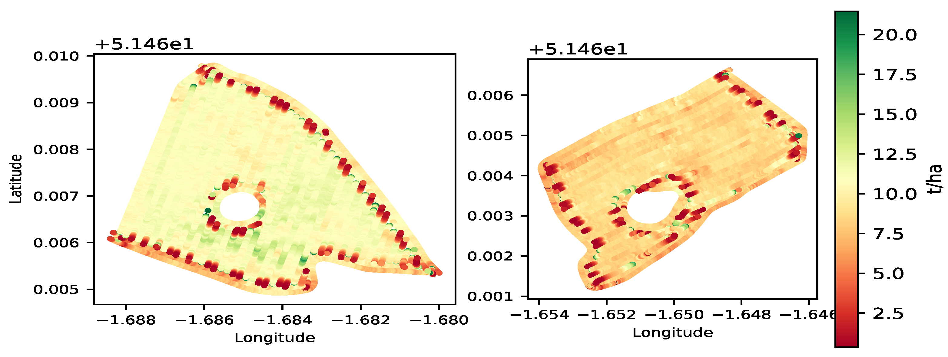
Figure 1 shows a yield map with a void, with the white portion in the centre representing the void. This paper introduces a novel approach for identifying and addressing voids, which is highlighted in
Section 4.1.
3. Data Quality Mapping
Data quality control for yield data is currently based on spatial errors. After spatial interpolation, the RMSE score is calculated as a quality indicator. If the score is small, this indicates good quality yield data. If the score is big, however, this means that the yield data is of poor quality. To calculate the RMSE score, interpolated values have to be compared to values from the weighbridge.
The data from the weighbridge, however, can suffer inaccuracies. This can be caused by several factors, including noise as the machine vibrates and errors from other foreign bodies that enter the system [
9]. Weighbridge data is not available for the vast majority of the fields. This leaves most fields without a reference point from which to evaluate yield quality and mapping, and, therefore, it is difficult to determine the trustworthiness of data used to make decisions. Establishing a quality score which can be determined independently from weighbridge data is imperative.
Moreover, as precision agriculture expands, different data sources and data types are being integrated and used simultaneously. Data are from weather stations, soil sensors, and many other IoT-based data collection methods. Data quality control for this kind of data is based on data quality dimensions, and indeed this is the standard for data quality assurance in IoT [
10]. Integrating quality assurance for yield datasets with other existing IoT sources to support organizational level decision-making that is based on quality data requires streamlining all quality assurance processes into a single pipeline that uses the same standard metrics.
Data quality dimensions offer a way to assess data quality using associated metrics likes accuracy and completeness. Previous research [
13] has built and tested an end-to-end data quality assessment framework that uses DQDs to assess data quality in real-time with no need for a gold standard (weighbridge data). This is ideal for cases where weighbridge data is not present, or has inaccuracies. This quality assurance process can also integrate with other IoT data sources for a holistic end-to-end data quality assessment.
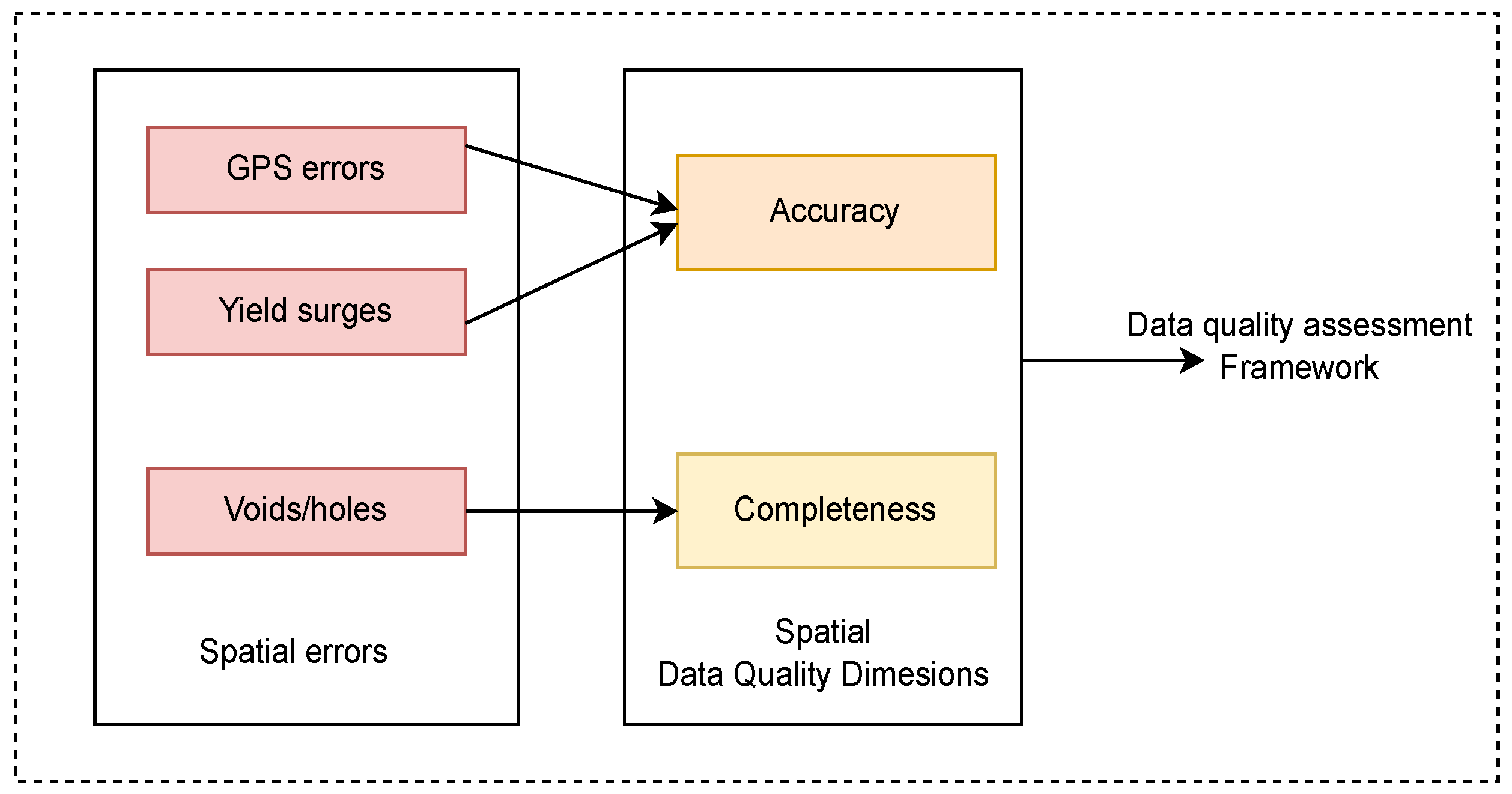
To achieve this, this paper creates a mapping between spatial errors and DQDs. The definitions of spatial errors and relationships between them are informed by previous research [
14]. The presence, or lack, of spatial errors leads to a deterministic change in quality evaluation metrics and RMSE. This relationship can be used to determine a quality score for the data, which can be used to assess the trustworthiness of the yield datasets and how much credence the data should be used for decision-making.
Figure 2 shows the mapping flow between spatial errors and DQDs.
3.1. Geospatial Data Quality Dimensions
The measure of quality is subjective and largely depends on the context in which it is applied. In manufacturing, for example, quality is often evaluated based on the product’s physical attributes [
14]. However, when it comes to data quality, it can be challenging to define as data lacks physical attributes. Instead, data quality is determined by intangible properties such as accuracy and completeness, which are collectively referred to as data quality dimensions (DQDs). Using DQDs provides an effective way to measure data quality, and several authors have proposed different DQDs and associated metrics to assess it [
10].
Unlike other datasets, geospatial data describe phenomena in multiple dimensions, including spatial, temporal, and thematic components [
14]. Therefore, DQDs for geospatial datasets have to be defined similarly. The paper defines spatial and thematic components for accuracy, while only the thematic component was used for completeness. This is due to the unavailability of time data for many farms. The mathematical definitions used here are informed by previous research in [
5,
8,
14].
3.1.1. Accuracy
Spatial accuracy (positional accuracy) is applied to the spatial component of a geospatial dataset. Metrics are well defined for point entities, but widely accepted metrics for lines and area are yet to be developed [
14]. We define area errors as the points (spatial coordinates that are outside a defined field of interest. These are inappropriate GPS recordings. There are two distinctions, which are points outside the field boundary and outlier points recorded while the machine is stationary.
where n is the number of points outside the defined boundary, and spatial error is the distance a given point is from the defined boundary. To define spatial errors, this paper used the same approach defined in [
8];
Thematic accuracy (or attribute accuracy) varies with a measurement scale. The attribute, in this case, is the yield. Beck et al. [
4] define this as yield surges. There have been other techniques that have been used to eliminate this kind of error. For example, ref. [
8] used a statistical identifier based on moving average mean and standard deviation. This paper uses median absolute deviation to filter out yield surges as the mean can be affected by outliers, Therefore:
where
is the number of outlier points in a given field, and
n is the total number of points in the field.
To calculate
, a statistical method that employs median absolute deviations (MAD) is utilized. Absolute deviation from the median has long been utilized to filter outliers [
15]. The median is a measure of central tendency, and is preferable to the mean as it is less susceptible to the presence of outliers, which can have a disproportionate impact. MAD was calculated using the formula defined by Huber et al. [
16].
where
is the original observations,
is the median of the series, and
is data normalization constant defined by [
17]. It is defined as
, where
is the 0.75 quantile of that underlying distribution. The normalisation step is important because otherwise MAD would estimate the scale up to a multiplicative constant [
16] only.
3.1.2. Completeness
Thematic completeness is based on voids/holes in the yield maps. Voids are a well-known problem that affects the quality of yield maps and, subsequently, the accuracy of any interpolation technique [
18,
19]. Currently, there is no defined method to identify and mitigate the effects of voids. Current approaches aim to fill voids. This affects not only the accuracy of the interpolation methods, but also downstream processes like yield prediction that might be based on such erroneous data. This paper implements a novel approach to identifying voids. This is discussed in
Section 4.1. Thematic completeness is therefore given by
where
is the number of grids that form the void and
n is total number of grids for a given yield map.
4. Implementation
The system implementation was divided into two stages. The initial stage involves identifying and classifying spatial errors. Three spatial errors were used in this implementation. The other stage involves mapping the defined spatial error to DQDs and assessing the impact of DQDs on the spatial interpolation. Spatial interpolation was used as an assessment example because its one of the most common pre-processing techniques used to construct usable yield maps [
20,
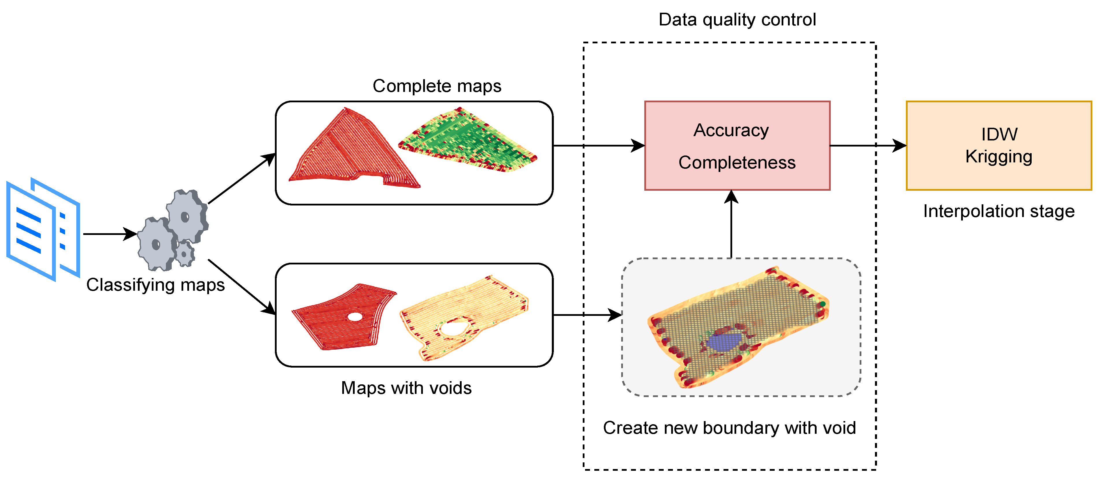
21]. Each of these stages is highlighted in detail in the following sections.
Figure 3 shows the end-to-end system flow of the implementation, showing void identification and correction in stage one and data quality mapping in stage two.
4.1. Void Error Correction
Yield map errors can be attributed to several causes. Prior research has identified some of these errors [
8]. This paper focuses on three types of errors, namely GPS errors, yield surges, and voids. Unlike GPS errors and yield surges, no established methods exist to identify yield maps with voids. Thus, this section presents a novel approach to detecting voids in yield maps.
Two inputs are required to interpolate yield maps spatially: yield map data consisting of GPS points with corresponding yield measurements, and field boundaries defined by a set of GPS points delineating the field’s limits. The latter is used to restrict the interpolation process to within the field.
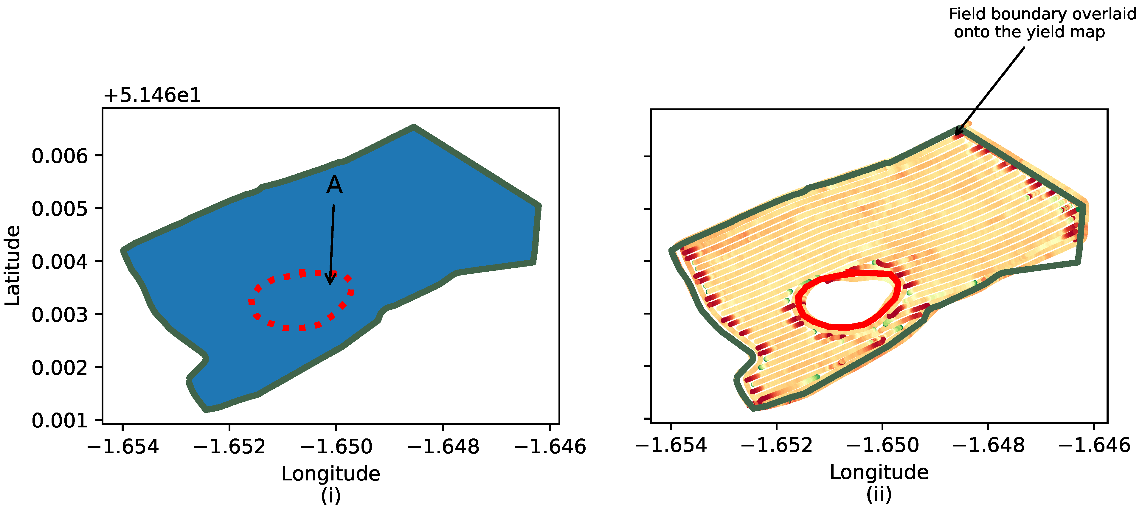
Figure 4 illustrates the importance of restricting yield map interpolation to the limits of the field, as shown by the green boundary line. Without such restriction, interpolation would continue indefinitely beyond the field boundary. When dealing with yield maps that contain voids, however, an additional inner boundary exists (artefact A) that is not accounted for in the original boundary file. As a result, interpolation will continue until the void is filled. This can significantly impact the accuracy of interpolation methods and downstream processes, such as yield prediction, that rely on such data. Therefore, it is crucial to identify yield maps with voids and reconstruct the boundary files to reflect these physical features.
Various approaches can help identify voids in yield maps, such as computer vision, image processing, and artificial-intelligence-based solutions, while these methods can achieve positive results, they face challenges such as the need for a considerable amount of data to train and test and high computational costs.
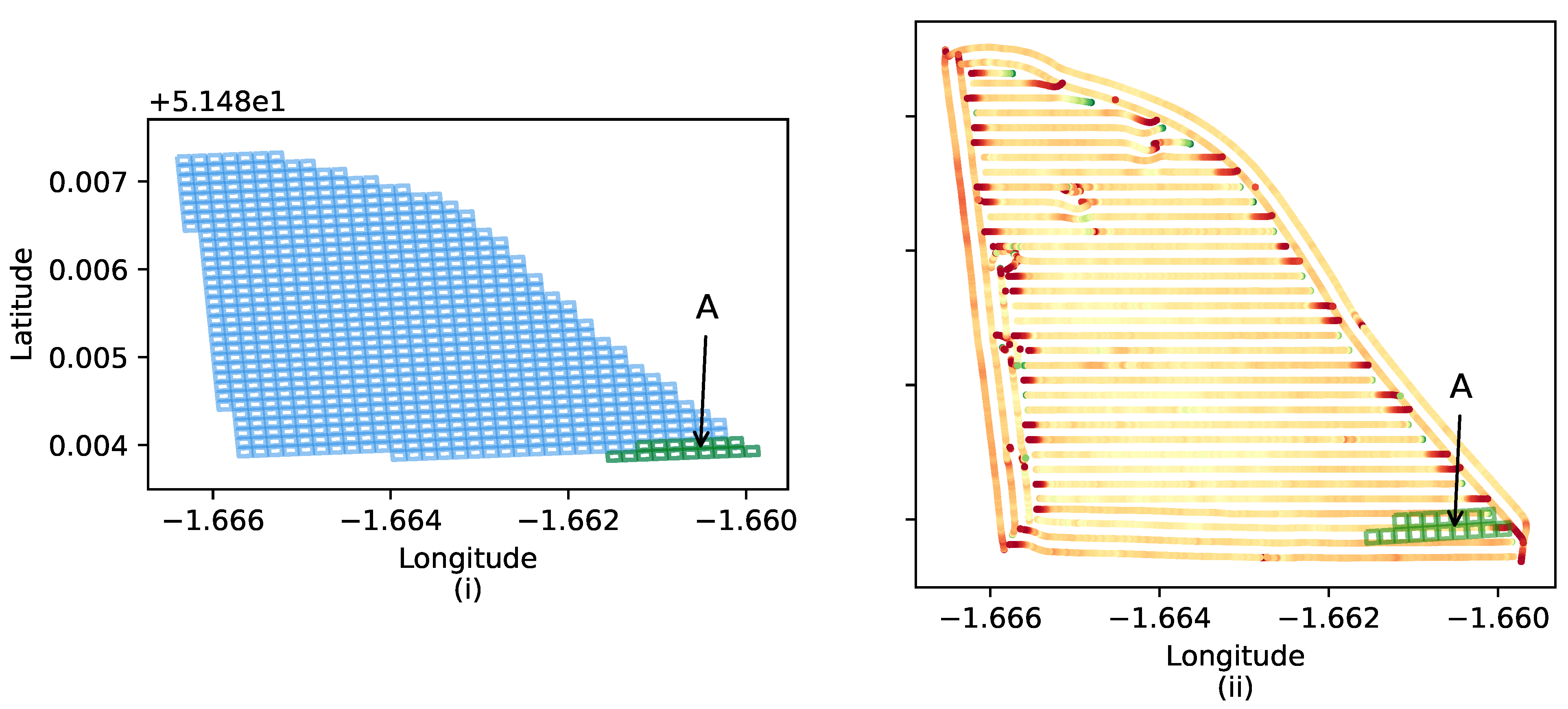
To identify and correct voids, the proposed approach performs the following steps. (1) The boundary map is used to generate a fixed-size grid structure encompassing the entire area of the boundary map. This is illustrated in
Figure 5i and
Figure 6i. (2) For each set of grid coordinates, search the yield map data to determine if such coordinates overlap with the yield map data. (3) Determine any grids whose coordinates do not overlap with the corresponding yield map to constitute a void. The concept is that if a yield map is complete, each small grid in the field boundary map should be contained in the yield map. Otherwise, the grids within the field boundary map, but not within the yield map, constitute part of the void. (4) Finally, a new boundary map is constructed that includes the void.
An example of the process is shown in
Figure 5 and
Figure 6. When a yield map has no void, the coordinates of each grid in the boundary map have a one-to-one mapping to the yield map. For example, for each grid highlighted in green in the boundary map (artefact A in
Figure 5i), there is a corresponding one in the yield map (artefact A in
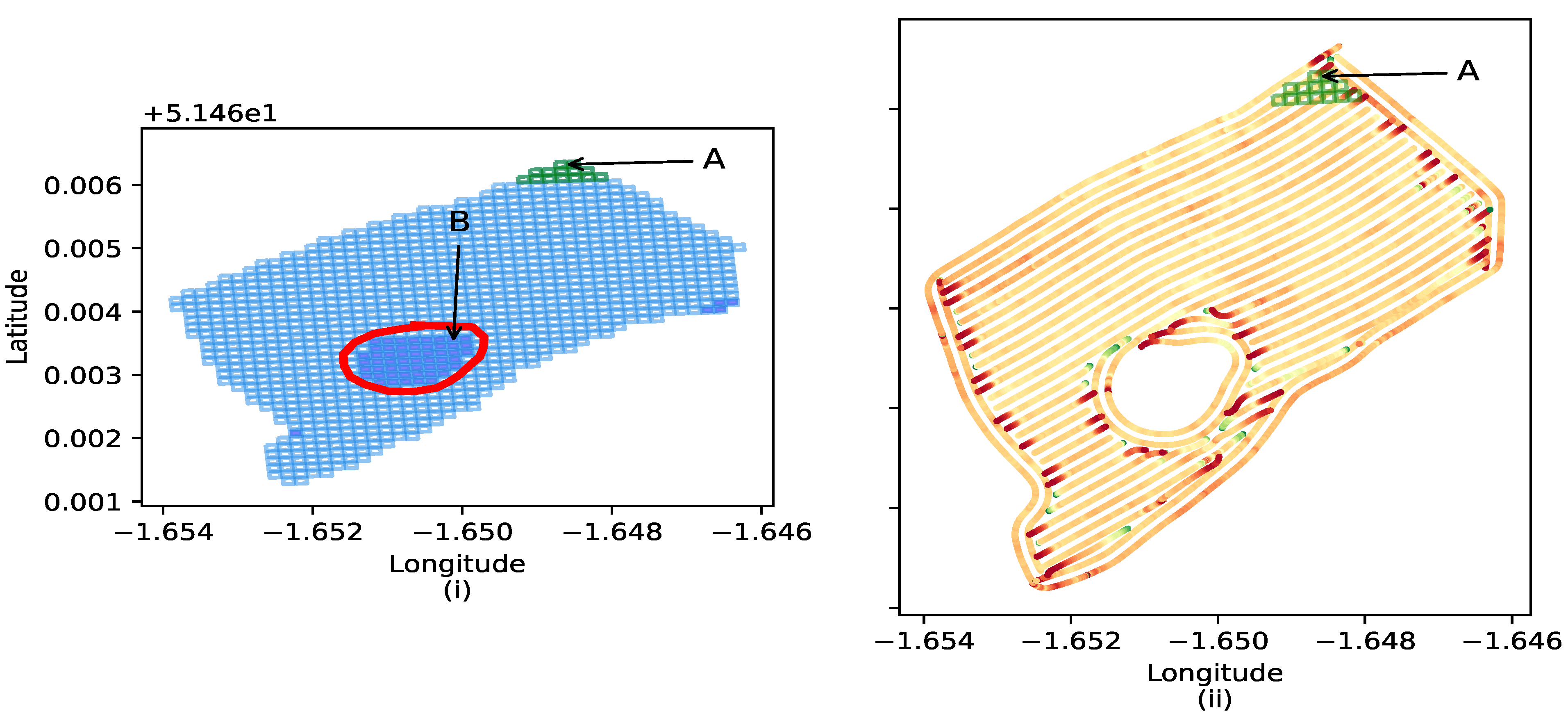
Figure 5ii). For yield maps with a void, however, grids exist in the boundary map without mapping to the yield map. For example, in
Figure 6, the green highlights (artefact A in
Figure 6i) have corresponding ones to the yield map (artefact A in
Figure 6ii). Grids in (artefact B in
Figure 6i), however, have no mapping to the yield map because the void has no corresponding GPS data.
The initial size of the each grid was set to 10 m. This was chosen as the lower limit because the harvest line in the field have the same size. Lowering this value could increase false positives. Different size were tested to determine the optimal grid size that maximises true positive rate. The proposed method is highly computationally efficient and ideal for real-time applications. Unlike computer vision-based techniques that require converting spatial data to images (pixels), which can lead to loss of information, the proposed approach works directly with GPS coordinates, ensuring no information is lost.
4.2. Data Quality Scoring
The data quality scoring technique used in this paper is based on previous research [
13] that uses trust and DQDs to evaluate the quality of heterogeneous IoT data streams in real-time. Trust is a well-established metric that has been used to validate the reliability of unknown sources [
22]. To this end, therefore, given a yield map dataset, the quality score will be given by
The weights
and
are determined by each use case. The goal is for each use case to be able to customise its own quality score. The metric
e is the experience metric. It ensures that a past quality score and current quality score of the same dataset contribute to the overall score of the dataset. Detailed description and implementation of these can be found in our previous research [
11,
13,
22].
4.3. Evaluation Strategy Using Spatial Interpolation
Using yield maps for decision-making requires high-resolution maps [
23]. To this end, several spatial interpolation techniques exist, for example, linear interpolation, inverse distance weighting (IDW), and Kriging [
24]. These work by taking known values (yield) and predicting unknown values in the neighbourhood. This process results in improved maps with clear boundaries showing the variation in yield output of the different field sections.
To evaluate the effectiveness of using DQDs for real-time quality assessment of yield maps, this paper uses IDW as an application example. Any interpolation technique, however, can be used without any changes to the downstream processes.
Inverse Distance Weighting (IDW)
IDW interpolation is a deterministic spatial interpolation method that uses known values with corresponding weights to estimate an unknown value at a particular location [
25]. One IDW method, sometimes referred to as Shepard’s method [
26], is given by the following equation
where z is the estimate at point x, n is the number of surrounding points, and w is given by:
where
and
correspond to the Euclidean distance. Typically values
are
usually used; however, in this paper, grid search was used to obtain the optimal values.
To evaluate the performance of IDW, the root mean squared error (RMSE) was used. This is given by the following equation:
where n is the number of data points and
,
are actual and predicated values, respectively.
5. Evaluation
The system implementation is divided into two stages. In the first stage, spatial errors are classified, and in the second stage, the impact of data quality issues (DQDs) on spatial interpolation is assessed. To evaluate the system’s performance, two experiments were conducted.
The first experiment aims to evaluate the benefits of adding void detection to the spatial error processing data pipeline using a grid approach. The effectiveness of the proposed algorithm is evaluated using a dataset containing fields with and without voids. The algorithm creates a grid of cells from the field boundary map and compares each cell to the yield map. As the grid size affects the algorithm’s performance, a range of grid sizes are compared using accuracy, sensitivity, and specificity as performance metrics.
The second experiment aims to evaluate the efficacy of using a quality score calculated using DQDs that are mapped from spatial errors as a means to assess the quality of yield map datasets. The dataset described in the next section was used. The advantage of using the proposed quality score is that it is not based on a gold standard (weighbridge data). The RMSE of the yield dataset and quality score are calculated before and after filtering spatial errors. The mean of scores of RMSE and quality score for each year are compared.
5.1. Dataset Description
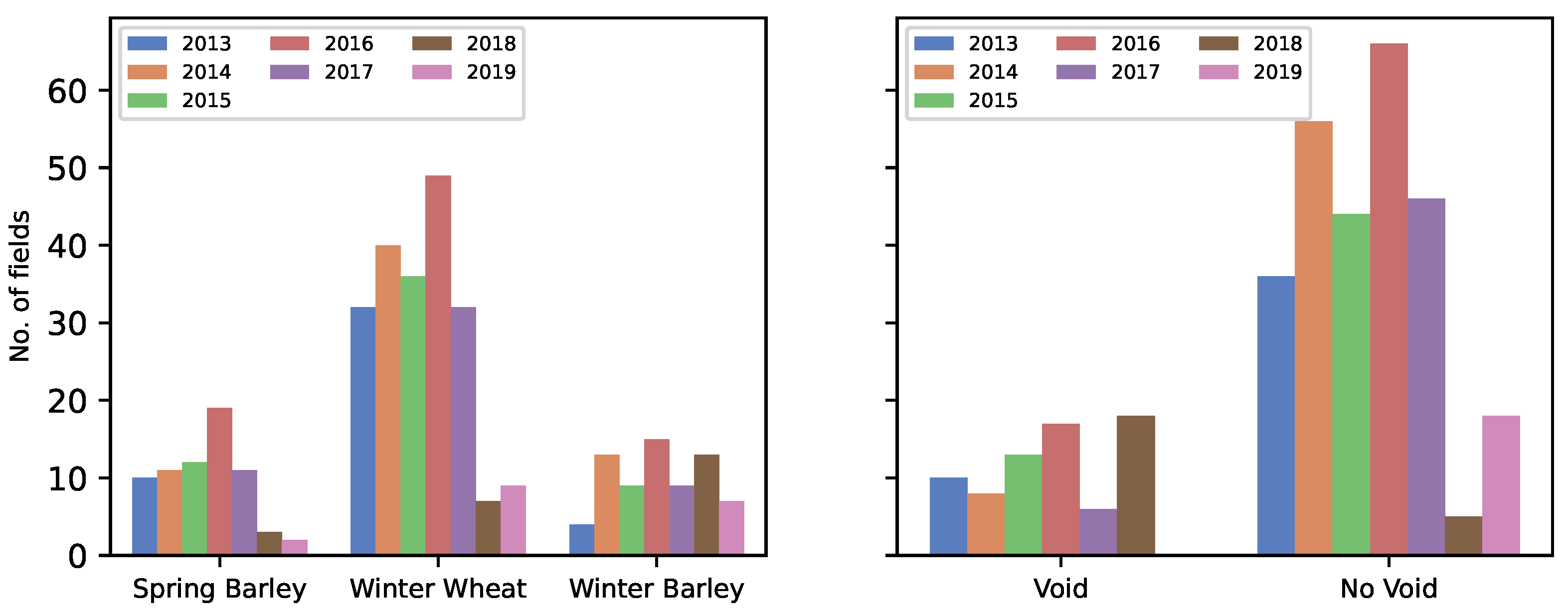
The dataset consists of 524 yield maps collected from 267 fields across 20 farms in the United Kingdom. The biggest field spans over 56.0 hectares; the smallest is approximately 0.1 hectares. The data was collected from 2013 to 2019 and consists of three crops: winter barley, spring barley, and winter wheat. The dataset also includes weighbridge data corresponding to each field. This is used as the true measure of yield per year. A total of 21% of all the yield maps used had voids, and of these, 50% had a high (greater than two tones/per hectare) discrepancy between the measured yield output from the combine and the actual output from the weighbridge.
Figure 7 summarises the dataset with the distribution of crops across fields for each year and the void distribution across fields.
5.2. Results and Discussion
This section is structured into three main parts. The first two sections detail results related to a novel void detection and correction algorithm. Furthermore, they examine the influence of these enhancements on downstream processes, particularly interpolation. The third part evaluates the effectiveness of the data quality dimensions (DQDs) in filtering spatial errors, utilizing spatial interpolation as the evaluation method.
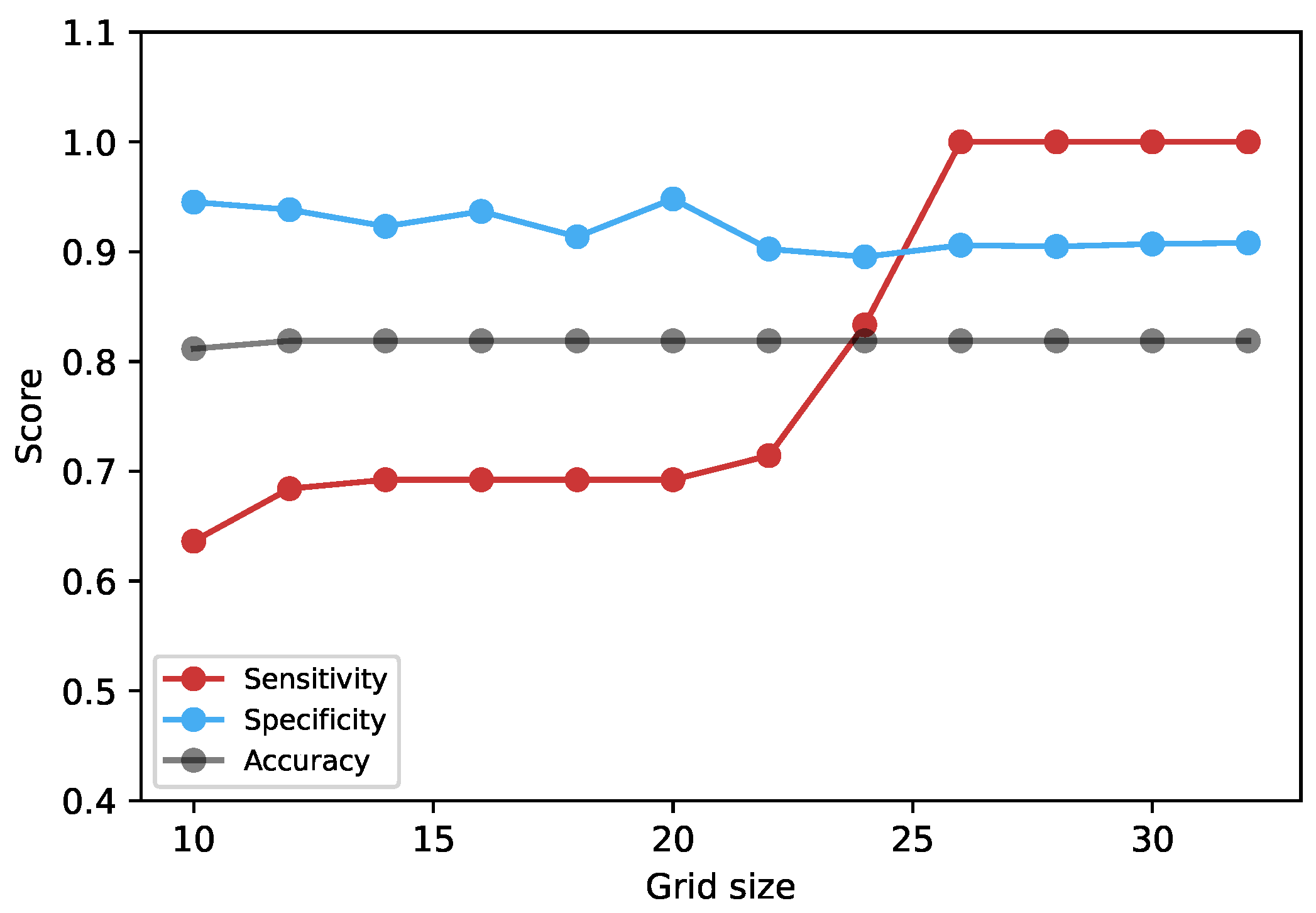
5.2.1. Void Identification
Figure 8 shows the results of the classification algorithm. This is a binary classification problem with yield maps with voids given as positive examples and those without voids considered as negative examples. Yield maps usually contain other kinds of gaps, for example harvest lines (gap between two harvest line) and other anomalies which are not voids, and should not be misclassified as such. Choosing an optimal grid size is important to avoid false positives. Typically the gap between two harvest lines is usually about 10 m. For this reason grid size values below 10 m were not used to avoid this miss identification. Grid sizes above 25 m had the highest score of 100%, 91%, and 82% for sensitivity, specificity, and accuracy, respectively. The main objective of the experiment was to minimise false positives, as this would affect downstream processes. These are defined as below:
where
TP is true positive,
FP is false positive,
TN is true negative, and
FN is false negative.
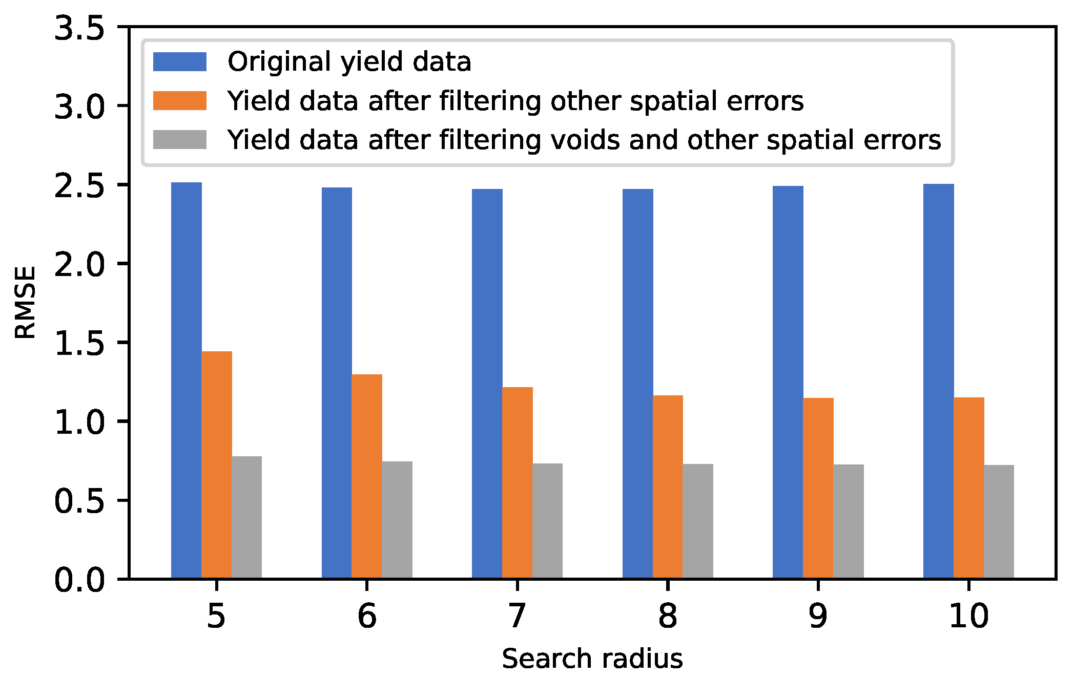
5.2.2. Effects of Void Correction and Other Spatial Errors on RMSE
Figure 9 shows the effects of the presence of voids and other spatial errors on the interpolation process. To assess this effect, the RMSE score after interpolation is used. The RMSE was computed by comparing the interpolated values with the actual yield values from the weighbridge. The lower the RMSE value, the better the interpolation performance, and vice versa. The study compared different search radii values, which also affect interpolation performance. Obtaining an optimal value is critical. Values ranging from 5 to 10 m were used, although there was no significant difference. As shown in
Figure 9, after filtering spatial errors, there was a very significant improvement in the overall RMSE score.
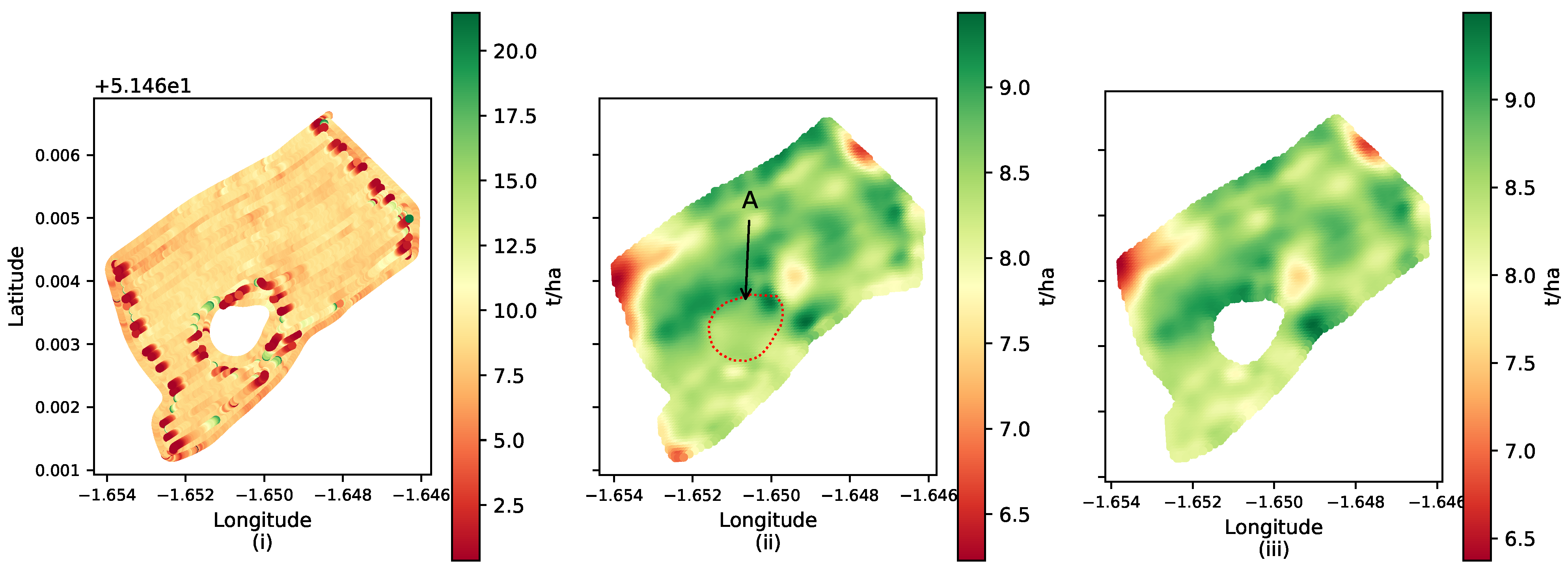
Figure 10i displays the original yield map before interpolation.
Figure 10ii,iii explores the effects of not considering and considering spatial errors on the interpolation process, respectively.
Figure 10ii (artefact A) demonstrates that conventional approaches that do not account for voids and other spatial errors can result in inaccuracies. This can compromise downstream processes such as yield prediction that rely on this data. Additionally, the interpolation process can also impact regions outside of the void, leading to incorrect yield representations and potentially erroneous decision-making, such as in the case of automated fertilizer applications. On the other hand,
Figure 10iii takes into account the presence of voids and other spatial errors, and, therefore, effectively addresses these shortcomings.
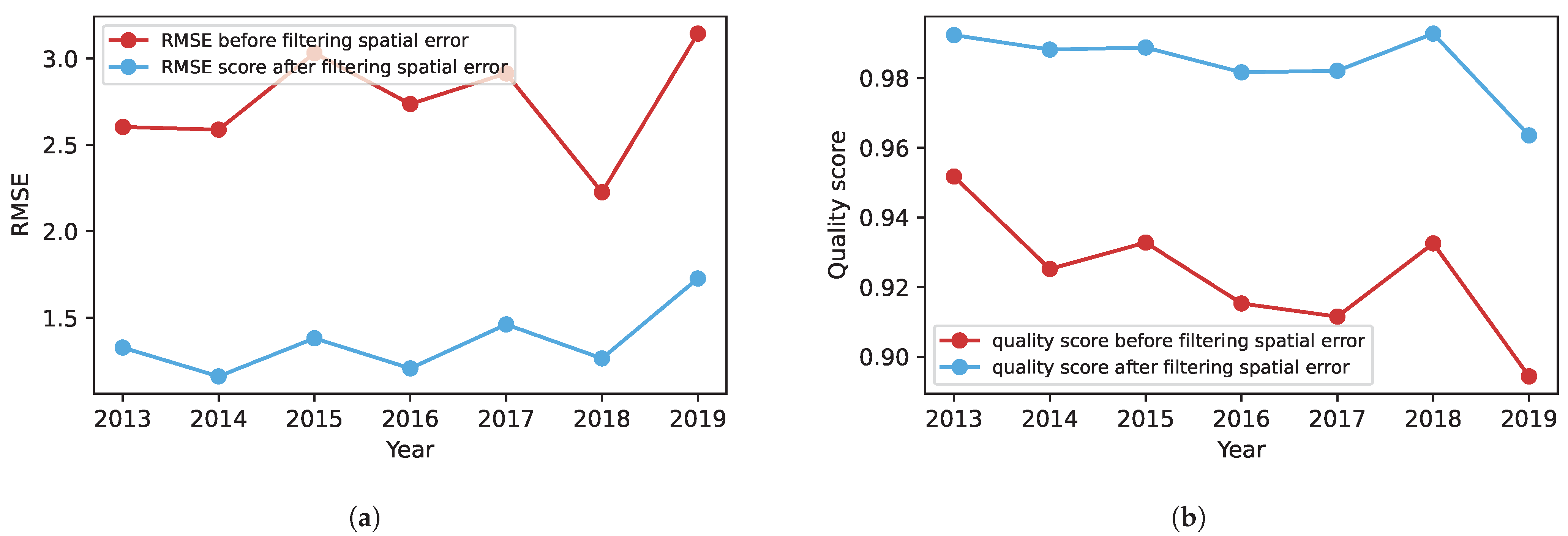
5.2.3. Using DQDs as a Score for Yield Data Quality
Figure 11a,b illustrates the yield data’s average RMSE and quality score for different years, both before and after filtering out spatial errors. Pearson’s correlation coefficient was used to analyse the relationship between the RMSE and the quality score. The comparison was made between the RMSE values before and after filtering and their respective quality scores. An inverse relationship was observed between the RMSE and the proposed quality score. This behaviour is expected since, as the yield data quality improves, the RMSE is anticipated to decrease while the quality score would increase, and vice versa.
The correlation coefficient before filtering out spatial errors was lower than the correlation coefficient after the filtering process. This discrepancy can be attributed to outliers, affecting most interpolation methods and consequently impacting the resulting RMSE score. The stronger correlation observed after filtering out spatial errors suggests that the proposed quality score can be employed as an effective means of assessing yield data quality without requiring a gold standard. The correlation results are summarized in
Table 1 and
Table 2. These are based on the RMSE score presented in
Figure 11.
6. Conclusions
Technological advancements in agriculture have revolutionized farming practices by implementing precision agriculture. This approach leverages data from various processes to make informed decisions and optimize agricultural practices. However, it is essential to acknowledge that data collected from combines can often contain errors resulting from systematic and operator actions, significantly impacting the decision-making process. To address this challenge, several approaches, such as filtering and interpolation methods, have been proposed to mitigate these errors. Nevertheless, finding a comprehensive solution to identify and filter voids or holes in yield maps remains a persistent challenge.
This paper introduces a novel algorithm specifically designed to identify voids in yield maps. The algorithm effectively maps three types of spatial errors, namely GPS errors, yield surges, and voids, to two commonly used data quality dimensions (DQDs): accuracy and completeness. To the best of our knowledge, no existing solution currently employs this approach. The effectiveness of DQDs in filtering spatial errors was evaluated using spatial interpolation techniques. This work has the potential to significantly enhance the performance of downstream processes for yield map data and establish a unified data quality assessment framework based on consistent metrics across multiple data sources.
While this study focused on addressing three specific spatial errors, namely GPS errors, yield surges, and voids, and two common DQDs of accuracy and completeness, our future work will involve the integration of additional spatial errors and DQDs. We will explore the overall impact on the root mean square error (RMSE). Additionally, future research efforts will aim to incorporate larger zones within farms, different crops, and various harvest combines, as these factors can influence the quality of yield maps. Furthermore, most yield maps contain a single void, but there are instances where this number can increase to two or even three and, as the number of voids increases, the algorithm’s accuracy is impacted. Future work will also aim to address this challenge.


 ,
, 


