


Accurate Measurement of Frozen Soil Depth Based on I-TDR

Abstract
:1. Introduction
2. Materials and Methods
2.1. Principles of Soil Impedance Measurement
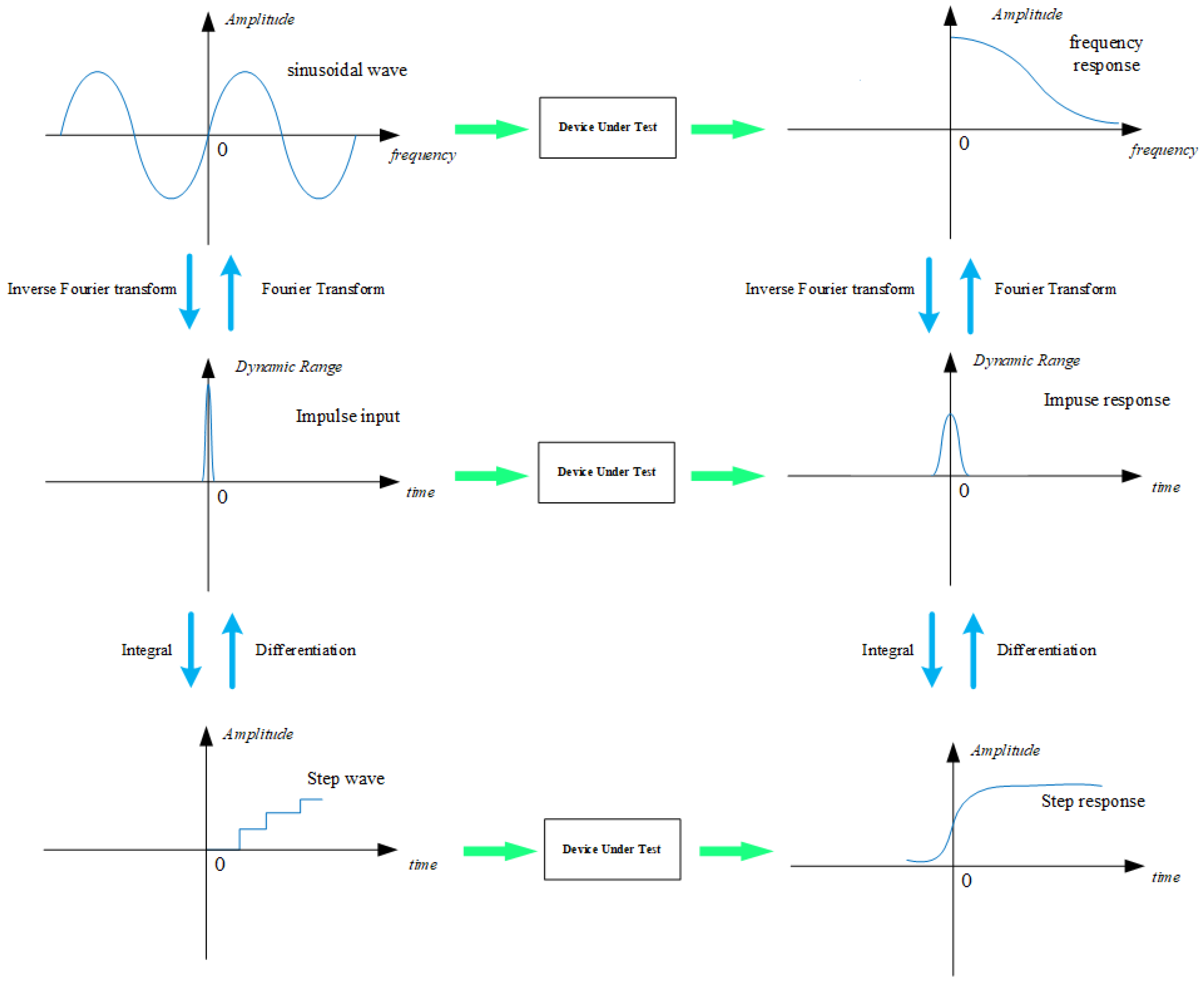
2.2. Principle of Time-Frequency Conversion of Microwave Signal
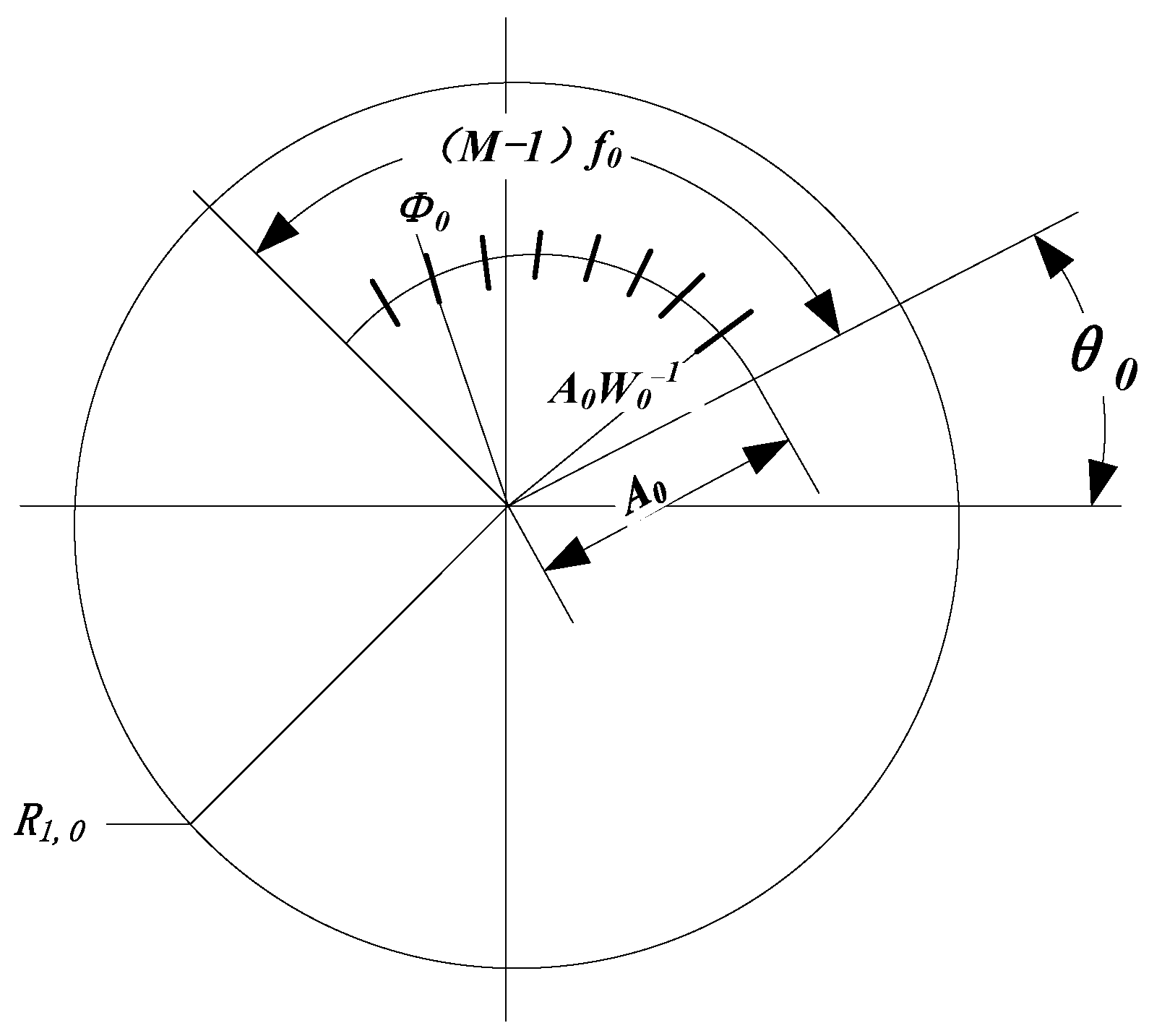
2.3. Wave Crest Recognition Principle Based on Fourier Self-Deconvolution
3. Test Plan for Frozen Soil Frontal Detection Based on TDR
4. Test Plan for Frozen Soil Frontal Detection Based on I-TDR
5. Result and Discussion
6. Conclusions
Author Contributions
Funding
Data Availability Statement
Conflicts of Interest
References
- Zhang, Z.; Ma, W.; Zhang, Z. Scientific Concept and Application of Frozen Soil Engineering System. Cold Reg. Sci. Technol. 2018, 146, 127–132. [Google Scholar] [CrossRef]
- Henry, H.A.L. Climate Change and Soil Freezing Dynamics: Historical Trends and Projected Changes. Clim. Chang. 2008, 87, 421–434. [Google Scholar] [CrossRef]
- Zheng, X.Q.; Van Liew, M.W.; Flerchinger, G.N. Experimental Study of Infiltration into a Bean Stubble Field during Seasonal Freeze-Thaw Period. Soil Sci. 2001, 166, 3–10. [Google Scholar]
- Chen, J.; Xie, X.; Zheng, X.; Xue, J.; Miao, C.; Du, Q.; Xu, Y. Effect of Straw Mulch on Soil Evaporation during Freeze-Thaw Periods. Water 2019, 11, 1689. [Google Scholar] [CrossRef]
- Orakoglu, M.E.; Liu, J.; Tutumluer, E. Frost Depth Prediction for Seasonal Freezing Area in Eastern Turkey. Cold Reg. Sci. Technol. 2016, 124, 118–126. [Google Scholar] [CrossRef]
- Gao, J.; Xie, Z.; Wang, A.; Liu, S.; Zeng, Y.; Liu, B.; Li, R.; Jia, B.; Qin, P.; Xie, J. A New Frozen Soil Parameterization Including Frost and Thaw Fronts in the Community Land Model. J. Adv. Model. Earth Syst. 2019, 11, 659–679. [Google Scholar] [CrossRef]
- Ming, F.; Li, D. A Model of Migration Potential for Moisture Migration during Soil Freezing. Cold Reg. Sci. Technol. 2016, 124, 87–94. [Google Scholar] [CrossRef]
- Zhang, Y.; Horton, R.; White, D.J.; Vennapusa, P.K.R. Seasonal Frost Penetration in Pavements with Multiple Layers. J. Cold Reg. Eng. 2018, 32, 05018002. [Google Scholar] [CrossRef]
- Sharratt, B.S. Freeze-Thaw and Winter Temperature of Agricultural Soils in Interior Alaska. Cold Reg. Sci. Technol. 1993, 22, 105–111. [Google Scholar] [CrossRef]
- Peng, X.; Frauenfeld, O.W.; Cao, B.; Wang, K.; Wang, H.; Su, H.; Huang, Z.; Yue, D.; Zhang, T. Response of Changes in Seasonal Soil Freeze/Thaw State to Climate Change from 1950 to 2010 across China: Soil Seasonal Freeze/Thaw State Changes. J. Geophys. Res. Earth Surf. 2016, 121, 1984–2000. [Google Scholar] [CrossRef]
- Musa, A.; Ya, L.; Anzhi, W.; Cunyang, N. Characteristics of Soil Freeze–Thaw Cycles and Their Effects on Water Enrichment in the Rhizosphere. Geoderma 2016, 264, 132–139. [Google Scholar] [CrossRef]
- Xiao, Z.; Lai, Y.; Zhang, M. Study on the Freezing Temperature of Saline Soil. Acta Geotech. 2018, 13, 195–205. [Google Scholar] [CrossRef]
- Wang, D.; Wang, Y.; Ma, W.; Lei, L.; Wen, Z. Study on the Freezing-Induced Soil Moisture Redistribution under the Applied High Pressure. Cold Reg. Sci. Technol. 2018, 145, 135–141. [Google Scholar] [CrossRef]
- Wang, C.; Lai, Y.; Zhang, M. Estimating Soil Freezing Characteristic Curve Based on Pore-Size Distribution. Appl. Therm. Eng. 2017, 124, 1049–1060. [Google Scholar] [CrossRef]
- Flerchinger, G.N.; Saxton, K.E. Simultaneous Heat and Water Model of a Freezing Snow-Residue-Soil System II. Field Verification. Trans. ASAE 1989, 32, 573–576. [Google Scholar] [CrossRef]
- Flerchinger, G.N.; Saxton, K.E. Simultaneous Heat and Water Model of a Freezing Snow-Residue-Soil System I. Theory and Development. Trans. ASAE 1989, 32, 565–571. [Google Scholar] [CrossRef]
- Bao, H.; Koike, T.; Yang, K.; Wang, L.; Shrestha, M.; Lawford, P. Development of an Enthalpy-Based Frozen Soil Model and Its Validation in a Cold Region in China: An Enthalpy-Based Frozen Soil Model. J. Geophys. Res. Atmos. 2016, 121, 5259–5280. [Google Scholar] [CrossRef]
- Iwata, Y.; Hirota, T.; Suzuki, T.; Kuwao, K. Comparison of Soil Frost and Thaw Depths Measured Using Frost Tubes and Other Methods. Cold Reg. Sci. Technol. 2012, 71, 111–117. [Google Scholar] [CrossRef]
- Aleksic, S.O.; Mitrovic, N.S.; Lukovic, M.D.; Veljovic-Jovanovic, S.D.; Lukovic, S.G.; Nikolic, M.V.; Aleksic, O.S. A Ground Temperature Profile Sensor Based on NTC Thick Film Segmented Thermistors: Main Properties and Applications. IEEE Sens. J. 2018, 18, 4414–4421. [Google Scholar] [CrossRef]
- Wu, B.; Zhu, H.-H.; Cao, D.; Xu, L.; Shi, B. Feasibility Study on Ice Content Measurement of Frozen Soil Using Actively Heated FBG Sensors. Cold Reg. Sci. Technol. 2021, 189, 103332. [Google Scholar] [CrossRef]
- Zhan, W.; Zhou, J.; Ju, W.; Li, M.; Sandholt, I.; Voogt, J.; Yu, C. Remotely Sensed Soil Temperatures beneath Snow-Free Skin-Surface Using Thermal Observations from Tandem Polar-Orbiting Satellites: An Analytical Three-Time-Scale Model. Remote Sens. Environ. 2014, 143, 1–14. [Google Scholar] [CrossRef]
- Leger, E.; Dafflon, B.; Soom, F.; Peterson, J.; Ulrich, C.; Hubbard, S. Quantification of Arctic Soil and Permafrost Properties Using Ground-Penetrating Radar and Electrical Resistivity Tomography Datasets. IEEE J. Sel. Top. Appl. Earth Obs. Remote Sens. 2017, 10, 4348–4359. [Google Scholar] [CrossRef]
- Sudisman, R.A.; Osada, M.; Yamabe, T. Heat Transfer Visualization of the Application of a Cooling Pipe in Sand with Flowing Pore Water. J. Cold Reg. Eng. 2017, 31, 04016007. [Google Scholar] [CrossRef]
- Sveen, S.-E.; Nguyen, H.T.; Sørensen, B.R. Soil Moisture Variations in Frozen Ground Subjected to Hydronic Heating. J. Cold Reg. Eng. 2020, 34, 04020025. [Google Scholar] [CrossRef]
- Qin, Y.; Wang, Q.; Xu, D.; Yan, J.; Zhang, S. A Fiber Bragg Grating Based Earth and Water Pressures Transducer with Three-Dimensional Fused Deposition Modeling for Soil Mass. J. Rock Mech. Geotech. Eng. 2022, 14, 663–669. [Google Scholar] [CrossRef]
- Liu, Z.; Gu, X.; Wu, C.; Ren, H.; Zhou, Z.; Tang, S. Studies on the Validity of Strain Sensors for Pavement Monitoring: A Case Study for a Fiber Bragg Grating Sensor and Resistive Sensor. Constr. Build. Mater. 2022, 321, 126085. [Google Scholar] [CrossRef]
- Cao, D.; Zhu, H.; Wu, B.; Wang, J.; Shukla, S. Investigating Temperature and Moisture Profiles of Seasonally Frozen Soil under Different Land Covers Using Actively Heated Fiber Bragg Grating Sensors. Eng. Geol. 2021, 290, 106197. [Google Scholar] [CrossRef]
- Colliander, A.; Reichle, R.; Crow, W.; Cosh, M.; Chen, F.; Chan, S.; Das, N.N.; Bindlish, R.; Chaubell, J.; Kim, S.; et al. Validation of Soil Moisture Data Products From the NASA SMAP Mission. IEEE J. Sel. Top. Appl. Earth Obs. Remote Sens. 2022, 15, 364–392. [Google Scholar] [CrossRef]
- Wu, S.; Zhao, T.; Pan, J.; Xue, H.; Zhao, L.; Shi, J. Improvement in Modeling Soil Dielectric Properties during Freeze-Thaw Transitions. IEEE Geosci. Remote Sens. Lett. 2022, 19, 2001005. [Google Scholar] [CrossRef]
- Zhang, T.; Jiang, L.; Zhao, S.; Chai, L.; Li, Y.; Pan, Y. Development of a Parameterized Model to Estimate Microwave Radiation Response Depth of Frozen Soil. Remote Sens. 2019, 11, 2028. [Google Scholar] [CrossRef]
- Liu, Z.; Gu, X.; Wu, W.; Zou, X.; Dong, Q.; Wang, L. GPR-Based Detection of Internal Cracks in Asphalt Pavement: A Combination Method of DeepAugment Data and Object Detection. Measurement 2022, 197, 111281. [Google Scholar] [CrossRef]
- Zhang, L.; Zhao, T.; Jiang, L.; Zhao, S. Estimate of Phase Transition Water Content in Freeze-Thaw Process Using Microwave Radiometer. IEEE Trans. Geosci. Remote Sens. 2010, 48, 4248–4255. [Google Scholar] [CrossRef]
- Jadoon, K.; Weihermüller, L.; McCabe, M.; Moghadas, D.; Vereecken, H.; Lambot, S. Temporal Monitoring of the Soil Freeze-Thaw Cycles over a Snow-Covered Surface by Using Air-Launched Ground-Penetrating Radar. Remote Sens. 2015, 7, 12041–12056. [Google Scholar] [CrossRef]
- Vetterli, M.; Kovačević, J.; Goyal, V.K. Foundations of Signal Processing; Cambridge University Press: Cambridge, UK, 2014; ISBN 978-1-107-03860-8. [Google Scholar]
- Lin, C.P. Analysis of Nonuniform and Dispersive Time Domain Reflectometry Measurement Systems with Application to the Dielectric Spectroscopy of Soils: Analysis of TDR Measurements. Water Resour. Res. 2003, 39, 1–11. [Google Scholar] [CrossRef]
- Zhu, Y.; Gao, T.; Fan, X.; Han, F.; Wang, C. Electrochemical Techniques for Intercalation Electrode Materials in Rechargeable Batteries. Acc. Chem. Res. 2017, 50, 1022–1031. [Google Scholar] [CrossRef]
- Voyagaki, E.; Mylonakis, G.; Psycharis, I.N. Sliding Blocks under Near-Fault Pulses: Closed-Form Solutions. In Geotechnical Earthquake Engineering and Soil Dynamics IV; American Society of Civil Engineers: Sacramento, CA, USA, 2008; pp. 1–10. [Google Scholar]
- Heim Weber, G.; de Moura, H.L.; Pipa, D.R.; Martelli, C.; da Silva, J.C.C.; da Silva, M.J. Cable Fault Characterization by Time-Domain Analysis From S-Parameter Measurement and Sparse Inverse Chirp-Z Transform. IEEE Sens. J. 2021, 21, 1009–1016. [Google Scholar] [CrossRef]
- Tan, S.; Hirose, A. Low-Calculation-Cost Fading Channel Prediction Using Chirp Z-Transform. Electron. Lett. 2009, 45, 418. [Google Scholar] [CrossRef]
- Bellanger, M. Digital processing of signals: Theory and practice. In Digital Processing of Signals: Theory and Practice; John Wiley & Sons: New York, NY, USA, 2000; ISBN 978-0-471-97673-8. [Google Scholar]
- Chang, L.; Cui, G. Moiré Fringe Phase Difference Measurement Based on Spectrum Zoom Technology. Telkomnika Indones. J. Electr. Eng. 2013, 11, 6025–6033. [Google Scholar] [CrossRef]
- Lewitt, R.M. Multidimensional Digital Image Representations Using Generalized Kaiser–Bessel Window Functions. J. Opt. Soc. Am. A 1990, 7, 1834. [Google Scholar] [CrossRef]
- Qian, F.; Wu, Y.; Hao, P. An Automated Algorithm of Peak Recognition Based on Continuous Wavelet Transformation and Local Signal-to-Noise Ratio. Appl. Spectrosc. 2017, 71, 1947–1953. [Google Scholar] [CrossRef]
- Lorenz-Fonfria, V.A.; Padros, E. The Role and Selection of the Filter Function in Fourier Self-Deconvolution Revisited. Appl. Spectrosc. 2009, 63, 791–799. [Google Scholar] [CrossRef] [PubMed]
- GB/T 50123–2019; Standard for Geotechnical Testing Method. National Standards of P.R.C.: Beijing, China, 2019.
- Zhao, W.; Qin, H.-B.; Qiang, L. A Calibration Procedure for Two-Port VNA with Three Measurement Channels Based on t-Matrix. Prog. Electromagn. Res. Lett. 2012, 29, 35–42. [Google Scholar] [CrossRef]
- Weiler, K.W.; Steenhuis, T.S.; Boll, J.; Kung, K.J.S. Comparison of Ground Penetrating Radar and Time-Domain Reflectometry as Soil Water Sensors. Soil Sci. Soc. Am. J. 1998, 62, 1237–1239. [Google Scholar] [CrossRef]
- Leoni, A.; Mondot, M.; Durier, F.; Revellin, R.; Haberschill, P. Frost Formation and Development on Flat Plate: Experimental Investigation and Comparison to Predictive Methods. Exp. Therm. Fluid Sci. 2017, 88, 220–233. [Google Scholar] [CrossRef]


| Soil | Cosmid (%) (<0.002 mm) | Powder (%) (0.002–0.02 mm) | Sand Grain (%) (0.02–2 mm) | Bulk Density (g/cm3) |
|---|---|---|---|---|
| Black soil | 19.44 | 22.32 | 58.24 | 1.31 |
| Experimental Equipment | Model |
|---|---|
| Time Domain Reflectometer | Campbell scientific TDR100, Logan, UT, USA |
| DC power supply | TECPEL UTP-3305, Taipei, China |
| Homemade PCB probe | — |
| Adapter cable | ADL BNC-SMACable, Shenzhen, China |
| Soil | Cosmid (%) (<0.002 mm) | Powder (%) (0.002–0.02 mm) | Sand Grain (%) (0.02–2 mm) | Bulk Density (g/cm3) |
|---|---|---|---|---|
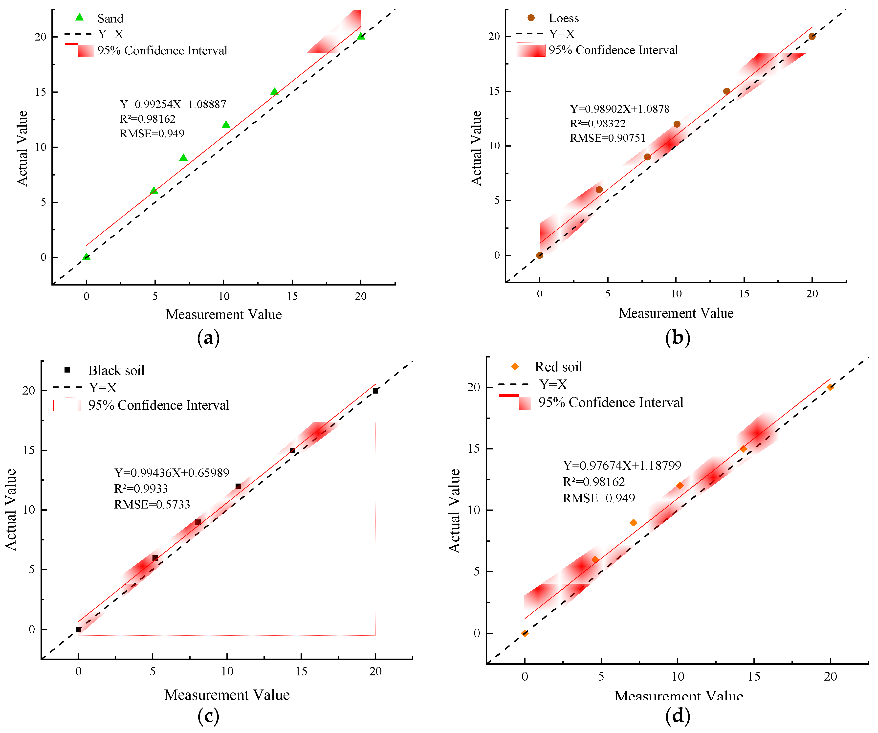
| Sand | 8.08 | 20.36 | 71.56 | 1.54 |
| Loess | 12.46 | 50.32 | 37.22 | 1.70 |
| Red soil | 28.53 | 42.56 | 28.91 | 1.46 |
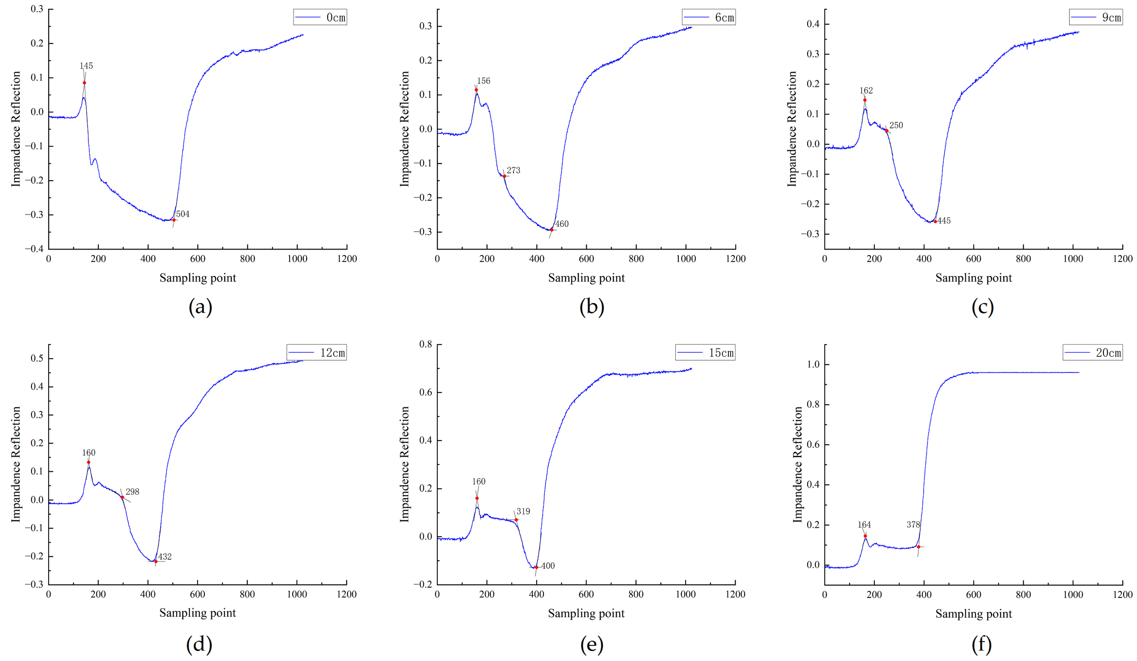
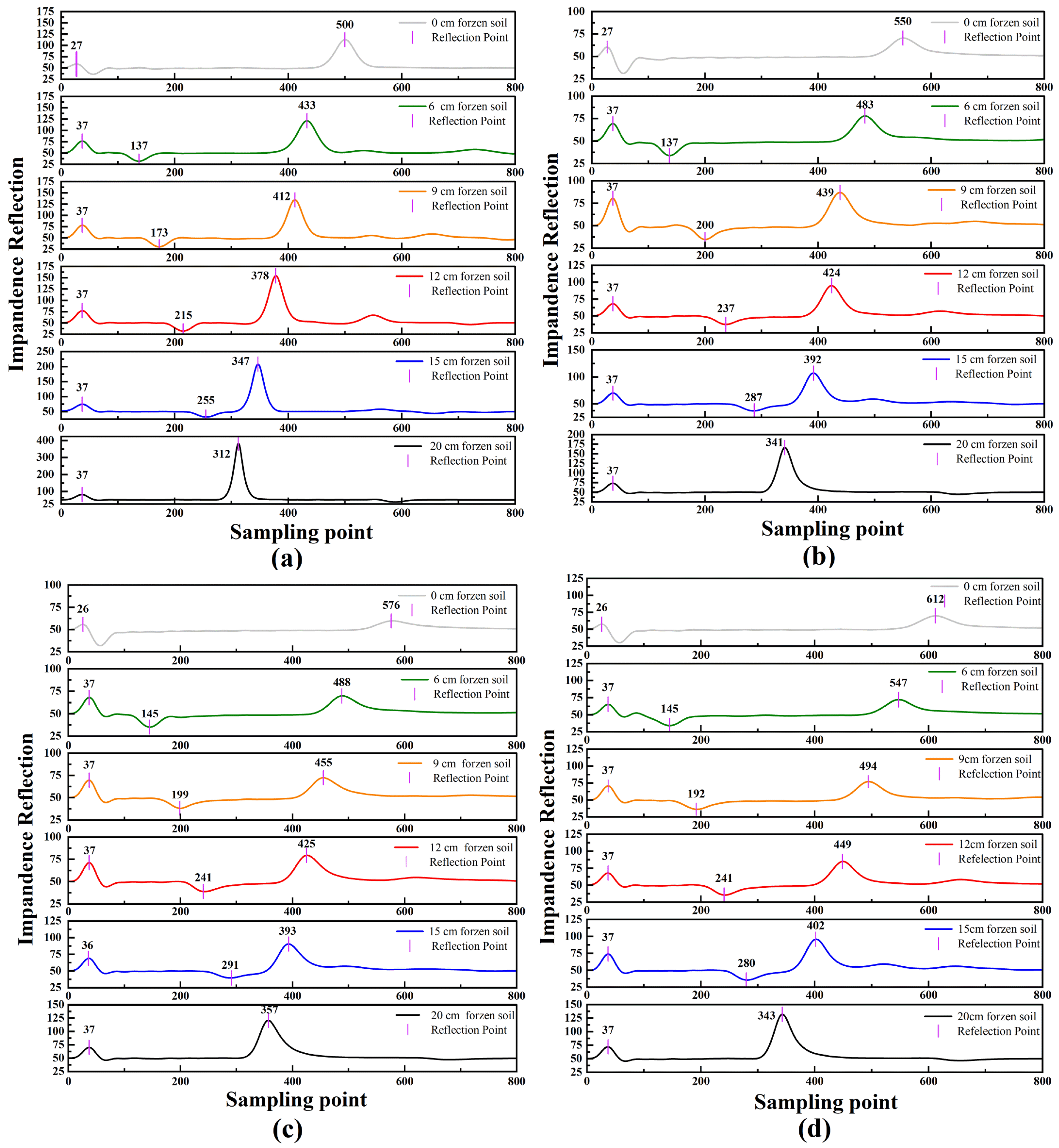
| Depth | Reflection Point Type | 0 cm | 6 cm | 9 cm | 12 cm | 15 cm | 20 cm | |
|---|---|---|---|---|---|---|---|---|
| Soil Type | ||||||||
| Sand | Starting point of reflection | 27 | 37 | 37 | 37 | 37 | 37 | |
| Intermediate reflection point | 137 | 173 | 215 | 255 | ||||
| End reflection point | 500 | 433 | 412 | 378 | 347 | 312 | ||
| Loess | Starting point of reflection | 27 | 37 | 37 | 37 | 37 | 37 | |
| Intermediate reflection point | 137 | 200 | 237 | 287 | ||||
| End reflection point | 550 | 483 | 439 | 424 | 392 | 341 | ||
| Black earth | Starting point of reflection | 26 | 37 | 37 | 37 | 36 | 37 | |
| Intermediate reflection point | 145 | 199 | 241 | 291 | ||||
| End reflection point | 576 | 488 | 455 | 425 | 393 | 357 | ||
| Red soil | Starting point of reflection | 26 | 37 | 37 | 37 | 37 | 37 | |
| Intermediate reflection point | 145 | 192 | 241 | 280 | ||||
| End reflection point | 612 | 547 | 494 | 449 | 402 | 343 | ||
Disclaimer/Publisher’s Note: The statements, opinions and data contained in all publications are solely those of the individual author(s) and contributor(s) and not of MDPI and/or the editor(s). MDPI and/or the editor(s) disclaim responsibility for any injury to people or property resulting from any ideas, methods, instructions or products referred to in the content. |
© 2023 by the authors. Licensee MDPI, Basel, Switzerland. This article is an open access article distributed under the terms and conditions of the Creative Commons Attribution (CC BY) license (https://creativecommons.org/licenses/by/4.0/).
Share and Cite
Qin, H.; Mu, Z.; Jia, X.; Kang, Q.; Li, X.; Xu, J. Accurate Measurement of Frozen Soil Depth Based on I-TDR. Agronomy 2023, 13, 1389. https://doi.org/10.3390/agronomy13051389
Qin H, Mu Z, Jia X, Kang Q, Li X, Xu J. Accurate Measurement of Frozen Soil Depth Based on I-TDR. Agronomy. 2023; 13(5):1389. https://doi.org/10.3390/agronomy13051389
Chicago/Turabian StyleQin, Haoqin, Zhiquan Mu, Xingyue Jia, Qining Kang, Xiaobin Li, and Jinghui Xu. 2023. "Accurate Measurement of Frozen Soil Depth Based on I-TDR" Agronomy 13, no. 5: 1389. https://doi.org/10.3390/agronomy13051389