Article

Spatial Analysis of Soil Moisture and Turfgrass Health to Determine Zones for Spatially Variable Irrigation Management

1
Department of Geography, Brigham Young University, Provo, UT 84602, USA
2
School of Water, Energy and Environment, Cranfield University, Cranfield, Bedfordshire MK43 0AL, UK
3
Department of Plant and Wildlife Sciences, Brigham Young University, Provo, UT 84602, USA
*
Author to whom correspondence should be addressed.
Agronomy 2023, 13(5), 1267; https://doi.org/10.3390/agronomy13051267
Submission received: 15 March 2023 / Revised: 20 April 2023 / Accepted: 25 April 2023 / Published: 28 April 2023
(This article belongs to the Special Issue The Importance of Soil Spatial Variability in Precision Agriculture)

Abstract

:
Irrigated turfgrass is a major crop in urban areas of the drought-stricken Western United States. A considerable proportion of irrigation water is wasted through the use of conventional sprinkler systems. While smart sprinkler systems have made progress in reducing temporal mis-applications, more research is needed to determine the most appropriate variables for accurately and cost-effectively determining spatial zones for irrigation application. This research uses data from ground and drone surveys of two large sports fields. Surveys were conducted pre-, within and towards the end of the irrigation season to determine spatial irrigation zones. Principal components analysis and k-means classification were used to develop zones using several variables individually and combined. The errors associated with uniform irrigation and different configurations of spatial zones are assessed to determine comparative improvements in irrigation efficiency afforded by spatial irrigation zones. A determination is also made as to whether the spatial zones can be temporally static or need to be re-determined periodically. Results suggest that zones based on spatial soil moisture surveys and simple observations of whether the grass felt wet or dry are better than those based on NDVI, other variables and several variables in combination. In addition, due to the temporal variations observed in spatial patterns, ideally zones should be re-evaluated periodically. However, a less labor-intensive solution is to determine temporally static zones based on patterns in soil moisture averaged from several surveys. Of particular importance are the spatial patterns observed prior to the start of the irrigation season as they reflect more temporally stable variation that relates to soil texture and topography rather than irrigation management.

1. Introduction

Urban development in the Southwest region of the USA has expanded significantly in recent years, placing strain on the already limited freshwater supply [1]. This problem has been exacerbated by recent drought, with over 30% of the Western USA experiencing “extreme” or “exceptional” drought during 2022 (https://droughtmonitor.unl.edu/, accessed 20 September 2022). The conversion of land to urban areas throughout the USA has meant that more acres of irrigated turfgrass (>40 million acres) are now grown in the USA than irrigated corn, wheat and fruit trees combined [2]. Although turfgrass irrigation requires substantial amounts of the scarce freshwater supply in the west, it also provides several key ecosystem services in urban areas, such as cooling the air through evapotranspiration, reducing energy consumption for building, cooling, reducing storm-water-related flooding, increasing ground water recharge, reducing soil erosion, fixing carbon in the soil [3], cleaning noxious gases from the air [4], and reducing wildfire hazard [5]. Furthermore, grass can help combat global warming because it is particularly effective at taking carbon from the atmosphere and fixing it in the soil as organic matter [6,7]. In soils where grass is grown, organic carbon levels are often twice as high as those in soils where other types of vegetation are cultivated [8]. Therefore, healthy grass is a key asset in urban environments and could help mitigate global warming effects.
Despite the advantages of turfgrass over other urban surfaces in terms of temperature regulation, it has been estimated that in semi-arid areas, approximately 60% of household water is used to irrigate lawns [9] and this proportion is likely to be higher for institutions that do not have residential functions. Furthermore, up to 50% of turfgrass irrigation water is estimated to be wasted [9] due to temporal and spatial mis-applications. The US EPA has implemented the “WaterSense” program which addresses temporal mis-application issues with irrigation controllers to tailor watering schedules based on local weather conditions. This modification alone can reduce irrigation water use by 15% [9]. Orta et al. [10] reported a 30% reduction in water use through sub-surface drip irrigation of turfgrass compared to sprinkler irrigation. The EPA is considering developing irrigation scheduling that is controlled by soil moisture sensors [9] like those being used with agricultural variable rate irrigation systems such as that of Liakos and Vellidis [11]. In such systems, spatial zones have been determined and there are soil moisture sensors in each zone which determine irrigation scheduling and the amount that should be applied using a variable rate central irrigation pivot. The approach implicitly assumes that there is no appreciable variation in soil moisture within the zones and that the sensors are placed in locations that are representative of the soil moisture for the whole zone. Canopy temperatures have been measured by some to assess crop water stress in agricultural fields to determine VRI zones [12]. In contrast to agricultural systems, turfgrass does not produce a crop that can be sold to offset the cost of sensors and technology for precise irrigation. In addition, the ability to irrigate more precisely in the urban turfgrass context has, until recently, been largely lacking due to outdated and inefficient irrigation systems as well as the high cost and complexity of sensor technology.
Affordable technologies have emerged in recent years to address the urban water crisis, including sprinkler heads that utilize “valve-in-sprinkler-head technology” such as those produced by Hunter, Rainbird, and Toro. Unlike the conventional practice of uniformly applying water across a zone with the rate determined by the driest part of the zone, this technology provides individual control of each sprinkler head, so each sprinkler head has its own zone of influence. Many residential customers completely ignore spatial and temporal variability in soil moisture and turn on their sprinkler systems to water every other day for 20 or 30 min in every zone at the beginning of the season, and never adjust those levels until they turn the sprinklers off at the end of the season. Clearly, more informed irrigation scheduling and zoning is needed. New-generation soil moisture tension sensors improve accuracy and the simplicity of use of soil moisture sensors, and turfgrass can be monitored using drones equipped with cameras that record wavelengths of light that are sensitive to plant health. For applications that cover large areas of turfgrass, freely available satellite imagery could be used to inform plant health; however, for applications where the area is smaller such as a single sports field, these satellite images do not give the spatial resolution necessary for effectively applying spatially variable rate irrigation. Finally, smart controllers allow the incorporation of multiple information layers, with weather data, to precisely control irrigation.
The main challenges in determining spatial zones for turfgrass irrigation revolve around what variables should be measured to determine the zones. Being able to observe variables inexpensively and determine the zones in cost-effective ways, especially if they need re-assessing periodically or before each irrigation event, is crucial. Straw and Henry [13] showed for two turfgrass fields, that during a dry-down period, the zones that identified similarities in volumetric water content (VWC), normalized difference vegetation index (NDVI) and penetration resistance changed, so the potential change in zones over time must be investigated. The current research uses data from ground and drone surveys of two large sports fields on the Brigham Young University Campus. One field has sprinklers with traditional zones and the other has valve-in-head sprinkler technology so there is more potential for spatially modifying zones. The surveys were conducted pre-, within and towards the end of the irrigation season. The effectiveness of different variables from the surveys for determining spatial zones to inform soil moisture applications was assessed. Straw et al. [14] compared the data on soil moisture and grass health obtained from mobile and handheld devices for monitoring turfgrass in sports fields. They showed that for NDVI and soil moisture, mobile and handheld devices showed similar spatial patterns but for penetration resistance they did not.
Large institutions are more likely to find developing spatial zones economically feasible in the first instance, as irrigation typically forms a larger proportion of their water bills and they have a greater capacity to invest in expensive mobile equipment and sensors for monitoring patterns of soil moisture and grass health. However, the methods developed here should have the potential to be transferred to the residential turfgrass irrigation sector in the future. This would mean a change in the scale of inquiry and decrease in the budget for sensing, so the cost of the equipment needed to make various measurements on which to base spatial zones is briefly considered here. We also investigate the utility of observations that can be made without equipment but are instead based on human perceptions, such as those investigated by Straw et al. [15].
The current research is unique and distinct from other research that has been published in the MDPI journal Agronomy about turfgrass. There have been several special issues that have looked at simulations for improving turfgrass performance during climate change [16], stress biology [17] and genetics and breeding of different quality traits [18,19]. However, this paper looks at applying principles of precision agriculture to the spatial irrigation management of turfgrass to reduce wasted water. This issue is not addressed by other papers in Agronomy special issues related to Turfgrass.

2. Materials and Methods

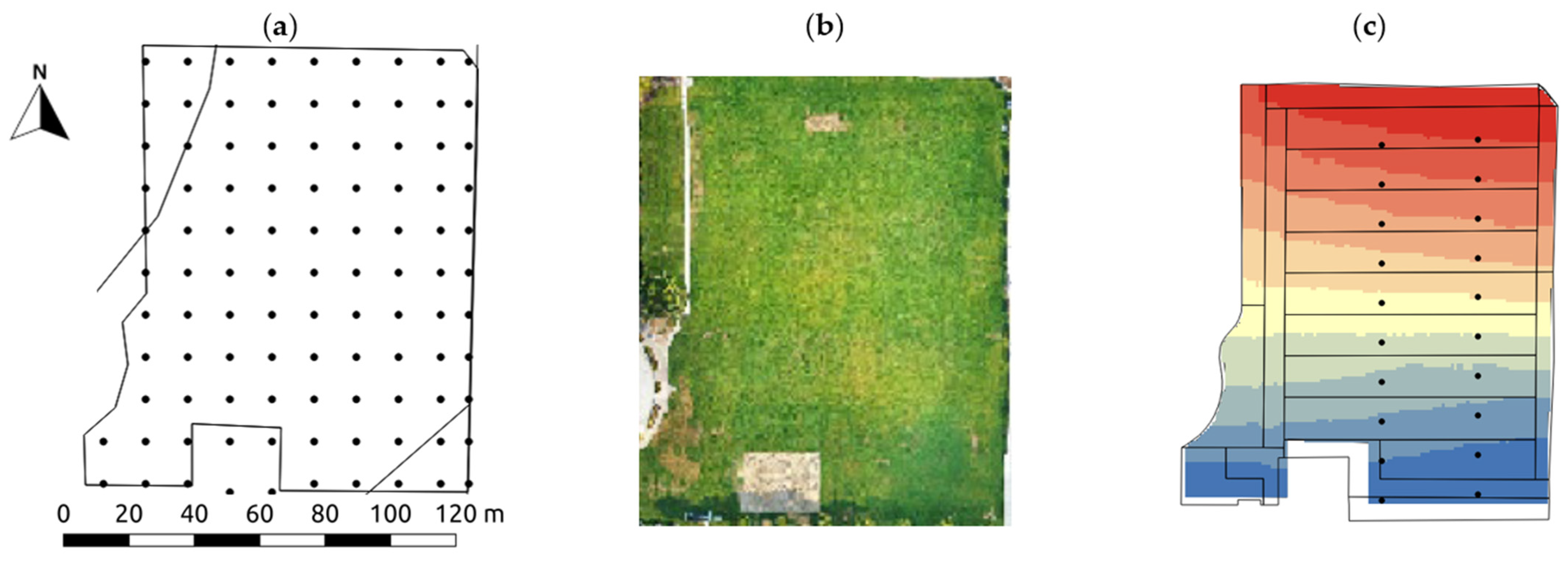
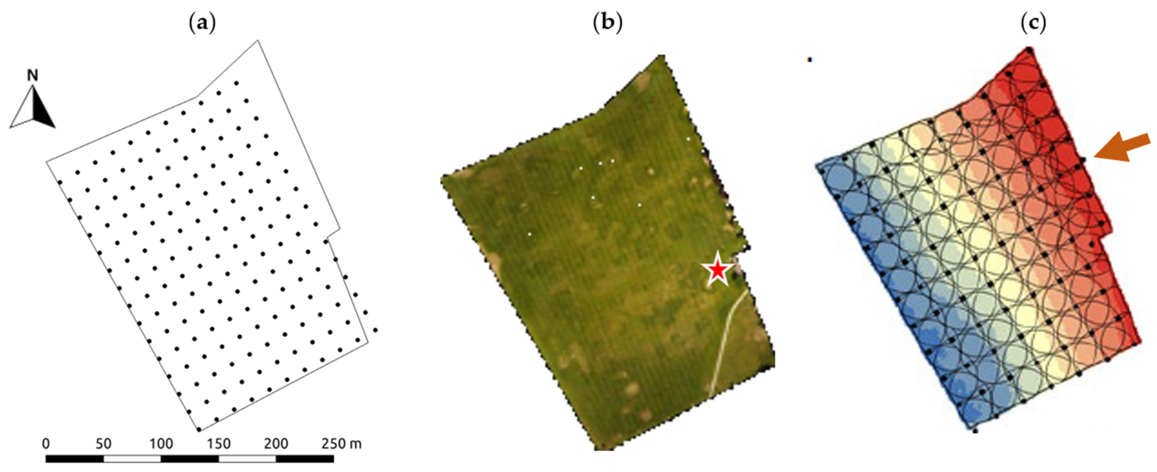
2.1. Field and Drone Surveys

Two general-purpose sports fields that are used for almost daily general student recreational use, rather than competitive sports, on BYU campus were the field sites used for this work. Both fields have Kentucky bluegrass (Poa pratensis L.) turf. Harmon field (40.256 N, 111.644 W) has a gentle N–S running slope and the field dimensions are approximately 150 m (N–S) by 115 m (E–W), Figure 1c. Temple field (40.262 N, 111.644 W) has a slightly steeper NE–SW running slope and the field dimensions are approximately 200 m (NW–SE) by 150 m (NE–SW) Figure 2c. The Harmon field is used for summer sports camps during the irrigation season and this results in quite uniform traffic in all areas of the field; however, in other months student activities tend to be concentrated in the west of the field close to the building and a terrace where outdoor meals are served. In addition, activities tend to occur in the south of the field which is closer to the parking area and halls of residence. For the Temple field, activities and trampling tends to be concentrated in central parts of the field, mostly close to the sports equipment shed indicated by a star in Figure 2b.
Harmon field has traditional sprinkler zones installed which generally run E–W across the field in parallel with the elevation (Figure 1c). However, at the edges of the field, zones run N–S counter to the elevation patterns. In the 2021 irrigation season, field managers applied 30% less water to the 3 zones at the bottom of the slope. The NRCS web soil survey website (https://websoilsurvey.sc.egov.usda.gov/App/WebSoilSurvey.aspx, accessed, 30 May 2021) classified the soil in the Harmon field as 3 types: Taylorsville silty clay loam with 1 to 3 percent slopes, Pleasant Grove gravelly loam with 3 to 6 percent slopes, and Sterling gravelly fine sandy loam with 1 to 3 percent slopes covering 91.5, 5.5 and 3% of the field area, respectively (see Figure 1a). The two less prevalent soil types are found only in the NW and SE corners of the field. A survey of top-soil texture along two N–S running transects towards the center of the field (Figure 1c) completed in September 2021 showed a consistent sandy loam texture rather than silty clay loam. Silt content was, however, shown to be greatest in the center and eastern portions of the field where the Taylorsville silty clay loam was supposed to dominate.
Temple field has new valve-in-head sprinklers where each sprinkler head can form its own zone. Figure 2c shows the area covered by each sprinkler head as a black circle with radius of approximately 27 m. The sprinkler heads are spaced at 20 m so that there is overlap (Figure 2c) between the areas watered by each sprinkler head. The sprinkler heads in temple field were installed in NW–SE running lines that are consistent with changes in elevation running across the slope (Figure 2c). Due to a lack of detailed spatial information to base spatial zones on in this field, in the 2021 irrigation season field managers applied 30% less water to the 3 rows of sprinkler heads at the bottom of the slope. The NRCS web soil survey classified the soil in the Temple field as all of one type, the Pleasant Grove gravelly loam with 3 to 6 percent slopes; however, a survey of top-soil texture along two NW–SE running transects towards the center of the field (see Figure 4c) showed soil textures varying between Clay loam, Loam and Sandy Loam. Some of the patterns of soil texture observed seem to account for non-typical patterns of soil moisture in relation to relative elevation. For example, there were some clayey soils and even gleiing observed at the top of the slope and sandier soils near the bottom of the slope. The gleying also happened to occur where a higher density of sprinkler heads has been installed at the central eastern parts of the field due to the narrowing of the field in this area (see arrow in Figure 2c). Figure 8c shows that some locations in this area of the field are receiving water from as many as 6 or 7 sprinkler heads. Most evident in this field was sudden, unpredictable changes in soil texture. This may have something to do with two pipelines that have been installed under this field in recent years. Construction workers likely re-filled the areas above the pipeline with sand rather than soil. In addition, this field is part of an alluvial fan which could also account for some of the sudden changes in soil texture within the field.
Ground surveys of the fields were performed on a 15 m and 20 m grid for Harmon and Temple fields, respectively (Figure 1a and Figure 2a). This ensured, given the size of the fields, that more than 100 sample locations were available for variogram computation and kriging following the guidelines of Webster and Oliver [20]. However, for Temple field in September 2021, the survey was linked to the collection of soil samples for texture analysis which is expensive, so observations were only made along two transects and at sensor locations (see Black dots in Figure 4c). Straw et al. [13] sampled sports fields comparing several grids with smaller sampling intervals; however, their fields were smaller than those used in this study and would not have had sufficient sampling points (>100) to compute a reliable variogram at a 15 m interval. As irrigation was largely uniform during the study period, the spatial field surveys were scheduled, pre-, mid- and towards the end of the irrigation season. The pre-irrigation season sampling in March/April should capture natural spatial patterns in soil moisture that relate to permanent features of the field such as soil texture and topographic variations. The mid-irrigation season sampling should help identify if any particular areas are being over-watered. Finally, the end of irrigation season sampling in September should accentuate any patterns of grass health caused by drought/over-watering during the season.
Harmon field was sampled pre-irrigation in March 2021, it was sampled twice (survey a and survey b) mid-irrigation-season in August 2021, (August 2021a+b) and was sampled at the end of the irrigation season in September 2020 and September 2021. Temple field was sampled pre-irrigation-season in April 2022, in the middle of the irrigation season in July 2021 and the end of May 2022. Finally, at the end of the irrigation season Temple field was surveyed in September 2021.
Figure 3 shows the monthly average temperatures and precipitation totals for Provo, UT, USA compared to 30 year normals. This will allow evaluation of each survey time as to whether it was wetter or dryer, hotter or cooler than normal. Table 1 summarizes the observations that were made during each survey. Handheld sensors such as a Delta T theta probe, Trimble GreenSeeker NDVI sensor and FieldScout greenindex+ Turf app were used to measure soil volumetric water content (VWC) and normalized difference vegetation index (NDVI), the greenness of grass, or grass health on the 15 m and 20 m grids across both fields. Delta T theta probes currently cost about 1500 USD, Trimble GreenSeeker handheld devices cost about 650 USD, and the FieldScout GreenIndex+ Turf app and board costs 100 USD. There was no equipment cost for estimating % dead or discolored grass and the wet/dry soil indicator. Such observations are similar to the athlete perceptions used to characterize within-field variability by Straw et al. [15] that were shown to correspond with measured properties.
A DJI Phantom 4 drone flown at 119 m above ground level equipped with a 12 mp (4000 × 3000) camera and a Sentera Single Sensor NDVI was used to capture RGB and NDVI imagery with pixel sizes of 2 cm and 6 cm, respectively, and a digital surface model (DSM) of the fields (Table 1). The imagery was stitched together and processed in Drone Deploy (https://www.dronedeploy.com, accessed, 1 December 2022) to create image orthophoto mosaics of each field. Visual Atmospheric Resistance Index (VARI) data, a vegetation index which uses only the RGB wavelengths, was also calculated from the drone imagery. Several derived topographic attributes were calculated in SAGA GIS from the DSM (Table 1). The drone and camera equipment costs about 3000 USD as well as a subscription to the data/image processing website (Drone Deploy). Drone surveys for research purposes also require that the drone operator has a Federal Aviation Administration Part 107 Remote Pilot Certificate. In addition, on a university campus and in some urban areas, health and safety forms must be submitted and approved before each flight and flights are prohibited over some fields that are too close to airports or hospitals that provide air ambulance services.

2.2. Statistical Methods

Ground survey data were kriged to a 1 m grid and drone data were resampled to a 1 m grid to aid in the speed of data processing. Pearson correlations and the bi-variate local Moran’s I (LMI) [23] were used to investigate the consistency of patterns between soil moisture and grass health from different surveys.
In precision agriculture, a common approach to define management zones is to use several inexpensive, densely sampled variables that are related to the variable to be managed and then determine zones from these data using principal components analysis (PCA) and K-means classification [24]. Khosla et al. [25] recommended using multiple variables to define management zones in agricultural crops, rather than relying on a single variable. K-means was used to classify individual variables and composite variables from principal components analysis (PCA) into different numbers of zones. The vegetation indices and topographic attributes derived from drone surveys showed a lot of fine-scale detail that would not be useful in determining management zones so their use was not considered as the sole variable upon which to base a classification. Instead, they were only considered as part of classifications that included all variables for Harmon field in September 2020 and Temple field for the April 2022 survey. The number of zones associated with the greatest break of slope in the associated scree plot (Figure 4b) was used as the optimum number of zones. Zones were then defined using ESRI shapefiles (Figure 4c, black lines).
Using existing zones (Figure 1c and Figure 2c) and the optimal zones determined using individual variables and combinations of variables, average VWC per zone and per field were calculated from the 1 m kriged VWC data. The mean absolute errors, and summary statistics of the errors, associated with irrigating to field and zone average VWC, were calculated with reference to the 1 m kriged VWC data. The errors for zones defined using different variables and for VWC zones from different times were compared.

3. Results and Discussion

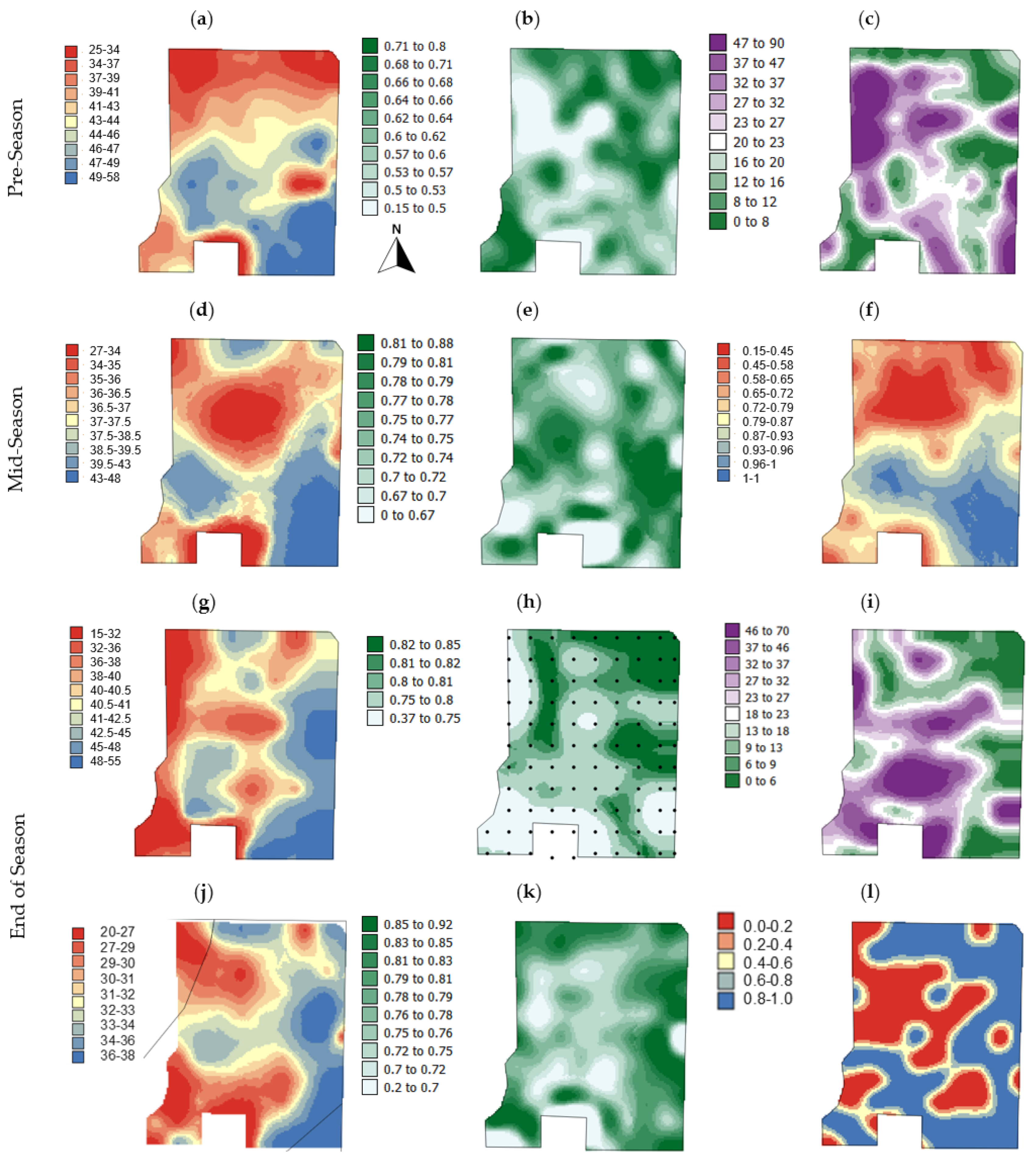
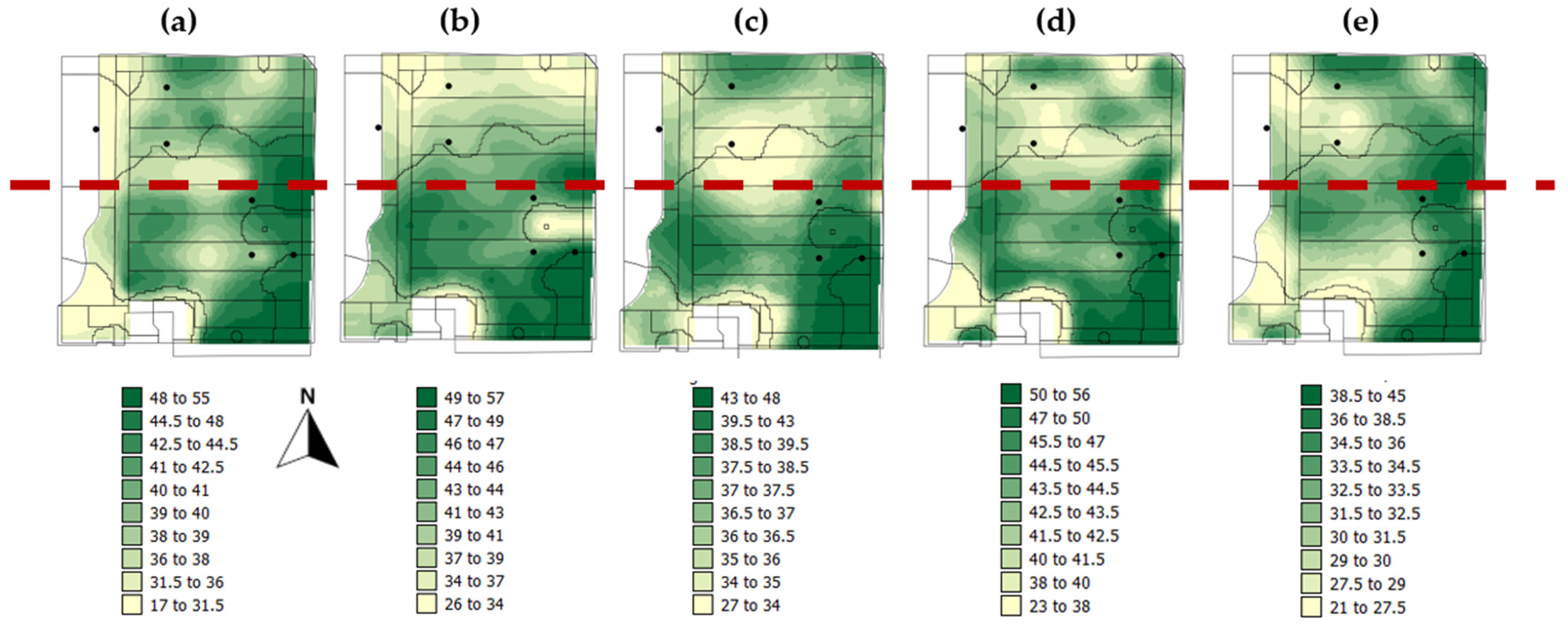
3.1. Harmon Field—Spatial and Temporal Patterns

Harmon field had similarities in the patterns shown in the maps produced from interpolated ground survey variables and these values had moderate correlations with each other (±0.3–0.7, Figure 5). For example, there are similarities in the location of the areas with a high percentage of dead or discolored grass, and VWC. There are also similarities between the patterns in these maps and those shown for NDVI (Figure 5). Previous studies have shown links between lack of soil moisture and grass health or the presence of dead or discolored grass [26,27]. Maps (Figure 5) also showed similarities in the patterns of the variables that do not need expensive equipment to measure them (e.g., % dead grass and wet/dry IND) and patterns of variables that require expensive equipment for measurement. This shows promise for the potential to transfer the approaches developed here to the residential context and also agrees with previous findings of Straw et al. [15] that showed that athlete perceptions of soil status could be relatively accurate for some variables.
Each of the variables shown in Figure 5 seems to show a dominant E–W pattern in the Harmon field with high values of VWC and NDVI and low values for dead grass in the east of the field, and the reverse in the west of the field. These patterns show consistency with the patterns of degree of slope (Figure 6d). There is also a N–S pattern for VWC (March 2021) and the wet/dry indicator (August 2021a). Others have found similar links between small topographic variations and changes in soil moisture and NDVI or other indications of plant health [28,29]. Indeed, such variations account for the importance of derived topographic attributes and vegetation indices in the digital soil mapping approach [30,31,32,33].
The N–S pattern of VWC (Figure 5) is logical given the main direction of the slope of the field and the consistency in soil texture within the field. However, at first glance at the field, one would expect the N–S topographic pattern to be the dominant feature of variation in the field rather than the E–W variation as the downhill slope N–S is far more pronounced than the W–E downhill slope. The E–W variation in grass health, with poorer health in the west, may partially be a function of greater foot traffic in the west of the field close to the pavilion/terrace area of the building. Indeed, symptoms of severe compaction, such as standing water at the surface which percolated away following insertion of a theta probe, were observed in the western parts of the field and previous studies have shown the detrimental effects of soil compaction on plant health [34,35]. This suggests that penetrometer resistance should be measured and mapped in this field and perhaps aeration should be performed more frequently in the western side of the field. Another variable that changes from W to E in this field is increasing silt content which increases the water-holding capacity of the soil in the E of the field. Finally, the west of the field also receives the sun’s rays more directly in the evening, a hotter part of the day, rather than the morning.
When the temporal patterns in VWC are examined for the Harmon field, the pre-season map for March 2021 VWC (Figure 5a) shows the strongest north-south spatial pattern which reflects the main trends in elevation. This suggests that under rainfed conditions, elevation is a major influence on VWC patterns in this field. In Figure 5, the map for VWC with the greatest range in values (15–55% VWC) is Figure 5g for September 2020. Figure 3 shows that September 2020 had higher-than-normal temperatures in July, August and September with the biggest difference from normal being for August 2020. Rainfall was also markedly below normal for these three months and there was no rainfall at all in August. The large range of values for VWC in this map seems to show the large differences in VWC that develop spatially under uniform irrigation when temperatures are high and precipitation is low. The maps for August 2021a VWC (Figure 5d) and September 2021 (Figure 5j) both show ranges of values of about 20%, but the VWCs are about 10% higher (27–48%) for the mid-season survey (August 2021a). May–July 2021 were markedly drier and hotter than normal (Figure 3), but August was markedly wetter and slightly cooler than normal, followed by a hotter and drier-than-normal September. These weather patterns might explain the higher VWCs for August 2021a than September 2021.
The bivariate LMI map for % VWC and % dead grass (Figure 6e) shows the expected negative relationship between these two variables in the pink and pale blue areas. The high–low (pink) and low–high (blue) areas show significant spatial clusters with high VWC associated with low % dead grass, or low VWC associated with high % dead grass, respectively. However, the red and dark blue areas show significant spatial clusters with high VWC and high % dead grass and low VWC and low % dead grass, respectively. This suggests that over-watering is occurring in these locations which leads to poor grass health and nutrient uptake [36]. Indeed, Ruiz et al. [37] have used low NDVI values to indicate areas of over-watering in Eucalyptus plantations.
In these areas, it is clear that it might be possible to reduce the amount of water received. Unfortunately, these features are not consistent across the existing irrigation zones for the field (Figure 1c). In Figure 6f, the bivariate LMI between VWC and NDVI meter data suggests that more water may be needed in the low–low (dark blue) areas, and less in the high–low (pink) areas. It was observed during the irrigation season that mowing in some areas that were very wet was damaging/tearing the turf mat. These areas likely correspond with the pink areas in Figure 6f and should receive less water. Another issue that needs addressing is what rate of watering is needed to avoid overland flow on this sloping field as there was clear evidence of overland flow with micro-channels forming in the sand of the volleyball court (rectangle cut-out of the SW of the field—Figure 5).

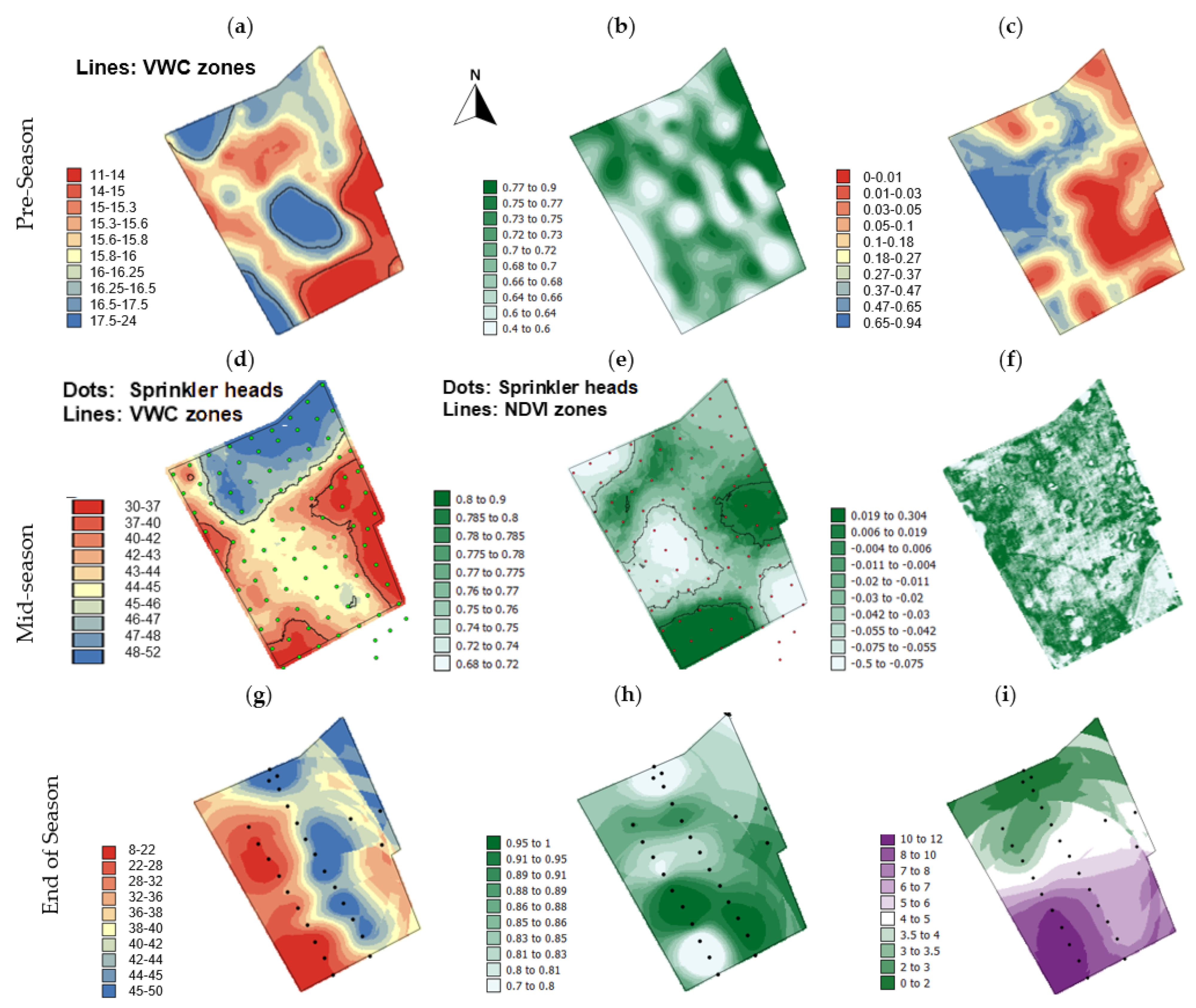
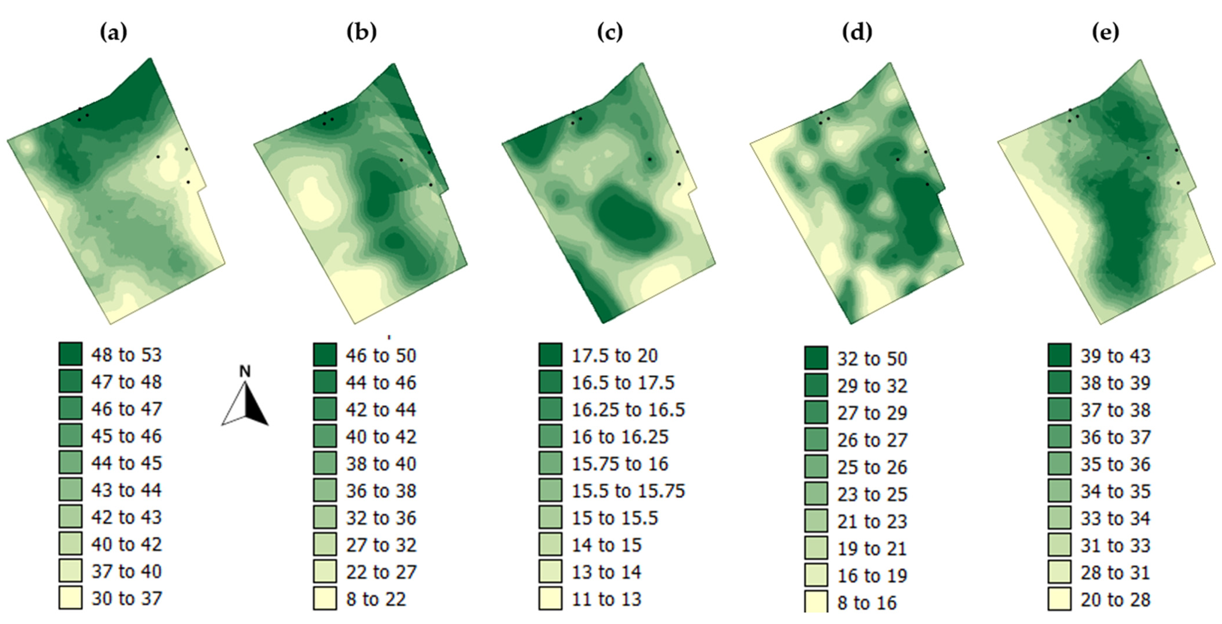
3.2. Temple Field—Spatial and Temporal Patterns

Typically, one would expect patterns of soil moisture in a field to be a function of patterns in topography and soil type or texture. The patterns of variation in the Temple field (Figure 7) do not seem to relate to patterns of variation in elevation (Figure 2c) which is not particularly surprising, given the unpredictable patterns of soil texture within this field. Straw et al. [38] also found that the strength of relationships between soil moisture and grass health patterns can vary between fields and with different soil types. Given the elevation patterns of the field, the unexpected dry areas at the base of the slope (western side of the field Figure 7d,g) could be related to the combination of the soil texture and the management practice of applying 30% less water to the three rows of sprinklers at the base of the slope in the 2021 growing season. Figure 7a shows that pre-season there are some wet and dry areas at the base of the slope, but by the mid- and end of the season (Figure 7d,f), the dry areas at the base of the slope become more pronounced due to management practice. The western edge of the field is next to the side-walk of a major road and pipes have been installed next to the sidewalk in the southern end of the field, with the soil probably being replaced by sand in these areas. This all suggests that managing the irrigation zones based on topography is not a good idea in this field.
There are some similarities in the patterns shown by the various variables observed for Temple field, but the similarities are generally a little less well defined than for Harmon field which is reflected in a slightly lower correlation coefficient between the variables (±0.1–0.6). The relationship between VWC and NDVI was found to be weakest for April 2022 during the period when the grass was emerging from winter dormancy. There are some similarities in the patterns of VWC for July 2021 (Figure 7d), in the middle of the irrigation season, and the VWC patterns for April 2022 (Figure 7a) before the irrigation season started. However, the relatively wet area in the central part of the field for April 2022 (Figure 7a) when the soil was generally very dry and under rainfed conditions corresponds with an area with low relative slope position, and the dry areas in the south and east of the field in April 2022 correspond with the top of the steepest slopes. This suggests that under natural conditions the soil moisture patterns may be more related to patterns of topography than when the field is irrigated. The larger area with higher VWC levels mid-irrigation-season (July 2021) than pre-irrigation-season (April 2022) could be related to the denser placement of sprinklers in the NE corner of the field (Figure 2c). The NE part of the field will become wetter when irrigated rather than when it is rainfed as it is receiving water from more sprinklers than other parts of the field (Figure 8c).
Unlike the Harmon field, the Temple field in July 2021 (mid-season) showed some of the greenest areas being associated with some of the driest locations such as in the SW corner and central eastern part of the field (Figure 7d,e). This suggests that there may be significant amounts of over-watering occurring in this field. The black lines on the maps in Figure 7d and e show the optimum zones developed using the kriged NDVI meter and % VWC data, respectively. The bivariate LMI between VARI data and VWC (Figure 8e) shows that the VWC zones essentially identify the significant spatial clusters of low–high areas (pale blue) where VARI is low, but VWC is high. These areas are probably receiving too much water. The two pale blue areas in the center of the field, with low VARI but high VWC, also correspond with areas of high foot traffic where sporting activities are concentrated, and excess water here could be increasing damage to the grass. The VWC zones also identify the significant spatial clusters of high–low values (pink) where VARI is high, but VWC is low. These areas suggest that the amount of water currently applied is sensible.
When the temporal patterns in VWC are examined for Temple field, the map for VWC with the greatest range in values (8–50% VWC) is Figure 7g for September 2021, this may reflect the after-effects of more-than-double the normal precipitation levels received in August 2021 followed by low precipitation levels in September, which could accentuate locations with differences in soil texture and thus soil water holding capacity. Figure 7a shows very dry soils throughout the Temple field before the 2022 irrigation season began (April 2022) with a range of only 13% in VWC values. In addition, the highest VWC values for April 2022 were less than the minimum values observed in July 2021.

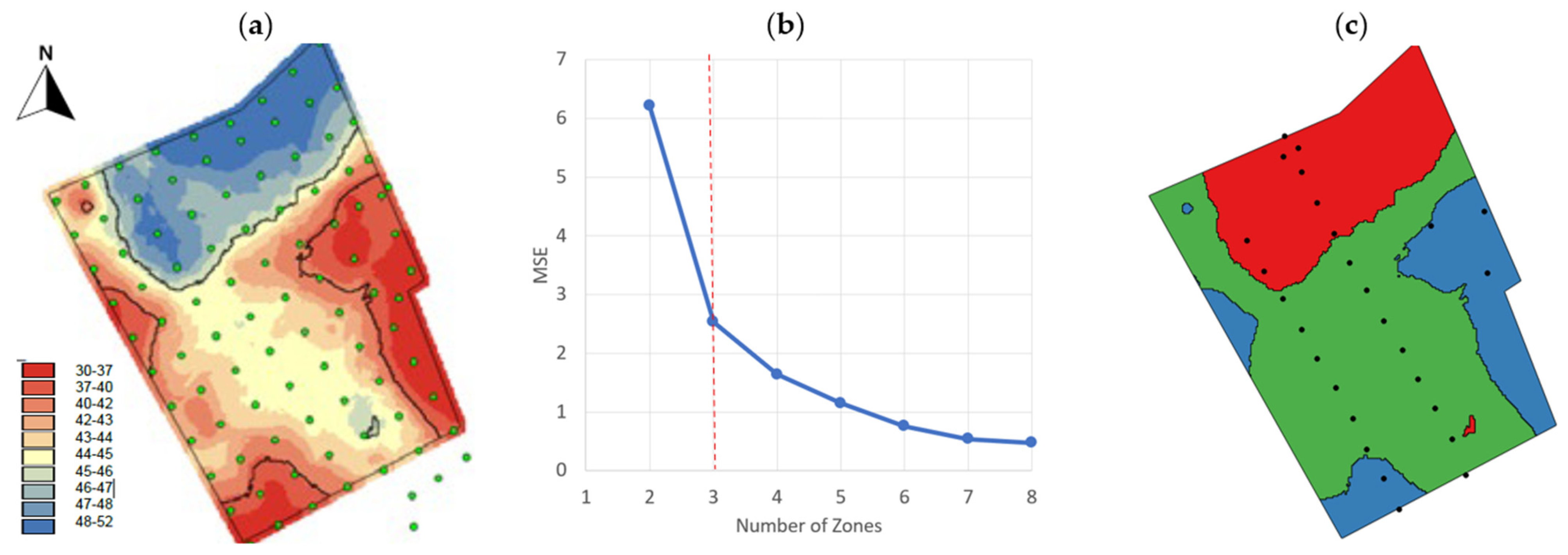
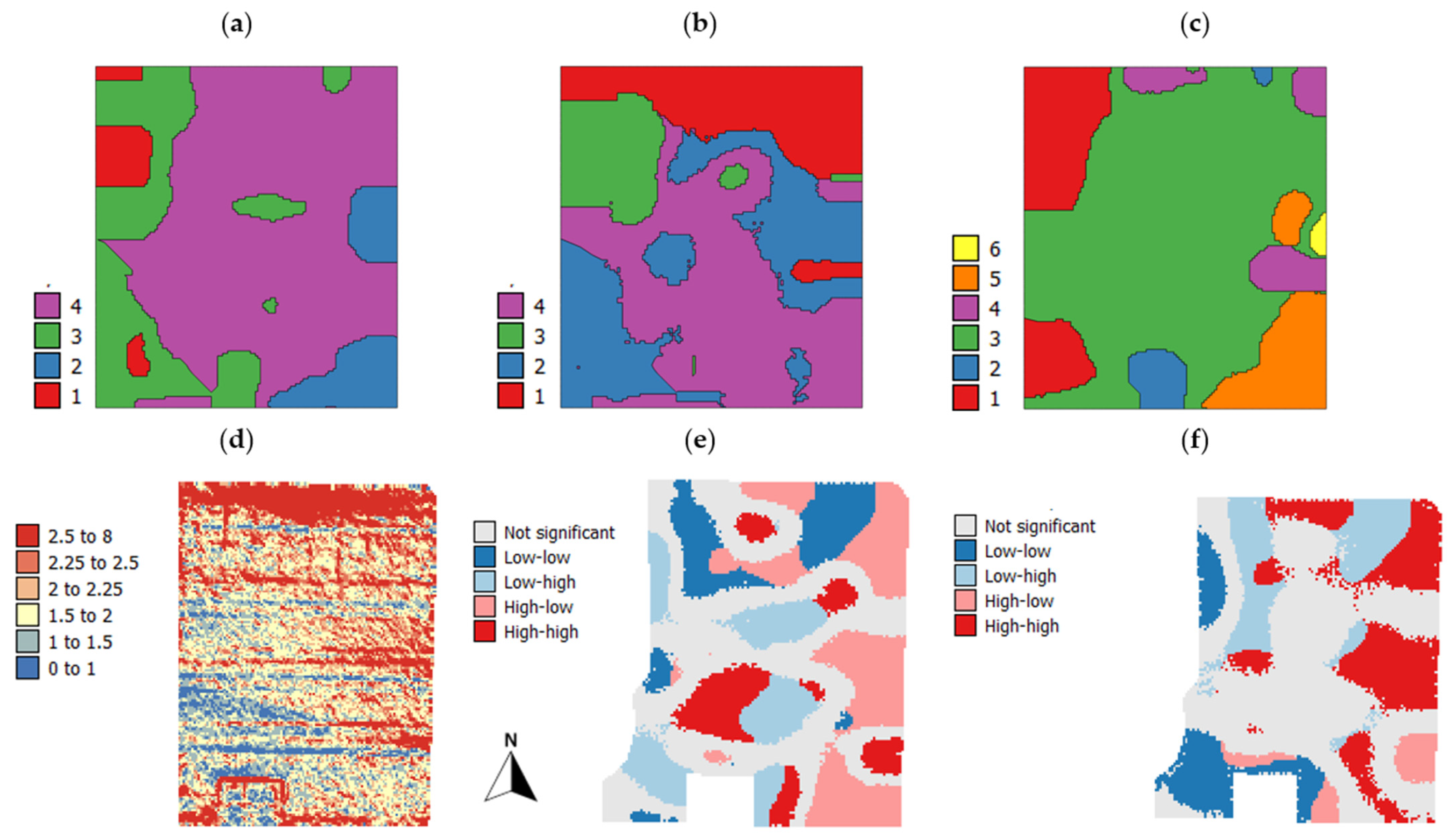
3.3. Harmon Field—Zones and Associated Errors

Figure 6a–c shows optimal zones for Harmon field created using different variables and from different time periods. The zones in the NW and the SE of the Harmon field in Figure 6a,c are consistent with the different soil types identified by the NRCS web soil survey (see black lines in Figure 5j). In addition, in each of these classifications, generally the large central area of the Harmon field is one class. Table 2 shows the summary statistics of the calculated absolute errors associated with treating the whole field as one zone, using existing zones and using optimal zones defined using different variables and all variables (including drone imagery and derived topographic attributes) combined. For Harmon field, when the field is treated as one zone or the zones are defined just by soil series, the mean absolute errors were generally larger than when other zones were used. This may be because the areas identified as having different soil series are confined to the NW and SE corners of the field (Figure 5j) and it is therefore very similar to using uniform irrigation and treating the whole field as one zone. Important errors, along with the mean absolute errors, is the range of absolute errors and their standard deviation. The range and standard deviation were generally largest, as might be expected, when the field was treated as one zone.
For Harmon field in the March 2021 pre-season sampling, the error (Table 2) was very small for the existing zones that cut across the main slope in line with elevation patterns (Figure 1c). This suggests, as does Figure 5a, that under rainfed conditions, the patterns of VWC largely reflect patterns in elevation and slope in this field and that spatially varying the irrigation rates with elevation is sensible with progressively less water being applied as the zones at the base of the slope are approached. For the other zones in the Harmon field for March 2021, the MAE was lowest for the zones defined using the wet/dry indicator; however, the range and standard deviation of errors was large. The best results overall were obtained from using the zones defined using March 2021 VWC as they had a low MAE, the smallest range and lowest standard deviation of errors. The worst performing zones pre-season based on MAE, range and standard deviation were the zones based on the March 2021 NDVI. The error statistics were worse for these zones than treating the whole field with uniform irrigation. This is probably due to the fact that when the grass is coming out of dormancy, the degree of greenness does not necessarily reflect soil VWC. Pre-season, of the free-to-measure variables (% dead grass and wet/dry indicator), the zones produced from dead grass patterns only performed slightly better than treating the whole field with uniform irrigation, but the wet/dry indicator zones had low errors.
For Harmon field in August 2021a, the mid-season survey, the MAE was lowest for existing zones, but the range and standard deviation of errors were both larger than zones based on some other variables. The next smallest MAEs were for zones based on August 2021a VWC and the August 2021a wet/dry indicator. The range and standard deviation of the errors were also smallest for August 2021a VWC followed by the wet/dry indicator. Zones based on the kriged NDVI meter, NDVI app values and dead grass percentages were similarly poorly performing in terms of MAEs, range, and standard deviation, and each had an MAE which was larger than that for managing the whole field uniformly as one zone. This shows that grass health is not just a function of VWC, but also varies with compaction, trafficking, and nutrient status of the soil; however, management practices often suggest that if there are brown patches of grass, the solution is to add more water. Indeed, at this within-season sampling we observed the turf mat being torn by mowers in areas that were particularly wet.
At the end of the irrigation season in Harmon field (September 2021) when patterns resulting from irrigation should be most defined, the VWC zones were the best-performing according to the minimum, maximum, and standard deviation of the absolute errors (Table 2). The results for Harmon field showed that after the VWC zones for the same date, VWC zones based on all survey dates performed next best followed by wet/dry zones from September 2021. For the end of the irrigation season, existing zones performed well in terms of MAE but not in terms of the range of errors. The zones based on NDVI or all variables from September 2020 performed slightly better than treating the whole field as one zone in terms of MAE, range and standard deviation. This could possibly be linked to the high level of detail in the drone data as they were not interpolated by kriging, which is a smoothing process which can lead to more spatially coherent zones with less random variation. The NDVI measurements being more useful for defining zones at the end of the season rather than pre- or mid-season makes sense as the patterns in grass response to areas that have been well-, over- and under-watered during the season are likely to be most pronounced. However, the fact that zones based on NDVI measurements only become slightly useful at the end of the season suggests they should generally not be used. For all surveys in the Harmon field, zones based on the wet/dry indicator performed better than the NDVI meter measurements, suggesting that residential customers may be able to determine when different zones need watering by merely touching or looking at the topsoil to see if it looks or feels wet or dry at several places in each zone. However, this method can only work for mapping in a large field if the whole field, or a very large percentage of it, is not universally wet or dry.
As VWC zones were the best-performing pre-, mid-, and at the end of the season for Harmon field, the last two rows in Table 2 show how using VWC zones from a different survey perform for this field. Using March 2021 zones to manage VWC in August 2021 would have produced errors that were slightly larger, but with similar characteristics to the August 2021 wet/dry zones. The August 2021 zones performed less well with the Mar21 VWC data, but these results suggest that it may be possible to use temporally stable zones for this field that are based on VWC. In addition, the good performance of the wet/dry indicators zones suggests that very cheap, crude soil moisture sensors could be installed in the field to determine when each zone should be watered.

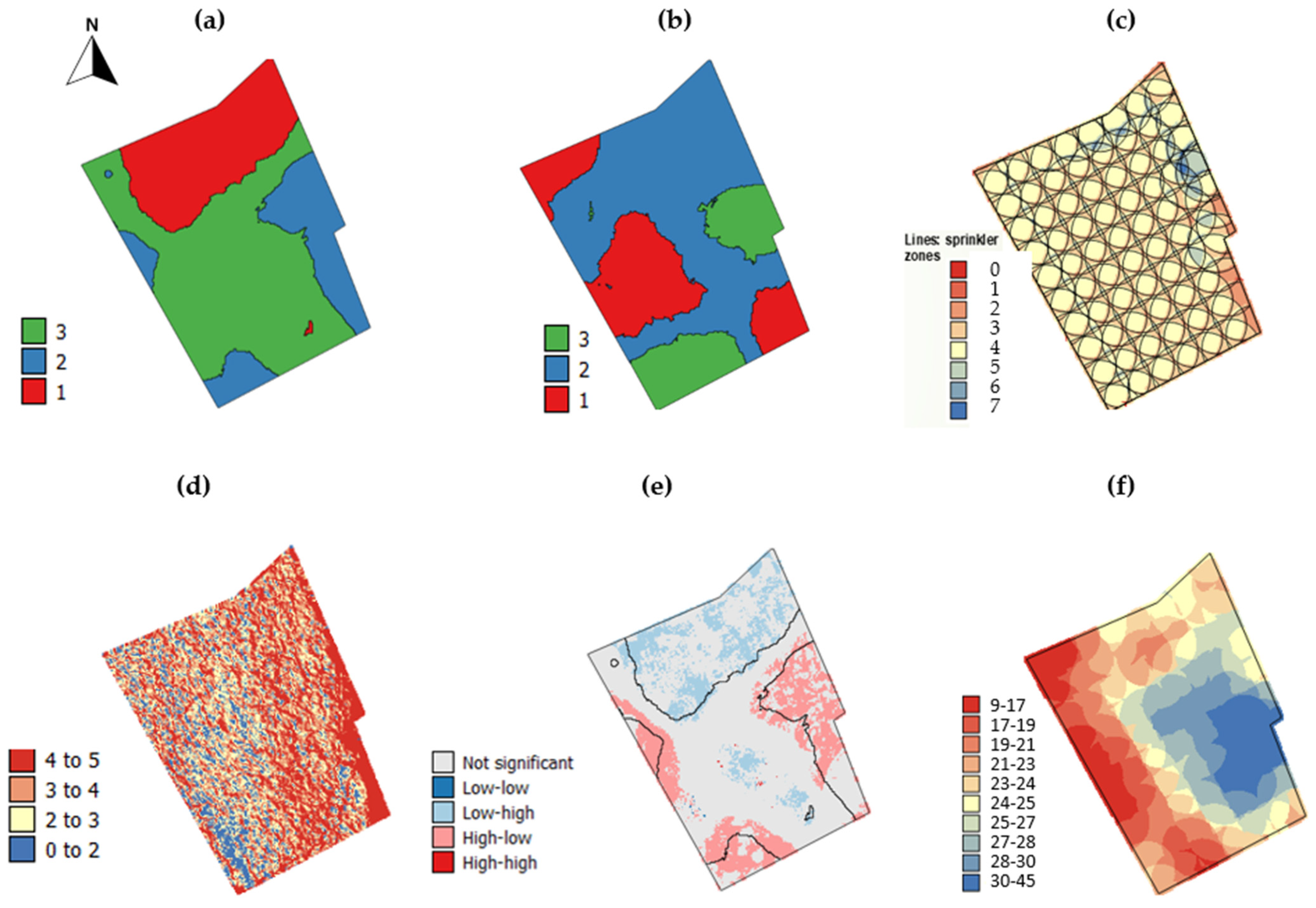
3.4. Temple Field—Zones and Associated Errors

Figure 8a,b show examples of zones for Temple field that are based on VWC and NDVI values from July 2021. For Temple field in April 2022, during the pre-season survey, the range and standard deviation of the absolute errors showed that zones based on the wet/dry indicator, all variables (including drone vegetation indices and derived topographic attributes), dead grass, and NDVI all performed similarly to each other and similarly to when treating the whole field as one zone (Table 3). This is likely because in April 2022 the whole field was very dry (VWC 11–24%) and there was not much variation in VWC within the field, therefore the errors were small for all approaches.
The best-performing type of zones was existing zones, namely if the VWC values were averaged within the 27 m radius around each sprinkler head, and also in the areas of overlap between sprinkler heads. However, they are very small and have never been managed individually to date. Figure 8f shows for May 2022 the average VWC per sprinkler zone, and that this is a very complicated pattern to implement and would involve calculations about what to do for the zones that are in areas of overlap between different sprinkler heads (Figure 8c). This is also complicated by the northeast edges of the field where the sprinkler spacing is slightly different. For April 2022, the best performing zones based on MAE, range, and standard deviation of errors were the zones based on April 2022 VWC.
Figure 8. Maps showing the configuration of zones for Temple Field based on (a) VWC zones (July 2021) and (b) NDVI zones (July 2021)), (c) sprinkler impact number (d) Slope (°) from drone DSM, (e) LMI for VARI and VWC (July 2021), and (f) average VWC per sprinkler zone (May 2022).
Agronomy 13 01267 g008
In the Temple field mid-season survey (July 2021), the errors (Table 3) show that, like Harmon field, zones based on VWC values (Figure 7d) are more effective than NDVI zones (Figure 7e). This makes sense as there are several other factors that can affect grass greenness other than VWC such as nutrient levels, soil texture, and compaction. The VWC zones being better than NDVI-based zones mid-season is also confirmed by the bi-variate LMI analysis of VARI and VWC (Figure 8e), which showed that the VWC zones identify the wettest and driest zones well and that the LMI analysis can help determine which zones are being over- or under-watered and thus need either more or less water. Although the VWC zones have larger errors than using each sprinkler head as its own zone, implementing use of these zones would be far simpler than calculating how much water to apply to each individual sprinkler head for each irrigation event.
The errors for Temple field in April 2022 for all types of zones are at least an order of magnitude smaller than for July 2021. In April 2022, the field was very dry and thus the range of VWC values was small compared to July 2021 (compare Figure 7a and Figure 7d). This resulted in the range and standard deviation of the absolute errors being smaller for April 2022 than July 2021. The end-of-season September 2021 zones for Temple field (Table 3) showed that all variables performed better than treating the whole field as one zone in terms of all error criteria; however, zones based on NDVI and dead grass were the worst performing and VWC zones the best. Unfortunately, it was not possible to produce a meaningful wet/dry indicator map and associated zones for this survey. As can be seen for the deciles map (Figure 7g), only 10% of the soil in the field had VWCs < 20% and as the dry locations were quite randomly located, it was not possible to produce a map for the wet/dry indicator in September 2021.
As VWC-based zones were the best-performing pre-, mid- and at the end of the season for both Harmon and Temple fields, the last five rows in Table 3 show how using VWC zones from a different survey performed for Temple field. Generally, using zones from another time produced low errors, but the range and standard deviation of the errors was large when May 2022 VWC zones were used with September 2021 VWC values and September 2021 VWC zones were used with May 2022 VWC values. While there are similarities in the patterns of VWC between different surveys for the Temple field, they are less consistent than the patterns for the Harmon field and are not particularly related to broad patterns in elevation. This is probably a result of the more densely packed sprinklers at the top of the slope and sandy soil at the bottom of the slope due to pipeline installation along the side-walk. All surveys basing zones on NDVI performed similarly to treating the whole field like one zone and having uniform irrigation, so this should be avoided. This shows that there is not always a positive relationship between NDVI and soil moisture, and others have found negative relationships between NDVI and soil moisture in certain locations [39].
As VWC zones were the best-performing for both fields, apart from existing zones in Temple field that could not be practically managed without detailed spatial information, Figure 9 and Figure 10 show maps of VWC for both fields on all survey dates. As mentioned earlier, for Harmon field, both an E–W pattern and a N–S pattern are evident with the latter being slightly stronger for the VWC data than the NDVI data (Figure 5b,e,h,k). The N–S pattern is most pronounced for March 2021, which was before the start of the irrigation season, and is likely to reflect the natural, long-term soil moisture patterns under rainfed conditions. The curved black lines in Figure 9 show the zones based on the March 2021 VWC and how they relate to patterns in VWC levels from other surveys. Clearly, from the legends of the maps in Figure 9, the range of % VWC in the field changes over time but there is a general pattern of the southerly five zones (below the red dashed line) having larger % VWC than the northerly zones. Indeed, the black dots show the locations of sensors that have been installed in this field which could help determine the amount of water needed in these two sets of existing zones and could also determine if irrigation rates should be varied within the northerly and southerly zones, as there are sensors within two of the northerly and two of the southerly zones.
Temple field patterns in VWC for all surveys are less consistent than for Harmon field, but all surveys apart from that for July 2021 seem to have areas with larger VWCs in the center of the field and all surveys apart from May 2022 have some areas with large VWCs in the north end of the field. Given the slightly less consistency in the spatial patterns of VWC in this field, but the general good performance of the wet/dry indicator survey, it suggests that rather than having sensors limited to areas that were identified as generally wet and dry in the July 2021 survey (see sensor locations at the end of the northerly transect and on the eastern edge of the field in Figure 4c), it would be a good idea to install multiple inexpensive and less accurate soil moisture sensors to determine broad patterns of wet/dryness before irrigation events. There is also a lot more potential in this field to control the spatial patterns of water application given that valve-in-head sprinkler heads are installed in it.
The total water used in the 2022 season to irrigate the Harmon field was 8,066,754 gallons, and 18,241,055 gallons were used in Temple field. Estimations have been made that these huge volumes of water could be reduced by as much as 50% if effective spatial zones were implemented [9] or if sub-surface drip irrigation directed by calculations of crop water stress index from infra-red thermometer surveys were used [10]. Either approach could result in huge water savings for institutions such as Brigham Young University when multiplied over all irrigation zones for the whole campus; however, the relative cost of sensing/survey to inform spatial zones needs to be balanced against the water savings possible.

4. Conclusions

This analysis demonstrates that a lot more control is possible over where spatial zones are with valve-in-head sprinkler heads, and thus less water can be wasted. However, analysis for the Harmon field which does not have valve-in-head sprinklers shows that even adjusting irrigation rates applied to existing zones can save water. The results of this study suggest that sprinkler zones for irrigation of turfgrass in large general-purpose sports fields are best determined through spatial surveys of soil moisture rather than surveys of several different variables or by NDVI and other measures of grass health. Patterns of grass health seem to become more accentuated by the end of the season and the errors for both fields showed that zones based on NDVI were only slightly more useful than uniform irrigation by the end of the season. As field managers generally observe the grass health rather than the soil moisture and assume that brown spots are the result of lack of water, the causes of areas with poor grass health, such as excess compaction in the west of the Harmon field, need to be determined to help field managers to change their watering practices.
Both fields used in this analysis suggest that patterns in VWC change temporally and that it would be best to redefine spatial irrigation zones periodically. However, this would require significant investment in automated sensing and mapping equipment that could communicate with a smart sprinkler system. It could also be prohibitively expensive given that no crop is produced for sale by turfgrass that can offset the price of survey and sensing equipment. However, given that the wet/dry indicator zones performed second-best in most surveys, yet the method requires no purchase of equipment and is therefore the cheapest method used, it seems that the spatial configuration of zones could be based on patterns in soil moisture from one or a few surveys and that the timing of irrigation events could be determined by field managers touching the soil at several locations in each zone to determine if it feels wet or dry. Another alternative is that timing of irrigation could be determined by the placement of very inexpensive but less-accurate sensors in each irrigation zone. In addition, given that there are similarities in the patterns of VWC over time that relate to patterns of slope and soil texture, and that using VWC zones data from all sampling times or from another time period performed better than using NDVI zones, sensible approaches to static zoning would be basing zones on an average of VWC values from several surveys taken at different times within the season, or on soil moisture levels before the irrigation season starts (e.g., March 2021 for Harmon field and April 2022 for Temple field) when the patterns are more reflective of permanent field characteristics such as topography and soil texture.
The patterns of variation in VWC for the Harmon field were more consistent over time than those for the Temple field and related well to patterns of relative elevation. Given this, and the ability to have more control over the spatial patterns of irrigation in the Temple field with the valve-in-head sprinkler heads, an inexpensive method for frequently mapping VWC in this field is needed. The ability of EM38 surveys to identify zones within turfgrass fields and determine their consistency should be evaluated as these are relatively swift non-invasive surveys which have proved useful in determining zones for various aspects of precision agriculture, given the frequent relationship to soil texture and soil moisture. Consulting firms could determine zones using such equipment just once per location before the irrigation season starts to characterize differences in VWC that are likely due to permanent features of the soil, such as texture and topography, rather than management effects. Another possibility to investigate in the future is drought indices, such as the crop water stress index from thermal IR drone imagery, to determine if the same locations are consistently experiencing water deficit throughout the irrigation season. The final question that needs addressing is that once irrigation rates are modified to fit the optimal zones that are defined, will the management effect of varying rates between zones significantly affect the spatial patterns in soil moisture? If so, this would mean that zones need to be constantly re-defined, making it imperative to find inexpensive, automated ways of sensing soil moisture patterns.

Author Contributions

Conceptualization, R.K., N.C.H. and B.G.H.; methodology, R.K., K.H., S.R.S., D.G., S.S. and R.R.J.; software, R.K., B.I. and S.R.S.; validation, R.K., B.I. and S.R.S.; formal analysis, R.K., B.I. and S.S.; investigation, R.K., B.I., K.H., S.R.S., D.G., R.R.J., S.S., N.C.H. and B.G.H.; resources, R.K., R.R.J., S.S., N.C.H. and B.G.H.; writing—original draft preparation, R.K., B.I. and R.R.J.; writing—review and editing, R.K., B.I., K.H., S.R.S., D.G., R.R.J., S.S., N.C.H. and B.G.H.; visualization, R.K., B.I. and S.R.S.; supervision, R.K., B.I., R.R.J., N.C.H. and B.G.H.; project administration, R.K.; funding acquisition, R.K. and B.G.H. All authors have read and agreed to the published version of the manuscript.

Funding

This research was funded by The Redd Center for Western Studies at Brigham Young University, who provided some funding towards this research, and the College of Family Home and Social Sciences purchased the sensors installed in the fields and funded student research through the experiential learning fund.

Data Availability Statement

Interested parties can contact the corresponding author regarding data availability.

Acknowledgments

Dave Hawks of the BYU Grounds crew provided assistance and insights to field work as well as information on total water applied to the field sites in 2022. Several students not listed as authors assisted with more than one of the field surveys that this paper is based on: Connor Golden, Sophia Harris, Abigail Henrie, Austen Lambert, Autumn Lee, Alexandra Olsen, Kirsten Sanders, Autumn Welling, Christian Ybanez.

Conflicts of Interest

The authors declare no conflict of interest.

References

  1. Anderson, M.T.; Woosley, L.H. Water Availability for the Western United States—Key Scientific Challenges; USGS: Reston, VA, USA, 2005.
  2. Milesi, C.; Running, S.W.; Elvidge, C.D.; Dietz, J.B.; Tuttle, B.T.; Nemani, R.R. Mapping and Modeling the Biogeochemical Cycling of Turf Grasses in the United States. Environ. Manag. 2005, 36, 426–438. [Google Scholar] [CrossRef] [PubMed]
  3. EPA. Keeping Your Cool: How Communities Can Reduce the Urban Heat Island Effect; EPA: Washington, DC, USA, 2014.
  4. Wood, R.A.; Burchett, M.D.; Alquezar, R.; Orwell, R.L.; Tarran, J.; Torpy, F. The Potted-Plant Microcosm Substantially Reduces Indoor Air VOC Pollution: I. Office Field-Study. Water Air Soil Pollut. 2006, 175, 163–180. [Google Scholar] [CrossRef]
  5. Gibbons, P.; Gill, A.M.; Shore, N.; Moritz, M.A.; Dovers, S.; Cary, G.J. Options for Reducing House-Losses during Wildfires without Clearing Trees and Shrubs. Landsc. Urban Plan. 2018, 174, 10–17. [Google Scholar] [CrossRef]
  6. Fisher, M.J.; Rao, I.M.; Ayarza, M.A.; Lascano, C.E.; Sanz, J.I.; Thomas, R.J.; Vera, R.R. Carbon Storage by Introduced Deep-Rooted Grasses in the South American Savannas. Nature 1994, 371, 236–238. [Google Scholar] [CrossRef]
  7. Dass, P.; Houlton, B.Z.; Wang, Y.; Warlind, D. Grasslands May Be More Reliable Carbon Sinks than Forests in California. Environ. Res. Lett. 2018, 13, 074027. [Google Scholar] [CrossRef]
  8. Beard, J.B.; Green, R.L. The Role of Turfgrasses in Environmental Protection and Their Benefits to Humans. J. Environ. Qual. 1994, 23, 452–460. [Google Scholar] [CrossRef] [Green Version]
  9. EPA. Water Efficiency Management Guide: Landscaping and Irrigation; EPA 832-F-17-016b; EPA: Washington, DC, USA, 2017.
  10. Orta, A.H.; Todorovic, M.; Ahi, Y. Cool- and Warm-Season Turfgrass Irrigation with Subsurface Drip and Sprinkler Methods Using Different Water Management Strategies and Tools. Water 2023, 15, 272. [Google Scholar] [CrossRef]
  11. Liakos, V.; Vellidis, G. Sensing with Wireless Sensor NetworksWireless Sensor Networks (WSNs). In Sensing Approaches for Precision Agriculture; Kerry, R., Escolà, A., Eds.; Progress in Precision Agriculture; Springer International Publishing: Cham, Switzerland, 2021; pp. 133–157. ISBN 978-3-030-78431-7. [Google Scholar]
  12. O’Shaughnessy, S.A.; Evett, S.R.; Colaizzi, P.D. Dynamic Prescription Maps for Site-Specific Variable Rate Irrigation of Cotton. Agric. Water Manag. 2015, 159, 123–138. [Google Scholar] [CrossRef]
  13. Straw, C.M.; Henry, G.M. Spatiotemporal Variation of Site-Specific Management Units on Natural Turfgrass Sports Fields during Dry Down. Precis. Agric. 2018, 19, 395–420. [Google Scholar] [CrossRef]
  14. Straw, C.M.; Grubbs, R.A.; Tucker, K.A.; Henry, G.M. Handheld versus Mobile Data Acquisitions for Spatial Analysis of Natural Turfgrass Sports Fields. HortScience 2016, 51, 1176–1183. [Google Scholar] [CrossRef]
  15. Straw, C.M.; Henry, G.M.; Shannon, J.; Thompson, J.J. Athletes’ Perceptions of within-Field Variability on Natural Turfgrass Sports Fields. Precis. Agric. 2019, 20, 118–137. [Google Scholar] [CrossRef]
  16. Rybka, K.; Żurek, G.; Wolski, K. Turfgrass Simulation for Increased Performance in Changing Climate, Special issue. Agronomy 2022, 12. Available online: https://www.mdpi.com/journal/agronomy/special_issues/turfgrass_climate#Other (accessed on 14 March 2023).
  17. Xu, Y.; Wang, K.; Zhang, J.; Xia, C.; Liu, T. Advances in Stress Biology of Forage and Turfgrass, Special issue. Agronomy 2023, 12–13. Available online: https://www.mdpi.com/journal/agronomy/special_issues/D2VQ9R88RM (accessed on 14 March 2023).
  18. Huff, D.R. Turfgrass Biology, Genetics, and Breeding, Special issue. Agronomy 2018, 8. Available online: https://www.mdpi.com/journal/agronomy/special_issues/turfgrass_biology (accessed on 14 March 2023).
  19. Zhang, W.; Yu, J. Advances in Genetics, Breeding, and Quality Traits in Forage and Turf Grass, Special issue. Agronomy 2023, 12–13. Available online: https://www.mdpi.com/journal/agronomy/special_issues/genetics_grass (accessed on 14 March 2023).
  20. Webster, R.; Oliver, M.A. Sample Adequately to Estimate Variograms of Soil Properties. J. Soil Sci. 1992, 43, 177–192. [Google Scholar] [CrossRef]
  21. Spectrum Technologies Inc. FieldScout GreenIndex+ Turf Product Manual Item # 2910TA, 2910T; Spectrum Technologies Inc.: Aurora, IL, USA, 2014. [Google Scholar]
  22. Conrad, O.; Bechtel, B.; Bock, M.; Dietrich, H.; Fischer, E.; Gerlitz, L.; Wehberg, J.; Wichmann, V.; Böhner, J. System for Automated Geoscientific Analyses (SAGA) v. 2.1.4. Geosci. Model Dev. 2015, 8, 1991–2007. [Google Scholar] [CrossRef] [Green Version]
  23. Anselin, L. Local Indicators of Spatial Association—LISA. Geogr. Anal. 1995, 27, 93–115. [Google Scholar] [CrossRef]
  24. Vitharana, U.W.A.; Van Meirvenne, M.; Simpson, D.; Cockx, L.; De Baerdemaeker, J. Key Soil and Topographic Properties to Delineate Potential Management Classes for Precision Agriculture in the European Loess Area. Geoderma 2008, 143, 206–215. [Google Scholar] [CrossRef]
  25. Khosla, R.; Inman, D.; Westfall, D.G.; Reich, R.M.; Frasier, M.; Mzuku, M.; Koch, B.; Hornung, A. A Synthesis of Multi-Disciplinary Research in Precision Agriculture: Site-Specific Management Zones in the Semi-Arid Western Great Plains of the USA. Precis. Agric. 2008, 9, 85–100. [Google Scholar] [CrossRef]
  26. Monroe, J.G.; Cai, H.; Des Marais, D.L. Diversity in Nonlinear Responses to Soil Moisture Shapes Evolutionary Constraints in Brachypodium. G3 Genes Genomes Genet. 2021, 11, jkab334. [Google Scholar] [CrossRef]
  27. Xu, Z.; Zhou, G. Responses of Photosynthetic Capacity to Soil Moisture Gradient in Perennial Rhizome Grass and Perennial Bunchgrass. BMC Plant Biol. 2011, 11, 21. [Google Scholar] [CrossRef] [Green Version]
  28. Engstrom, R.; Hope, A.; Kwon, H.; Stow, D. The Relationship between Soil Moisture and NDVI Near Barrow, Alaska. Phys. Geogr. 2008, 29, 38–53. [Google Scholar] [CrossRef]
  29. Kerry, R.; Ingram, B.; Orellana, M.; Ortiz, B.V.; Scully, B. Development of a Method to Assess the Risk of Aflatoxin Contamination of Corn within Counties in Southern Georgia, USA Using Remotely Sensed Data. Smart Agric. Technol. 2023, 3, 100124. [Google Scholar] [CrossRef]
  30. Mahmoudzadeh, H.; Matinfar, H.R.; Kerry, R.; Eskandari, S.; Ebrahimi-Khusfi, Z.; Taghizadeh-Mehrjardi, R. New Hybrid Evolutionary Models for Spatial Prediction of Soil Properties in Kurdistan. Soil Use Manag. 2022, 38, 191–211. [Google Scholar] [CrossRef]
  31. Abedi, F.; Amirian Chakan, A.; Faraji, M.; Taghizadeh, R.; Kerry, R.; Razmjoue, D.; Scholten, T. Salt Dome Related Soil Salinity in Southern Iran: Prediction and Mapping with Averaging Machine Learning Models. Land Degrad. Dev. 2021, 32, 1540–1554. [Google Scholar] [CrossRef]
  32. Mahmoudzadeh, H.; Matinfar, H.R.; Taghizadeh-Mehrjardi, R.; Kerry, R. Spatial Prediction of Soil Organic Carbon Using Machine Learning Techniques in Western Iran. Geoderma Reg. 2020, 21, e00260. [Google Scholar] [CrossRef]
  33. Fathizad, H.; Ardakani, M.A.H.; Sodaiezadeh, H.; Kerry, R.; Taghizadeh, R. Investigation of the Spatial and Temporal Variation of Soil Salinity Using Random Forests in the Central Desert of Iran. Geoderma 2020, 365, 114233. [Google Scholar] [CrossRef]
  34. Nawaz, M.F.; Bourrié, G.; Trolard, F. Soil Compaction Impact and Modelling. A Review. Agron. Sustain. Dev. 2013, 33, 291–309. [Google Scholar] [CrossRef] [Green Version]
  35. Shaheb, M.R.; Venkatesh, R.; Shearer, S.A. A Review on the Effect of Soil Compaction and Its Management for Sustainable Crop Production. J. Biosyst. Eng. 2021, 46, 417–439. [Google Scholar] [CrossRef]
  36. Avoid Overwatering Lawns & Landscapes, Nebraska Drought Resources, Nebraska. Available online: https://droughtresources.unl.edu/avoid-overwatering-lawns-landscapes (accessed on 19 April 2023).
  37. Ruiz, A.M.; Furtado, E.; Pieroni, L.; Albuquerque, F. Use of Multispectral Images for Identifying Overwatering in Eucalyptus Plantation. In Proceedings of the XXV IUFRO World Congress 2019, Curitiba, Brazil, 29 September–5 October 2019. [Google Scholar]
  38. Straw, C.M.; Grubbs, R.A.; Henry, G.M. Short-Term Spatiotemporal Relationship between Plant and Soil Properties on Natural Turfgrass Sports Fields. Agrosyst. Geosci. Environ. 2020, 3, e20043. [Google Scholar] [CrossRef] [Green Version]
  39. Felegari, S.; Sharifi, A.; Moravej, K.; Golchin, A.; Tariq, A. Investigation of the Relationship between NDVI Index, Soil Moisture, and Precipitation Data Using Satellite Images. In Sustainable Agriculture Systems and Technologies; John Wiley & Sons, Ltd.: Hoboken, NJ, USA, 2022; pp. 314–325. ISBN 978-1-119-80856-5. [Google Scholar]
Figure 1. Maps of Harmon field showing (a) 15 m ground survey grid (15 m grid, ground survey points, and soil series boundaries (black lines)), (b) September 2020 RGB Drone image degraded to 1 m pixel size, (c) Sprinkler zones in relation to elevation (m) (Sprinkler zones (black lines) and elevation from 1387 m (blue) to 1392 m (red). Black dots: transect survey points from September 2021 soil texture survey.).
Agronomy 13 01267 g001
Figure 2. Maps of Temple field showing (a) ground survey grid (15 m grid, ground survey points), (b) July 2021 RGB drone image, sports equipment shed indicated by star, and (c) Sprinkler heads (black dots) and zones (black lines) in relation to elevation (m) from 1443 m (blue) to 1463 m (red) and arrow indicates area of high density of sprinkler heads.
Agronomy 13 01267 g002
Figure 3. Climograph for Provo, Utah showing 30-year normal and Actual Monthly Rainfall and Average Temperatures for 2020–2022.
Agronomy 13 01267 g003
Figure 4. Maps and graph of Temple field showing (a) kriged VWC (%) within the field with sprinkler heads (green dots) and proposed VWC zones (black lines), (b) scree plot for determining optimal number of zones, and (c) location of 3 optimal zones based on July 2021 VWC (Zone 1: blue, low VWC; Zone 2: green, medium VWC; Zone 3: red, high VWC. Black dots are September 2021 transect survey and sensor locations).
Agronomy 13 01267 g004
Figure 5. Maps of Harmon Field for: (a) % VWC (March 2021), (b) NDVI (March 2021), (c) Dead grass (March 2021), (d) % VWC (August 2021a), (e) NDVI (August 2021a), (f) Wet/Dry Indicator (IND) (August 2021a), (g) % VWC (September 2020), (h) NDVI (September 2020), (i) Dead grass (September 2020), (j) % VWC (September 2021), (k) NDVI (September 2021), and (l) Wet/Dry Indicator (September 2021).
Agronomy 13 01267 g005
Figure 6. Maps showing the configuration of zones for Harmon Field (ac) based on different variables: (a) Harmon field VWC zones (September 2020), (b) Harmon field all variables zones (March 2021), (c) Harmon field all dates VWC zones, and maps of (d) slope (°) from drone DSM, (e) LMI for VWC and dead grass (September 2020), and (f) LMI for VWC and NDVI meter (September 2020).
Agronomy 13 01267 g006
Figure 7. Maps of Temple Field for: (a) % VWC (April 2022), (b) NDVI (April 2022), (c) Wet/Dry indicator (IND) (April 2022), (d) % VWC (July 2021), dots are sprinkler heads and lines are VWC zones (e) NDVI (July 2021), dots are sprinkler heads and lines are NDVI zones, (f) drone VARI (July 2021), (g) % VWC (September 2021), (h) NDVI (September 2021), and (i) dead grass (September 2021), dots in (gi) show September 2021 sample points and sensor locations.
Agronomy 13 01267 g007
Figure 9. Maps of % VWC for Harmon field for (a) September 2020, (b) March 2021, (c) August 2021a, (d) August 2021b, and (e) September 2021. (Black Straight lines show existing sprinkler zones, black curved lines show March 2021 soil moisture zones, black dots show locations of soil moisture sensors and data loggers, and red dotted line shows the divide between wetter zones towards the base of the slope and drier zones at the top of the slope).
Agronomy 13 01267 g009
Figure 10. Maps of % VWC for Temple field for (a) July 2021, (b) September 2021, (c) April 2022, (d) May 2022, and (e) October 2022. (Black dots show locations of soil moisture sensors and data loggers).
Agronomy 13 01267 g010
Table 1. Summary of Variables Measured, Instruments Used and Dates Sampled for Field and Drone Surveys of Harmon and Temple fields. (a and b refer to first and second of two surveys in August 2021).
VariableMethod or Instrument UsedHarmon Sampling DatesTemple Sampling Dates
% dead or discolored grassEstimates using quadratsSeptember 2020, March 2021, August 2021a, September 2021September 2021, April 2022
Soil Dry/Wet (0/1) IndicatorTouchSeptember 2020, March 2021, August 2021a+b, September 2021April 2022
NDVI meterTrimble GreenSeeker handheldSeptember 2020, March 2021, August 2021a+b, September 2021July 2021, September 2021, April 2022, May 2022
NDVI AppFieldScout GreenIndex+ Turf app and board [21]August 2021a+b, September 2021July 2021, April 2022
Top-soil VWC (%)Delta T theta probeSeptember 2020, March 2021, August 2021a+b, September 2021September 2021, July 2021, April 2022, May 2022
Elevation (m) (6 cm pixels)
and Slope, Aspect, TWI
Drone DSM processed in Drone Deploy, Pix4D then SAGA GIS [22]September 2020, March 2021, August 2021July 2021, April 2022
R, G, B, NIR, NDVI, VARI
(2 cm and 6 cm pixels)
Drone images processed in Drone Deploy and Pix4DSeptember 2020, March 2021, August 2021July 2021, April 2022
Table 2. Summary statistics of absolute errors between kriged VWC (Harmon, March 2021, August 21a, September 2021) and average VWC per field or zone based on zones calculated with different variables and combinations of variables.
VWC Data Used and Zone TypeMeanMin.Max.St. Dev.
Pre-seasonHarmon March 2021—whole field zone0.0049−16.5314.775.72
Harmon March 2021—existing zones2.4271 × 10−14−20.3111.423.76
Harmon March 2021—March 2021 VWC zones0.0048−9.3408.522.33
Harmon March 2021—March 2021 Dead grass zones0.0046−15.0315.725.55
Harmon March 2021—March 2021 NDVI zones0.0063−16.5916.385.26
Harmon March 2021—March 2021 Wet/Dry zones2.8140 × 10−6−18.9413.655.35
Mid-seasonHarmon August 2021—whole field zone0.0138−9.919.723.42
Harmon August 2021—existing zones5.3652 × 10−15−13.297.602.72
Harmon August 2021—August 2021 VWC zones0.0015−5.612.880.99
Harmon August 2021—August 2021 Dead grass zones0.0161−7.748.423.08
Harmon August 2021—August 2021 NDVI zones0.0149−9.869.373.27
Harmon August 2021—August 2021 NDVI app zones0.0130−9.839.963.35
Harmon August 2021—August 2021 Wet/Dry zones0.0086−8.917.422.63
End of SeasonHarmon September 2021—whole field 1 zone0.0060−11.5412.34.23
Harmon September 2021—existing zones2 × 10−10−16.8310.683.38
Harmon September 2021—September 2021 VWC zones9.402 × 10−7−5.346.001.63
Harmon September 2021—All dates VWC zones6.62 × 10−7−8.168.332.64
Harmon September 2020—September 2020 NDVI zones0.0001−11.6812.334.17
Harmon September 2021—September 2021 Wet/Dry zones1.7661 × 10−6−9.8210.493.8
Harmon September 2021—Soil Series zones3.93−15.3119.774.95
Harmon September 2020—September 2020 All Variables zones1.0915 × 10−6−10.5213.293.98
VWC zones other timesHarmon August 2021—March 2021 VWC zones0.0091−8.868.642.76
Harmon March 2021—August 2021 VWC zones4.5936−12.57−1.801.53
Table 3. Summary statistics of absolute errors between kriged VWC (Temple, April 2022, July 2021 and September 2021) and average VWC per field or zone based on zones calculated with different variables and combinations of variables.
VWC Data Used and Zone TypeMeanMin.Max.St. Dev.
Pre-seasonTemple April 2022—whole field 1 zone0.0829−4.087.381.46
Temple April 2022—existing zones3.035 × 10−5−1.874.060.59
Temple April 2022—April 2022 VWC zones0.0829−1.895.290.69
Temple April 2022—April 2022 dead grass zones0.0829−3.937.161.40
Temple April 2022—April 2022 NDVI zones0.0830−4.347.071.40
Temple April 2022—April 2022 wet/dry zones0.0830−4.237.231.44
Temple April 2022—April 2022 All Variables zones0.0829−3.686.901.34
Mid-seasonTemple July 2021—whole field 1 zone9.6 × 10−14−8.8213.073.98
Temple July 2021—existing zones6.21 × 10−21−0.000180.000150.000031
Temple July 2021—July 2021 VWC zones4.955 × 10−7−6.854.161.59
Temple July 2021—July 2021 NDVI zones1.463 × 10−6−14.268.673.39
End of SeasonTemple September 2021—whole field 1 zone0.3624−26.2813.057.65
Temple September 2021—existing zones0.3282−10.2013.833.03
Temple September 2021—September 2021 VWC zones0.3384−12.0812.783.25
Temple September 2021—April 2022 dead grass zones0.3556−17.5419.636.52
Temple September 2021—April 2022 NDVI zones0.3281−24.2418.927.35
VWC zones other timesTemple July 2021—April 2022 VWC zones2.279 × 10−5−4.347.121.39
Temple April 2022—May 2022 VWC zones0.0002−4.237.241.45
Temple April 2022—September 2021 VWC zones0.0002−4.407.011.44
Temple September 2021—May 2022 VWC zones0.3547−27.6216.407.05
Temple May 2022—September 2021 VWC zones0.0052−15.7923.505.45
Disclaimer/Publisher’s Note: The statements, opinions and data contained in all publications are solely those of the individual author(s) and contributor(s) and not of MDPI and/or the editor(s). MDPI and/or the editor(s) disclaim responsibility for any injury to people or property resulting from any ideas, methods, instructions or products referred to in the content.

