Development of Integrated Farming System Model—A Step towards Achieving Biodiverse, Resilient and Productive Green Economy in Agriculture for Small Holdings in India

Abstract

The agrarian communities of South Asia are dominated by small and marginal farmers (<2.0 ha operational holdings) and are confronted with manifold challenges of lower productivity, income, and resource degradation. For optimized and efficient resource use, a shift from business as usual towards green economy is imperative. Therefore, a study to address these challenges, through integrating diverse crops and allied enterprises under an integrated farming system (IFS) model was carried out. We hypothesized that a standardized IFS model with appropriate location-specific modules will have higher system output, income, and lesser environmental footprints. Vegetable cultivation (VC), protected vegetable cultivation (PVC), field crops (FC), mushroom production (MP), and beekeeping (BK) were evaluated under the IFS model, with objectives to optimize the coherent use of available farm resources with enhancing system productivity and profitability. Among the FC module, the system productivity increased from 21–247% of different cropping systems, over the predominant rice–wheat system (RWS). The integration of different components, viz., VP + PVC + FC + AHS + MP + BK + VC in M₁₀ resulted in achieving the maximum water productivity (6.72 kg/m³), energy productivity (1.50 kg/MJ), net return (9446 USD/ha), employment opportunities (792 man-days), sustainable livelihood index (70.2%), and nutrient cycling (138.12, 67.9, and 381.6 kg/ha of nitrogen, phosphorus, and potassium, respectively). These findings can be a scientific basis for the optimization and sustainable management of natural resources under different modules of IFS for the less-endowed small and marginal farmers.

1. Introduction

Oblivious management of natural resources in farming, especially under intensive agro-ecologies has threatened the ecological balance and farm sustainability for small and marginal land holders, specifically in South Asia [1]. Unsustainable-crop-management-led ecological imbalance poses serious threats to small and marginal holders because of their lower risk-bearing abilities. Among the prevailing unsustainable practices, the wider adoption of a cereal–cereal cropping system needs special consideration. The predominant cereal-centric (rice–wheat, rice–rice, rice–maize, and rice–fallow) specialized systems in South Asia have been recognized as the major reason for increasing risks due to prevalent biotic and abiotic stresses [1,2,3]. Furthermore, the lack of an ecological approach in specialized monotonous farming leads to declining resource availability, reducing factor productivity and increasing farm and bio-wastes along with poor resource use efficiency. These are some of the grave concerns for most of the small and marginal farmers [2,3]. This type of unsustainable management often accelerates higher environmental footprints; therefore, restoration through the development and adoption of sustainable production systems has become imminent [3]. This disquiet has been observed more seriously in the predominant rice–wheat system (RWS) under Indo Gangetic Plain zones (IGP). Though RWS is very crucial for maintaining food security in the Indian subcontinent and therefore is being practiced in a large area, at the present time, due to improved production technologies, the region has become a food surplus. In addition, RWS is a resource-intensive system in terms of water, capital, manpower, and energy usage and therefore needs diversification with suitable alternatives. Likewise, the growing unsustainability amidst increasing biotic and abiotic stresses needs to be reversed by adopting a sustainability-focused system approach under IGP [1]. Further, with the burgeoning population and declining holding size, it has become a daunting task to make the small and marginal farms more productive, economically viable, and environmentally sustainable to ensure their livelihood security. Agricultural diversification has been perceived as one of the major tools for sustaining the production system in the long run. The integrated farming system (IFS), as a component of agricultural diversity, ensures green agriculture via a circular economy between various components. The diversity in management practices, components, and their interactions under IFS also helps in waste recycling and byproduct circulation within different production systems, thereby minimizing trade-offs within systems [4]. Thus, complementary use and efficient recycling of resources minimizes farm-wastes leading toward a greener economy in agriculture [5].

Optimized integration of crops (oilseeds, pulses, cereals, fruits, flower, vegetables, etc.) and allied activities (beekeeping, mushroom production, AHS, etc.) as per the specific needs and conditions of a particular location yields many advantages to the stakeholders, [4,5,6,7] especially under changing climate conditions. Besides diverse food availability, it also provides ecosystem-oriented services; hence it ensures long term sustainability in the production system [5,6]. An ideal IFS optimizes the multiple enterprises of agriculture by engaging the entire family which makes it more inclusive at the local level [7]. However, to bring resilience and sustainability while maintaining the diversity under IFS, a set of flexible and locally adaptable packages of practices must be optimized [6]. The approach of IFS has been extensively conceded as a prospective recourse for food and nutritional security while limiting the non-productive natural transformations and restoring more and more ecosystem services [8,9]. The effectiveness of these farming types for long-term sustainability is determined mainly by the suitable design and their optimization in a system mode [10,11]. An IFS approach combines agricultural activities across time and space, and the integration of crops with other enterprises delineates it as a sustainable practice [12,13].

IFS has been reported as one of the most effective agricultural production systems that ensures complementarity in resource use, via mutual interactions for sustainable farming, [14,15,16] through ensuring the proper functions of the ecosystem services in a biodiversity-based farming systems approach [17,18]. As the ecosystem services are badly disturbed due to cereal-centric mono-cropping in vast ecologies, their restoration through IFS will be vital for resilience [15,18]. The degradation of ecosystem services cost more for sustenance of small and marginal farmers. Due to these reasons, the increasing evolution of various variants of ecological farming have some limitations as these mainly focus on inputs and agronomic practices per se, and farming systems’ interactions are generally missing; consequently, their mutual effects are not properly contemplated [15,16,17]. The optimization of the components in an IFS model is based on the basic essence of a farming system approach, i.e., complementarity, recycling, pro-farmer, farmer participatory, and dynamism, etc. Therefore, an IFS model comprising various modules was evaluated for its effectiveness in improving livelihood and environmental sustainability of small and marginal farmers. Under Trans IGP in India, a field experiment was conducted for the critical and comprehensive assessment of various modules under an IFS model. We hypothesized that the optimized modules of IFS would ensure enhanced productivity, economics, energy input–output relationship, and efficient resource recycling, and would minimize environmental footprints through green economy in agriculture, besides improving the livelihood of marginal farmers.

2. Materials and Methods

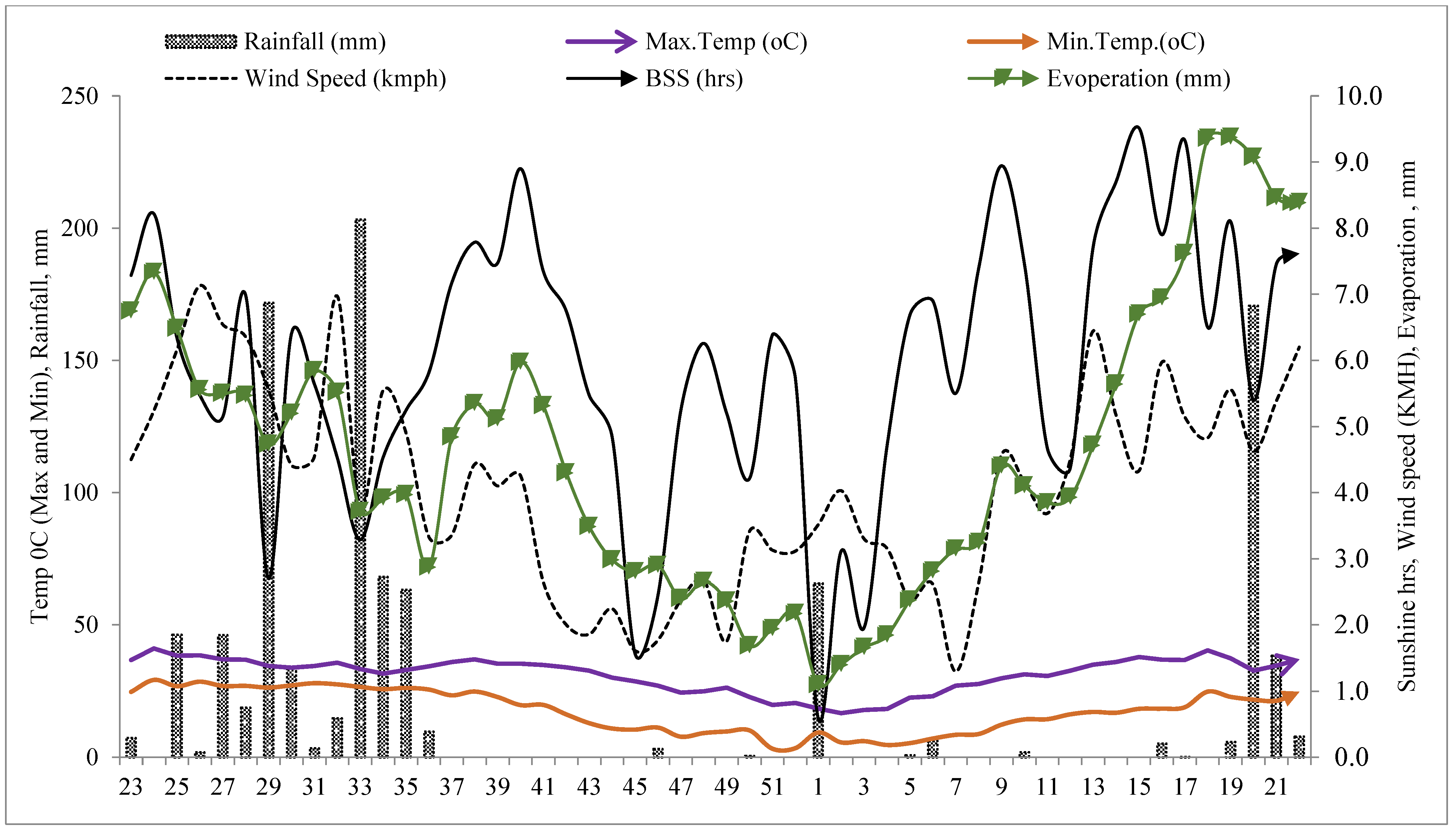
2.1. Site Description and Prevailing Weather Conditions

During 2020–2021 and 2021–2022, ten IFS modules were evaluated in a one-acre area of the experimental field at the Indian Council of Agriculture Research (ICAR)–Indian Agricultural Research Institute (IARI), New Delhi. It is located at 28°38′ N latitude, 77°10′ E longitude, and 228.6 m above mean sea level. The site comes under the Trans-Gangetic plains (TGP) with a sub-tropical, semi-arid climate with the characteristics of a hot, dry summer and cold winter. It was under intensive cultivation with a greater number of crops and other farm activities; hence, it is characterized as an intensive agro-ecological site. The detailed meteorological data for the study periods (2020–2021 and 2021–2022) were collected at the ICAR–IARI meteorological observatory in New Delhi, and the weather data are presented in Figure 1. During this study, the mean maximum temperatures for the years were 31.4 °C and 31.2 °C, respectively. Whereas, the mean minimum temperatures were 17.5 °C and 18.2 °C, respectively. The annual mean relative humidity was 81.5 and 84.1%, respectively. The total rainfall for the two years was 992 mm and 1749 mm, respectively. The total rainfall for the rainy season was 693.3 and 1365.6 mm, respectively, for the years 2021–2021 and 2021–2022. The mean sunshine hours and mean evaporation have been depicted in Figure 1. Similarly, in the winter season, the mean maximum and minimum temperatures were 25.3 °C and 24.6 °C, and 9.8 °C and 11.1 °C, in 2020–2021 and 2021–2022, respectively.

2.2. Soil Characteristics

The soils of the IARI New Delhi farm belong to the Mehrauli series, Inceptisol order. Before the commencement of this research experiment, composite soil samples were collected and analyzed from 0–15 cm of soil depth for the analysis of soil mechanical and chemical properties. The soil texture was sandy clay loam with a pH value of 7.7, and it was low in organic carbon (0.42%), available nitrogen (253.6 kg/ha) and available phosphorous (11.6 kg/ha), and medium in available potassium (256.2 kg/ha). The soil mechanical analysis (Hydrometer method) [19] showed a sandy clay loam texture of the soil with sand, silt, and clay proportions of 46.2, 35.6, and 18.2%, respectively.

2.3. Treatment Details

An area of 1 acre (4046.86 square meter) was undertaken to study the effect of diverse modules on productivity, profitability, livelihood, and environmental footprints. The treatments M1- RWCS, M2- MWCS, M3- AHS, M4- VP, M5- VP + PVC, M6- VP + PVC + FC, M7- VP + PVC + FC + AHS, M8- VP + PVC + FC + AHS + M, M9- VP + PVC + FC + AHS + M + BK, M10- VP + PVC + FC + AHS + M + BK + VC were studied under an integrated farming system (

Table 1. Treatment details and components of various modules of the integrated farming system.

	Treatments	Field Crops	Agri–Horti System	Open Field Vegetable Production	Protected Vegetable Production	Mushroom Production	Beekeeping	Vermicomposting
M1	RWCS	✔
M2	MWCS	✔
M3	AHS		0✔
M4	VP			✔
M5	VP + PVC			✔	✔
M6	VP + PVC + FC	✔		✔	✔
M7	VP + PVC + FC + AHS	✔	✔	✔	✔
M8	VP + PVC + FC + AHS + M	✔	✔	✔	✔	✔
M9	VP + PVC + FC + AHS + M + BK	✔	✔	✔	✔	✔	✔
M10	VP + PVC + FC + AHS + M + BK + VC	✔	✔	✔	✔	✔	✔	✔

Note: RWS: rice wheat system, MWS: maize wheat system, AHS: agri–horti system, VP: open field vegetable cultivation, PVC: protected vegetable cultivation, FC: field crops, M: mushroom production, BK: beekeeping, VC: vermicomposting. ✔ Symbol indicates inclusion of activity in IFS as mentioned above.

). Under the IFS cropping systems (CS), agri–horti systems (AHS), protected vegetable cultivation (PVC), and open field vegetable production (VP) were evaluated in a system mode for their agronomic efficacy. Further, the cropping systems, viz., baby corn–mustard–baby corn, maize–onion, okra–cabbage + broccoli + cauliflower–cowpea, bottle gourd-early vegetable pea-late wheat, cowpea–marigold–vegetable mustard, agri–horti system (AHS), protected vegetable cultivation (PVC), mushroom production, and beekeeping were experimented for and compared with existing RWS and MWS. The vermicomposting in 50 m² also integrated M10 with other components such as VP, PVC, FC, AHS, M, and BK. The detail of the treatments of various modules of IFS and area allocation have been provided in Table 1 and

Table 2. Area allocation (m²) for different modules on a hectare basis of the integrated farming system model.

	Treatments/Modules	Field Crops	Open Field Vegetable Production	Protected Vegetable Production	Agri–Horti System	Mushroom Production	Beekeeping	Vermicomposting	Total Area
M1	RWCS	10,000	-	-	-	-	-	-	10,000
M2	MWCS	10,000	-	-	-	-	-	-	10,000
M3	AHS	-	-	-	10,000	-	-	-	10,000
M4	VP	-	10,000	-	-	-	-	-	10,000
M5	VP + PVC	-	7778	2222	-	-	-	-	10,000
M6	VP + PVC + FC	1667	6111	2222	-	-	-	-	10,000
M7	VP + PVC + FC + AHS	1154	4231	1538	3077	-	-	-	10,000
M8	VP + PVC + FC + AHS + MP	1139	4177	1519	3038	127	-	-	10,000
M9	VP + PVC + FC + AHS + MP + BK	1139	4177	1519	3038	127	*	-	10,000
M10	VP + PVC + FC + AHS + MP + BK + VC	1125	4125	1500	3000	125	*	125	10,000

Note: RWS: rice wheat system, MWS: maize wheat system, AHS: agri–horti system, VP: open field vegetable cultivation, PVC: protected vegetable cultivation, FC: field crops, M: mushroom production, BK: beekeeping, VC: vermicomposting. * indicate inclusion of bee keeping as a component in IFS module without specific area allocation

.

2.4. Enterprise Management

The management of component crops in a cropping systems mode and other allied activities were done as per the standard recommended practices (Table 1, Table 2 and

Table 3. Crops, varieties, spacing, and fertilizer schedule adopted for cropping systems trial.

S N.	Crop	Crop Growing Period	Variety	Spacing (cm)	Seed Rate (kg/ha)	Fertilizer Schedule (N, P2O5 & K2O kg/ha)
1.	baby corn–mustard–baby corn
	babycorn	July–October	G-5414	45 × 15	25	120:60:60
	mustard	November–March	PM-28	50 × 10	5	60:60:40
	babycorn	March–June	G-5414	45 × 15	25	120:60:60
2.	maize–Onion
	maize	June–October	PMH-1	60 × 15	20	120:60:40
	onion	November–March	Pusa Riddhi	45 × 20	08	100:40:60
3.	okra–cabbage + broccoli + cauliflower–cowpea
	okra	June–October	Pusa A-4	50 × 50	15	100:50:60
	cabbage + broccoli + cauliflower	November–February	Pusa Ageti, Pusa Aghani, Pusa Broccoli KTS 1	45 × 30	0.5	120:60:60
				45 × 30	0.5	120:60:60
				45 × 30	0.5	120:60:60
	cowpea	June–September	Pusa Sukomal	45 × 10	25	20:60:40
4.	bottle gourd-early vegetable pea-late wheat
	bottle gourd	May–September	Amrit F1-Hybrid	250 × 100	5	200:100:100
	Early Vegetable pea	October–December	Pusa Pragati	40 × 10	75	20:60:40
	Late Wheat	December–April	HD3271	20 × 8	125	100:50:40
5.	cowpea–marigold–vegetable rapeseed
	cowpea	June–September	Pusa Sukomal	45 × 10	25	20:60:40
	marigold	October–February	Pusa Narangi Pusa Basanti	30 × 30	0.75	90:90:75
	Vegetable rapeseed	April–May	Pusa Sag-1	30 × 5	7–8	30:30:40
6	rice–wheat
	rice	July–November	Pusa Basmati 1509	20 × 10	25	90:30:30
	wheat	November–April	HD-3226	20 × 10	120	120:60:60
7	maize–wheat
	maize	June–October	PMH-1	60 × 15	20	120:60:40
	wheat	November–April	HD-3226	20 × 10	120	120:60:60

). The timely intercultural operations were done on the crops using a battery-operated mover or hand hoe depending upon the spacing of the crops. In crops such as tomatoes and okra, earthing-up was done to provide more anchorage to the seedlings. For cucurbits, the bamboo stick-based staking was provided for proper inter-cultivation and management. The field crops (maize, mustard, rice, and late-sown and timely-sown wheat) were harvested from the net plot by leaving the border rows. The dried produce was threshed mechanically and weighed after drying at appropriate storage moisture level. The marigold flowers were timely cut and weighed. The vegetables and fruit crops were also timely harvested, and the fresh weight was recorded. The baby corn harvesting was done through hand picking. An area of 1200 m² was allocated to the agri–horti system (AHS) within the IFS model. The alleys between the two rows of fruit crops were used for growing vegetables. Regular pruning of the fruit crops like phalsa, pomegranate, and karonda were done as per the requirement. Insect-pests were controlled preferably by spraying organic insecticides like neem oil, but when required, also by systemic insecticides, viz., imidacloprid. Multiplex, liquid fertilizer containing micronutrients was applied to the tree crops at 2.5 gms/L of water. For mushroom production, a room of 50 m² of an inside area was constructed near the edge of the field. For vermicomposting, four pits were dug, with the dimension of each pit measuring 3 m × 1 m × 1 m, and the total area for vermicompost component being 7.5 m × 2.5 m.

2.5. Observations Recording

2.5.1. System Equivalent Productivity

The yield obtained from individual crops in a cropping system was expressed in maize equivalent yield (1) and were added together to obtain the system equivalent productivity (2) of each cropping system. The system equivalent productivity was then expressed in maize equivalent system productivity which is calculated by combining maize equivalent yields from the summer, rainy, and winter season crops. Likewise, system production efficiency was calculated to obtain the yield produced on a daily basis (3).

$$\mathrm{Maize} \mathrm{equivalent} \mathrm{yield} (\mathrm{MEY})=\frac{\mathrm{Yield} \mathrm{of} \mathrm{a} \mathrm{crop} \times \mathrm{Market} \mathrm{value} \mathrm{of} \mathrm{the} \mathrm{crop}}{\mathrm{Market} \mathrm{value} \mathrm{of} \mathrm{maize} }$$

(1)

System maize equivalent Yield (SMEY) = Ʃ Maize equivalent yield of all crops in a cropping system

(2)

$$\mathrm{System} \mathrm{production} \mathrm{efficiency} (\mathrm{kg}/\mathrm{ha}/\mathrm{day})=\frac{\mathrm{System} \mathrm{productivity}\left(\mathrm{kg}/\mathrm{ha}\right)}{365}$$

(3)

2.5.2. System Economics

The system benefit cost ratio was calculated by dividing the system gross returns by the system cost of production (4).

$$\mathrm{System} \mathrm{benefit} \cos \mathrm{t} \mathrm{ratio} (\mathrm{B}:\mathrm{C})=\frac{\mathrm{System} \mathrm{gross} \mathrm{returns}}{\mathrm{System} \cos \mathrm{t} \mathrm{of} \mathrm{production}}$$

(4)

$$\mathrm{System} \mathrm{economic} \mathrm{efficiency} (\mathrm{USD}/\mathrm{ha}/\mathrm{day})=\frac{\mathrm{Net} \mathrm{returns} \left(\mathrm{US} \$/\mathrm{ha}\right)}{365}$$

(5)

2.5.3. Sustainable Livelihood Index

The sustainable livelihood index is a useful tool in assessing the livelihood elements of the rural poor households. The higher values of sustainability livelihood index ensure the sustainability of the enterprise [20].

$$\mathrm{Sustainability} \mathrm{livelihood} \mathrm{index}=\frac{\mathrm{Net} \mathrm{returns}-\mathrm{Standard} \mathrm{deviation}}{\mathrm{Maximum} \mathrm{net} \mathrm{returns} \mathrm{attained} \mathrm{in} \mathrm{any} \mathrm{module}}$$

(6)

2.5.4. Energetics under Different Crops/IFS Based System

Energy input and output: The total energy input of the system is calculated by summing all the energy equivalents of the inputs used in the system and is expressed in MJ/ha. Similarly, the total grain and straw yield of all the commodities of the components was first converted into a maize equivalent yield and later in terms of energy (MJ/ha) using respective energy coefficients. The total energy output is calculated by summing the energy equivalents of the grain and straw yields [21].

Net energy (MJ/ha) = Output energy (MJ/ha) – Input energy (MJ/ha)

(7)

$$\mathrm{Energy} \mathrm{productivity} (\mathrm{kg}/\mathrm{MJ})=\frac{\mathrm{MEY}(\mathrm{kg}/\mathrm{ha})}{\mathrm{Input} \mathrm{energy} (\mathrm{MJ}/\mathrm{ha})}$$

(8)

$$\mathrm{Energy} \mathrm{profitability}=\frac{\mathrm{Net} \mathrm{energy} \mathrm{gain} (\mathrm{MJ}/\mathrm{ha})}{\mathrm{Input} \mathrm{energy} (\mathrm{MJ}/\mathrm{ha})}$$

(9)

$$\mathrm{Energy} \mathrm{intensity} (\mathrm{MJ}/\mathrm{USD})=\frac{\mathrm{Output} \mathrm{energy} (\mathrm{MJ}/\mathrm{ha})}{\mathrm{Cos}\mathrm{t} \mathrm{of} \mathrm{cultivation} (\mathrm{US}\$/\mathrm{ha})}$$

(10)

2.5.5. Total Water-Use: Crops vis-à-vis Other Enterprises

The amount of water used by each crop in the cropping system is added to obtain the total water usage in the cropping system. Similarly, the total water usage by the different modules was calculated by adding the water use by each module of the IFS model and expressed in m³. The maize equivalent yield of each system is divided by the total water use from each component to obtain water productivity of the system and is expressed in kg/m³.

2.5.6. Global Warming Potential (GWP)

Greenhouse gas (GHG) emission from crop production in each cropping system and various modules was estimated using different coefficients [22]. The GHG (CO₂, N₂O, and CH₄) emitted during the crop growth cycle was estimated and expressed in a CO₂ equivalent [23].

The CH₄ emission from submerged rice fields and N₂O emissions from upland crops and crop residue were calculated by the given formula [24]:

CH₄ emission (kg year⁻¹) = EF × SF₀ × (Aj + [Aj × SFj])/10

(11)

where, EF = 10 g m⁻² year⁻¹ for India; Aj = area under rice paddy, ha year⁻¹; SF₀ = 1.4 correction factor for organic amendments; SFj = 0.7 scaling factor for A.

Likewise, to quantify N₂O emissions, the 0.01 emission factor was multiplied by the total N employed through various organic sources and expressed in N₂O kg N input⁻¹ [25].

$${\mathrm{N}}_2\mathrm{O} \mathrm{emission}\left({\frac{\mathrm{kg}}{\mathrm{yr}}}^{ }\right)=\mathrm{N} \mathrm{contributed} \mathrm{by} \mathrm{N} \mathrm{sources} \times 0.01\times 44/28$$

(12)

Total global warming potential (GWP) from rice and other upland crops was estimated as:

Total GWP from crops = ∑ CF₁ ith crops

(13)

and the GWP of each crop is estimated as:

$$\mathrm{GWP}={\mathrm{Total} \mathrm{N}}_2\mathrm{O} \mathrm{emission} \times 265+{\mathrm{Total} \mathrm{CO}}_2 \mathrm{emission}$$

(14)

The CO₂-eq was obtained by multiplying the GWP equivalent of 28, 1, and 265 for CH₄, CO₂, and N₂O, respectively, for a 100-year timeframe [26]. The GHG emitted from carrying out the farm operations (land preparation, pest protection, weed management, fertilizer application, irrigation, and harvesting) and production of seeds were multiplied with the respective emission coefficient [24]. Likewise, greenhouse gas intensity (GHGI) is the ratio of the global warming potential to the maize grain equivalent yield and it is expressed as kg CO₂ e/kg MEY [24].

3. Results

3.1. Agronomic Productivity of Cropping System Module

A significant variation in the agronomic productivity and system maize equivalent yield (SMEY) of the seven cropping systems was observed (

Table 4. Agronomic productivity (kg/ha), equivalent yields (kg/ha), and production efficiency (kg/ha/day) of different cropping systems under integrated farming systems.

Cropping System	Agronomic Productivity of Crops			Maize Equivalent Yield			SMEP	PE
	Rainy Season	Winter	Summer	Rainy Season	Winter	Summer
Rice–wheat	4356	4867	-	8189	5222	-	13,411	36.7
Maize–wheat	5844	5289	-	5844	5678	-	11,522	31.6
baby corn–mustard–baby corn	7100	1567	7478	7633	4089	8044	19,767	54.2
Maize–onion	5900	14,856	-	5900	23,944	0	29,844	81.8
Okra–cabbage + brocali + cauliflower–cowpea	8156	16,011	7856	11,978	17,211	8456	37,644	103.1
Bottle gourd–pea-–wheat	13,611	8189	3278	14,622	13,211	3522	31,356	85.9
Cowpea–marigold–veg mustard	7967	9167	13,150	8567	14,783	14,133	37,483	102.7
SEm±	-	-	-	-	-	-	1813	4.93
LSD (p = 0.05)	-	-	-	-	-	-	5650	15.4

Note: SMEP: system maize equivalent productivity, PE: production efficiency.

). The highest agronomic productivity (13,611, 14,856, and 13,150 kg/ha) and MEY (14,622, 23,944, and 14,113 kg/ha) was obtained in bottle gourd, onion, and vegetable mustard during the rainy, winter, and summer seasons, respectively. The highest SMEY was, however, recorded in okra–cabbage + broccoli + cauliflower–cowpea cropping system (37,644 kg/ha) which remained on a par with the cowpea–marigold–vegetable mustard cropping system (37,483 kg/ha). The minimum SMEY was recorded in MWS, followed by RWS (11,522 and 13,411 kg/ha, respectively). A 180.6 and 226.7% increase in the SMEY was obtained in the okra–cabbage + broccoli + cauliflower–cowpea cropping system over RWS and MWS, respectively. The seasonal increase in MEY under the okra–cabbage + broccoli + cauliflower–cowpea cropping system was 39.6 and 87.2% during the rainy and winter seasons over RWS. This varied with the 105 and 203% under the okra–cabbage + broccoli + cauliflower–cowpea cropping system over MWS. The production efficiency of the seven cropping systems followed a similar trend as SMEY (Table 4). The higher production efficiency was recorded in the okra–cole crops–cowpea cropping system with 103.1 kg/ha/day, and the production efficiency of cowpea–marigold–vegetable mustard (102.7 kg/ha/day) remained on a par with it. The minimum production efficiency was recorded in MWS (31.6 kg/ha), followed by RWS (36.7 kg/ha/day). The production efficiency declined by 180.1 and 183.4% in RWS over the okra–cole crops–cowpea cropping system.

3.2. Economics, Employment and Livelihood of Cropping Systems

The economics of seven cropping systems showed that the highest net returns (NR) (6789 USD/ha), B:C (4.33), and system profitability (18.59 USD/ha/day) were obtained in the cowpea–marigold–vegetable mustard cropping system, okra–cole crops–cowpea, being on a par with it in terms of NR (6325.8 USD/ha) and system profitability (17.33 USD/ha/day). The cereal-based systems, both RWS and MWS, recorded minimum NR (1451 USD/ha and 1147.2/ha) and B:C (1.85 and 1.73), respectively (

Table 5. System net returns, benefit cost ratio, profitability, system livelihood index (%), and employment generation (man-days) of cropping system modules.

Cropping System.	SNR (USD/ha)	B:C	System Profitability (USD/ha/day)	System Livelihood Index	Employment Generation
Rice–wheat	1451	1.85	3.97	−13.6	187
Maize–wheat	1147	1.73	3.14	−21.1	162
Baby corn–mustard–baby corn	2519	2.18	6.90	13.0	141
Maize–onion	4963	3.4	13.59	73.7	218
Okra–cole crops–cowpea	6326	3.49	17.33	107.5	282
Bottle gourd–early pea-wheat	4983	3.07	13.65	74.2	194
Cowpea–marigold–veg mustard	6789	4.33	18.59	119.0	140
SEm (±)	299.7	0.197	0.82	-	11.9
LSD (p = 0.05)	933.6	0.614	2.56	-	37.0

Note: SMEP: system maize equivalent productivity, PE: production efficiency.

). The baby corn–mustard–baby corn system recorded a 74% increase in NR over RWS and MWS. The other cropping systems, with the inclusion of vegetables, recorded a significantly higher NR, up to 368 and 492% over RWS and MWS, respectively. The difference in the system profitability was found to be non-significant under the cowpea–marigold–vegetable mustard and okra–cabbage + broccoli + cauliflower–cowpea systems, respectively. The predominant cropping systems among the marginal land holders in IGP zones, i.e., RWS and MWS, recorded the minimum system profitability (1.85 and 1.73 USD/ha/day). The baby corn–mustard–baby corn system also estimated lower system profitability (6.90 USD/ha/day) over the remaining vegetable-based systems, where the system profitability was recorded with more than 10 USD/ha/day.

The sustainable livelihood index (SLI) of different cropping systems varied significantly among different treatments (Table 5). The highest SLI (119%) was recorded in the cowpea–marigold–vegetable mustard system, followed by the okra–cole crops–cowpea system (107.5%). The SLI under RWS and MWS remained negative (−13.6 and −21.1%, respectively) as compared to vegetable-based systems. Among the two cereal-based systems, MWS has been found to be more sustainable over RWC. The employment generation opportunities were found to be higher in vegetable-based systems (Table 5). The highest employment generation was recorded from the okra–cole crops–cowpea system with an engagement of 282 man-days/year, followed by the maize–onion system (218 man-days). The minimum employment generation was observed in the baby corn–mustard–baby corn system (141 man-days/year) and the cowpea–marigold–vegetable mustard system (140 man-days/year). A higher total of 95 and 120 man-days/year were employed under the okra–cole crops–cowpea system over RWS and MWS, respectively.

3.3. Agri-Horti System Module: Agronomic Productivity and Production Efficiency

In the agri–horti system (AHS), the vegetable crops were intercropped in the alleys of the fruit trees as an income-generating component of IFS. The SMEY and the production efficiency indicates a wide variability among different AHS (

Table 6. System maize equivalent yield (kg/ha) and production efficiency (kg/ha/day) of the agri–horti system.

Vegetables under Agri-Horti System	Fruit	2020–2021	2021–2022	SMEY (Pooled)	PE
Okra–Cauliflower–Vegetable Cowpea	Guava	31,500	31,590	31,544	86.4
Spinach–Garlic–Lettuce	Pomegranate	46,740	46,550	46,644	127.8
Sponge gourd–Radish–Lettuce	Pomegranate	56,390	52,620	54,504	149.3
Coriander–Vegetable Mustard–Tomato	Guava	43,500	44,410	43,954	120.4
Spinach–Cauliflower–Coriander	Kinnow	42,940	48,730	45,834	125.6
Chilli–Brinjal	Karonda	30,110	33,800	31,951	87.5
Bitter gourd–Potato	Aonla	23,010	21,050	25,027	60.3
Safflower–Fenugreek	Phalsa	6800	8170	7485	20.5
Onion–Fenugreek	Phalsa	25,950	24,810	23,380	69.5
SEm±		2280	2210	2300	6.2
LSD (p = 0.05)		6890	7020	6953	18.8

Note: SMEP: system maize equivalent productivity, PE: production efficiency.

). Within different fruit crops, the highest SMEY was recorded under pomegranate-based AHS. Among different vegetable-based systems, sponge gourd–radish–lettuce (54,504 kg/ha) resulted in the highest economic yield, followed by the spinach–garlic–lettuce yield (46,644 kg/ha), both grown in the alleys of pomegranate-based AHS. Likewise, a significantly higher production efficiency was observed under pomegranate-based AHS, with sponge gourd–reddish–lettuce (149.3 kg/ha/day) and spinach–garlic–lettuce systems (127.8 kg/ha/day). It was followed by the guava- and kinnow-based AHS which recorded higher system production efficiency, 125.6 and 120.4 kg/ha/day, respectively. Here, the lowest SMEY was recorded in phalsa-based AHS with safflower–fenugreek (7485 kg/ha).

3.4. Productivity, Economics, Livelihood, and Employment Generation of IFS Modules

System maize equivalent productivity (SMEP) of all the ten modules under the IFS model was observed, and it varied significantly among them (

Table 7. System maize equivalent productivity (kg/ha), economics, sustainable livelihood index (%), and employment generation (man-days) of different modules of the integrated farming system.

Symbol	IFS Modules	System Maize Eqvalent Yield	Gross Returns (USD/ha)	Cost of Cultivation, USD/ha	Net Returns (USD/ha)	B:C	Profitability (USD/ha/day)	Sustainable Livelihood Index	Employment Generation
M1	RWCS	13,417	3159	1824	1335	1.73	3.7	−15.6	187
M2	MWCS	11,518	2712	1673	1038	1.62	2.8	−18.8	162
M3	AHS	34,192	8050	2592	5458	3.11	14.9	28	477
M4	VP	27,722	6528	1840	4688	3.55	12.8	19.9	468
M5	VP + PVC	54,534	12,838	6179	6658	2.08	18.2	40.7	620
M6	VP + PVC + FC	56,786	13,368	6488	6880	2.06	18.8	43.1	690
M7	VP + PVC + FC + AHS	49,840	11,733	5503	6231	2.13	17.1	36.2	625
M8	VP + PVC + FC + AHS + MP	73,925	17,405	8496	8908	2.05	24.4	64.5	756
M9	VP + PVC + FC + AHS + MP + BK	74,871	17,627	8620	9007	2.04	24.7	65.6	773
M10	VP + PVC + FC + AHS + MP + BK + VC	83,062	18,268	8822	9446	2.07	25.9	70.2	792
	SEm (±)	3230	745	0	394	0.14	1.1	-	35.5
	LSD (p = 0.05)	9671	2230	0	1179	0.42	3.2	-	106.2

Note: RWS: rice wheat system, MWS: maize wheat system, AHS: agri–horti system, VP: open field vegetable cultivation, PVC: protected vegetable cultivation, FC: field crops, M: mushroom production, BK: beekeeping, VC: vermicomposting.

). The highest SMEP was recorded from the M₁₀ module (83,062 kg/ha) which remained on a par with the M₉ (74,871 kg/ha) and M₈ (73,925 kg/ha) modules. A significantly lower SMEP was observed in MWS (11,518 kg/ha) and RWS (13,417 kg/ha). The gross income of the IFS modules significantly varied depending on the level and degree of integration of the enterprises (Table 7). The inclusion of different enterprises in the system significantly increased the gross income of the farm. A higher gross income was recorded in the M₁₀ module (18,268 USD/ha); however, it remained statistically on a par with the M₉ (17,627 USD/ha) and M₈ (17,405 USD/ha) modules. Lower gross returns were obtained from the cereal-centric systems, viz., RWS and MWS (3159 and 2712 USD/ha, respectively). Similarly, a higher net income was obtained from more diversified systems with a greater number of enterprises integrated together (M₁₀, M₉, and M₈) as compared to less diversified systems such as RWS and MWS. The highest net returns (9446 USD/ha) were obtained in M₁₀, and significantly lower net returns were obtained in MWS (1038 USD/ha) and RWS (1335 USD/ha). An almost 7- and 9-folds increase in net returns was observed by diversifying the agricultural components from RWS and MWS, respectively.

The benefit cost ratio (B:C) was also observed to be highest in the vegetable-based farming system modules as compared to the others. The highest B:C was obtained under the M₄ module (3.55) with sole vegetable cultivation followed by AHS (fruit tree and vegetable components), over other IFS modules, probably due to its higher market price and demand around the year. The B:C for other IFS-based modules remained in the range of 2.04 to 2.13 and were higher over the B:C obtained in RWS (1.73) and MWS (1.62). The diversified farming system also increased the system profitability significantly. A higher system profitability was recorded from the M₁₀ module (25.9 USD/ha/day), which remained on a par with the M₉ (24.7 USD/ha/day) and M₈ (24.4 USD/ha/day) modules. Under cereal-based systems, viz., RWS and MWS, a system profitability of 3.7 and 2.8 USD/ha/day was obtained, respectively. The higher SLI were recorded from the M₁₀ module (70.2%) followed by the M₉ module (65.6%) and the M₈ module (64.5%). Under RWS and MWS, a negative SLI (−15.6 and −18.8) was recorded due to poor net returns and higher standard deviation from other modules. The highest number of man-days/year was employed in the M₁₀ module (792 man-days/year), which was found to be statistically on a par with the M₉ (773 man-days/year) and M₈ modules (756 man-days/year). However, the minimum number of employment generation opportunities was recorded in MWCS and RWCS (162 and 187 man-days, respectively).

3.5. Energetics under IFS Model

A significant deviation in energy usages and energy productivity was observed among different modules and their integration under the IFS model (

Table 8. Energy output, input and net energy (MJ/ha), energy productivity (kg/MJ), intensity (MJ/₹) and profitability under diverse modules of the integrated farming system.

Symbol	IFS Modules	Energy Input (×103 MJ/ha)	Energy Output (×103 MJ/ha)	Net Energy (×103 MJ/ha)	Energy Productivity (kg/MJ)	Energy Intensity (MJ/US$)	Energy Profit
M1	RWCS	38.8	333.2	294.4	0.35	182.7	7.58
M2	MWCS	36.5	369.4	332.8	0.32	220.8	9.11
M3	AHS	37.2	192.6	155.4	0.92	74.3	4.18
M4	VP	36.4	447.2	410.8	0.76	190.9	11.29
M5	VP + PVC	40.0	520.9	480.9	1.36	72.2	12.03
M6	VP + PVC + FC	41.0	521.8	480.8	1.39	80.4	11.73
M7	VP + PVC + FC + AHS	39.8	420.5	380.6	1.25	76.4	9.56
M8	VP + PVC + FC + AHS + MP	54.0	420.8	366.7	1.37	49.5	6.78
M9	VP + PVC + FC + AHS + MP + BK	54.6	421.2	366.6	1.37	48.9	6.71
M10	VP + PVC + FC + AHS + MP + BK + VC	55.2	416.8	361.5	1.50	47.2	6.54
	SEm (±)	2.5	23.5	21.1	0.07	5.21	0.55
	LSD (p = 0.05)	7.5	70.4	63.1	0.22	11.5	1.65

Note: RWS: rice wheat system, MWS: maize wheat system, AHS: agri–horti system, VP: open field vegetable cultivation, PVC: protected vegetable cultivation, FC: field crops, M: mushroom production, BK: beekeeping, VC: vermicomposting.

). The energy input of all ten IFS modules significantly varied depending on the type of integration with the enterprises. The highest energy input of 55.2 × 10³ MJ/ha was incurred in the M₁₀ module due to the integration of a maximum number of diverse enterprises. It was followed by the M₉ (54.6 × 10³ MJ/ha) and M₈ modules (54 × 10³ MJ/ha). A low energy input was recorded in AHS (37.2 × 10³ MJ/ha), and the minimum input was recorded in open field vegetable cultivation (36.4 × 10³ MJ/ha). The higher energy output incurred in the M₆ module, where open field vegetable production was integrated with the protected vegetable cultivation and field crops (521.8 × 10³ MJ/ha). It was followed by the M₅ module, where open field vegetable production was integrated with the protected vegetable cultivation (520.9 × 10³ MJ/ha). A lower energy output was recorded in the M₃ module (192.6 × 10³ MJ/ha). The highest net energy was recorded in the M₅ module (480.9 × 10³ MJ/ha), which remained on a par with the M₆ module (408.8 × 10³ MJ/ha). The minimum net energy was recorded in AHS (164.7 × 10³ MJ/ha). However, a higher energy productivity was recorded in the M₁₀ module (1.50 kg/MJ); M₉ and M₈ remained on a par with it. A minimum energy productivity was incurred in MWCS (0.32 kg/MJ), followed by RWS (0.35 kg/MJ). A 328.6 and 368.7% increase in the energy productivity was recorded with M₁₀ over RWS and MWS, respectively. The maximum energy intensity was recorded under MWS (220.8 MJ/USD), followed by M4 (190.9 MJ/USD). The minimum energy intensity was however recorded with M₁₀ module (47.2 MJ/USD), where integration of maximum number of enterprises was conducted. It indicates that 74.2 and 78.6% less energy intensity is being utilized in the M₁₀ module as compared to MWS. However, the maximum energy profitability was recorded in the M₅ module, where vegetable cultivation was integrated with protected vegetable cultivation for year-round production which provided a balanced food–energy trade off.

3.6. Global Warming Potential

The global warming potential (GWP) significantly varied (p ≤ 0.05) among different modules of the IFS, depending on the input needed for the production system (

Table 9. Greenhouse gas emission, water footprints, and nitrogen addition through farm wastes under diverse modules of the integrated farming system.

	IFS Modules	Green House Gas (GHGs) Emission		Water Footprint			Nitrogen Addition through Farm Wastes (kg/ha)
Symbol		GWP (kg CO2 e)	GHGI (kg CO2 e/kg MEY)	Total Water Use, m3	Water Productivity, kg/m3	Water Footprint lit/kg Produce	Crop Residues	Mushroom Spent Compost	Vermicomposting	Total
M1	RWCS	2652	0.198	17,144	0.78	1277	38.8	0	0	38.8
M2	MWCS	2907	0.252	11,799	0.98	1024	42.3	0	0	42.3
M3	AHS	4580	0.134	15,895	2.15	465	38.2	0	0	38.2
M4	VP	2375	0.086	10,018	3.08	361	31.4	0	0	31.4
M5	VP + PVC	3817	0.070	9439	6.47	173	25.6	0	0	25.6
M6	VP + PVC + FC	4385	0.077	11,018	5.16	194	56.2	0	0	56.2
M7	VP + PVC + FC + AHS	4444	0.089	12,600	3.96	253	50.9	0	0	50.9
M8	VP + PVC + FC + AHS + MP	8163	0.110	12,477	5.93	169	38.8	55.3	0	94.1
M9	VP + PVC + FC + AHS + MP + BK	8177	0.109	12,477	6.00	167	38.8	55.3	0	94.2
M10	VP + PVC + FC + AHS + MP + BK + VC	8107	0.098	12,357	6.72	149	22.6	54.6	37.7	114.9
	SEm (±)	298	0.008	746	0.29	18.0	-	-	-	4.6
	LSD (p = 0.05)	969	0.023	2231	0.85	53.9	-	-	-	13.9

Note: RWS: rice wheat system, MWS: maize wheat system, AHS: agri–horti system, VP: open field vegetable cultivation, PVC: protected vegetable cultivation, FC: field crops, M: mushroom, production BK: beekeeping, VC: vermicomposting.

). A significantly higher GWP was noticed in more diversified modules due to the diverse input demands and higher EFPs. The highest GWP was recorded in M₉ (8177 kg CO₂ e/ha), which remained statistically on a par with the M₈ (8163 kg CO₂ e/ha) and M₁₀ (8107 kg CO₂ e/ha) modules. A significantly lower GWP was recorded in the M₄ module (2375 kg CO₂ e/ha); however, it remained on a par with RWS (2652 kg CO₂ e/ha) and MWS (2907 kg CO₂ e/ha). The greenhouse gas intensity (GHGI) also varied significantly with different modules (Table 9). The cropping system-based modules, for both RWS and MWS, have a higher GHGI as compared to other diverse farming system (DFS)-based modules. The lower GHGI in DFS nullified its greater GWP effect. Therefore, they have a better GHG mitigation impact. The higher GHGI was recorded in MWCS with 0.252 kg CO₂ eq/kg MEY, followed by RWCS (0.198 CO₂ eq/kg MEY). A significantly lower GHGI was recorded in the M₅ (0.070 CO₂ eq/kg MEY) and M₆ (0.077 CO₂ eq/kg MEY) modules, respectively. The module M₁₀, where VP + PVC + FC + AHS + MP + BK were integrated, recorded the highest GWP (8177 kg/ha CO₂ e), while the minimum GHGI (0.07 kg CO₂ e/kg MEY) was recorded in the VP + PVC module.

3.7. Water Budgeting and Environmental Implications

The total water usage and water productivity of different modules under the IFS model have been presented in Table 9. The water usage remained highest in RWS (17,144 m³), followed by AHS (15,895 m³). A significantly lower water usage was recorded from the M₅ module (9439 m³). The integration of protected vegetable cultivation required lesser water due to the use of a drip method of irrigation. A higher water productivity was recorded from the M₁₀ module (6.72 kg/m³) which remained on a par with the M₅ (6.47 kg/m³), M₉ (6.0 kg/m³), and M₈ (5.93 kg/m³) modules. A significantly lower water productivity was recorded from RWS (0.78 kg/ha) and MWS (0.98 kg/ha). The water footprint (WFP) varied between 149–1277, l/kg of the farm produce. The highest WFPs was obtained in RWS (1277 l/kg of the farm produce) and MWS (1024, l/kg of the farm produce). This thus supports the notion that a suitable designed IFS module is water-use efficient under marginal landholding.

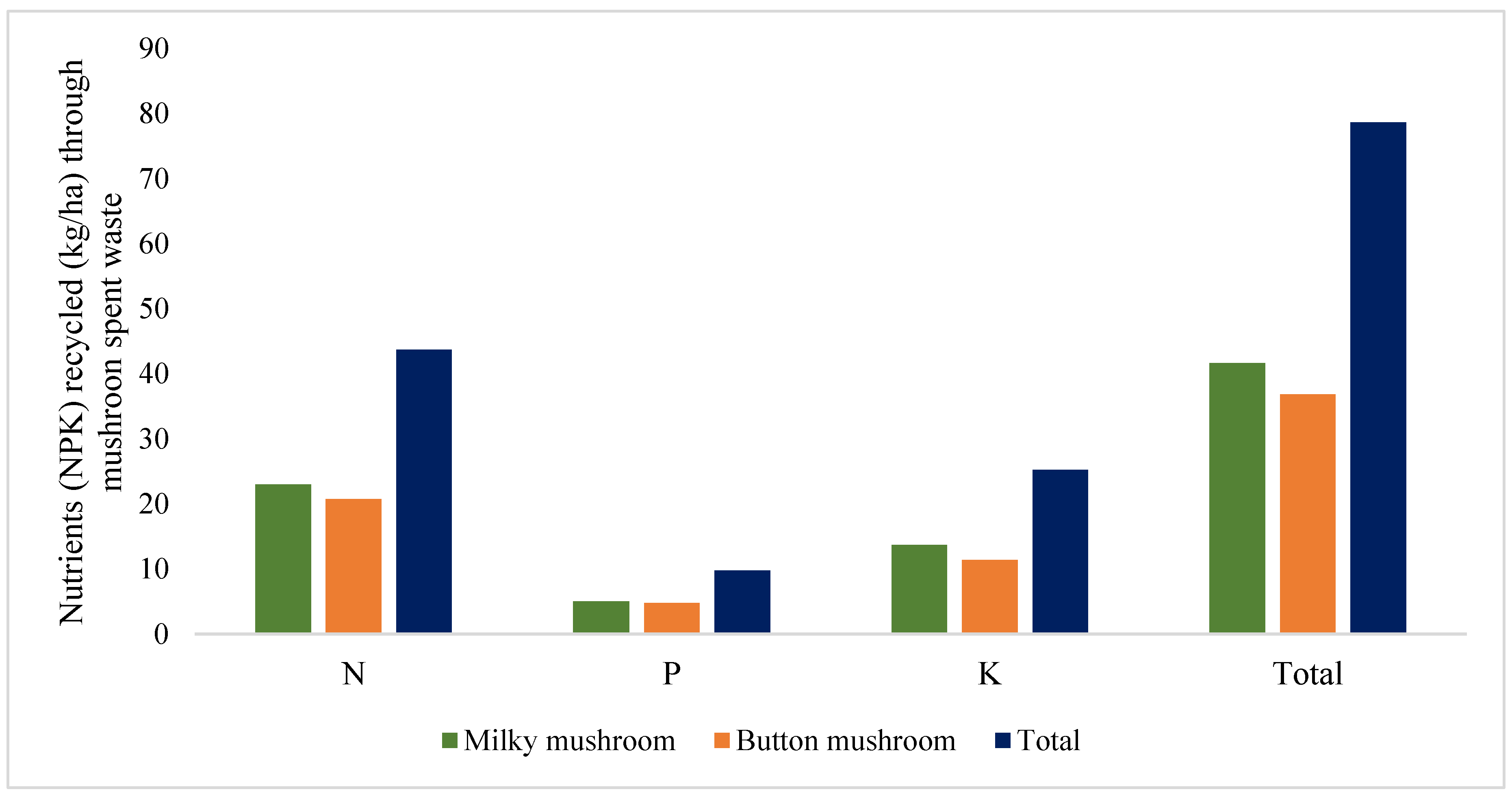
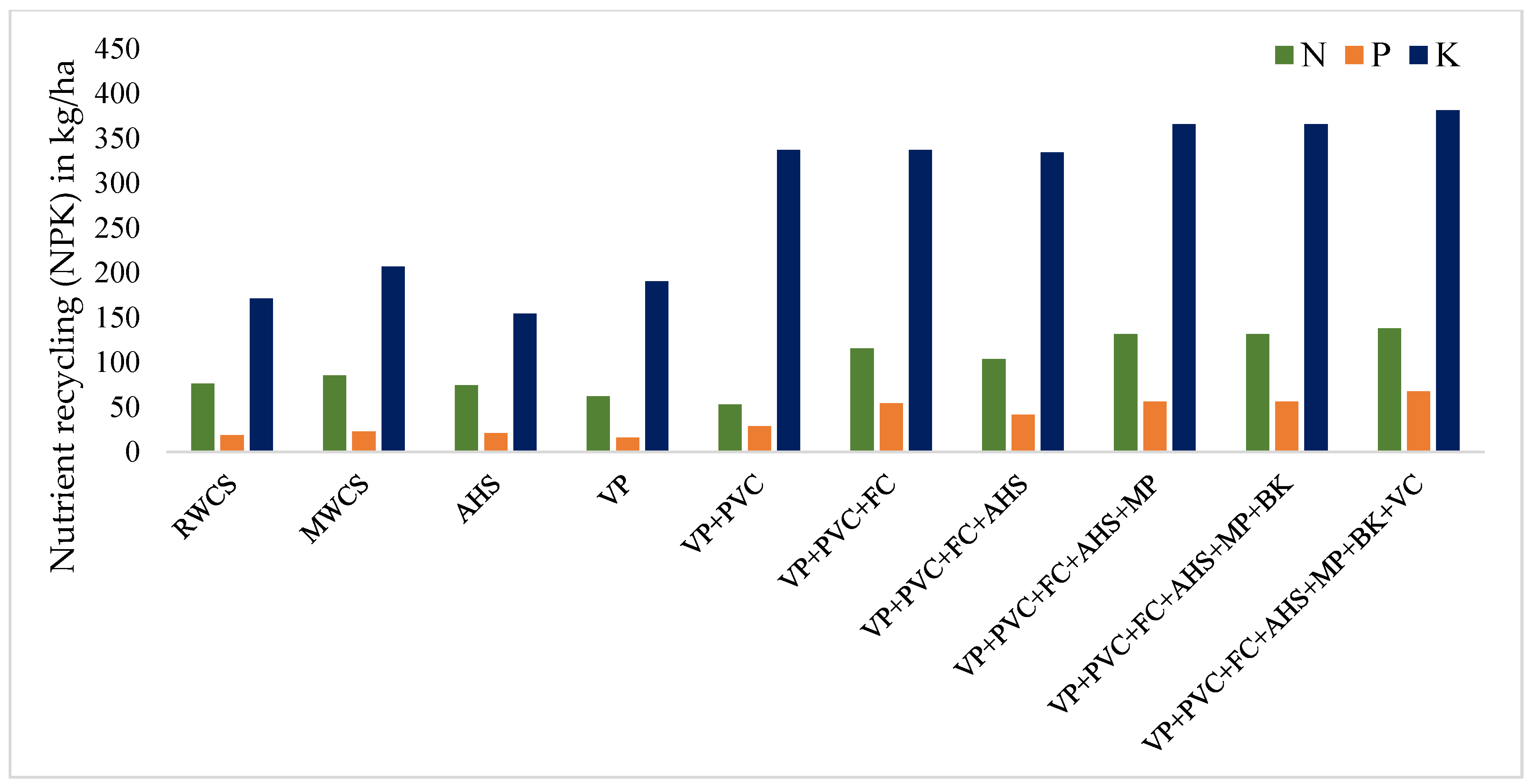
3.8. Nutrient Recycling from Different Wastes in IFS

A substantial amount of nutrients is often recycled under IFS due to diverse usages of crop and other organic wastes (Table 9 and Figure 2 and Figure 3). The maximum amount of nitrogen (N) was recycled through crop residue and across different modules (Table 9). The vegetable production-based module VP + PVC + FC and VP + PVC + FC + AHS resulted in the maximum amount of N (56.2 and 50.9 kg N/ha, respectively), while the range of N recycling from crop residue remained between 22.61 to 56.2 kg/ha. Other sources of N addition were mushroom-spent compost (Figure 2) and vermicomposting, and in the M₈, M₉, and M₁₀ modules, more than 50 kg N was recycled through mushroom-spent compost; however, M₁₀, which was integrated with the vermicompost unit, resulted in 138.2 kg recycling of N. The maximum amount of recycled nutrient nitrogen through various types of organic wastes remained highest in the M₁₀ module (114.9 kg available N/ha). The module integrating different income-generating components such as VP + PVC + FC + AHS + MP (M₈) resulted in the next-best module in recycling a higher amount of N (94 kg/ha). Module M₅ (VP + PVC) recorded the minimum amount of N recycling (25.6 kg/ha) through various means available within the module. Mushrooms contributed about 80 kg of available NPK through their spent organic waste (Figure 2). Thus, complimentary integration of diversified enterprises resulted in a higher amount of nutrient addition and recycling of scarce and expensive resources, besides adding nutritional security to meet out protein deficiency (Figure 3). The M₆ to M₁₀ modules resulted in higher addition/recycling of nutrients (NPK), and within NPK, K added the maximum quantity (Figure 3).

4. Discussion

4.1. Agronomic Productivity of Cropping System Module

The integration of different compatible enterprises in a system mode has been reported to increase productivity and economics, along with enhanced resource-use efficiency for marginal land holdings [27,28]. FAO, 2020 also reported advantages due to the adoption of IFS by small land holders [28]. IFS is an effective technological intervention for sustaining these farm typologies. The paradigm shifts in such farms through IFS technology; backstopping might enhance productivity, profitability, and environmental safety [17]. Among different cropping systems under the field crop modules of IFS, the enhanced yield from vegetable-based crop diversification over cereals-centric cropping systems was mainly due to the higher yield, regular demand, and high market price for vegetable crops as compared to cereals [29,30,31,32]. The vegetable-based crop diversification stabilizes farmers’ income, deals with climate change risks, builds up resilience and significantly improves the regular farm output [33,34]. The diversification of small farms through vegetable-based systems (okra–cabbage + broccoli + cauliflower–cowpea) resulted in higher production, ensured higher availability of diverse food, and improved economic efficiency by increasing synergy between the enterprises in resource use [35,36]. A well-designed farming system, integrating cropping systems and allied enterprises while intensifying the production system of marginal land holders, remains the key to sustain these small farms [30,31,32].

4.2. Economics, Employment and Livelihood of Cropping Systems

Diversified cropping with pulses, oilseeds, and high value crops, such as flowers, with recent technological interventions in IFS, aid in enhancing overall economics and livelihood security, besides ecological considerations [12,36,37,38]. Positive financial budgeting determines the practical acceptability of any intervention [37,38,39]. Higher production, more cycles of vegetable produce increased per unit output, profitability, and livelihood are obtained through income enhancement and poverty reduction. Higher net returns and B:C were obtained under vegetable-based systems [40] due to the frequent nutrient cycling with growing multiple vegetables. It improved soil fertility through nutrient addition and recycling. Cereal crops require intensive care and technical inputs, which may be the reasons for the escalating cost of production in RWS [41,42,43]. More than 50% enhancement in annual man-days involvement was due to year-round cultivation of the okra–cabbage + broccoli + cauliflower–cowpea system over traditional RWS [11,40]. More man-days were also engaged in this system because of staggered harvesting of the produce in cole crops and regular picking in okra and vegetable cowpea. Therefore, inclusion of vegetable crops in the model increased the system employment generation over field crops. This also decelerated the trend of shifting manpower from farm households toward non-farm sectors for better livelihood, which may supplement incomes, generate employment, and reduce poverty [44,45]. The elasticity in demand of local vegetables and comparatively shorter production cycles produce a consistent income and improve the livelihood of marginal farmers [46,47]. The year-round income from vegetable production also enables the timely purchase of inputs such as seed, fertilizer, and pesticides compared to traditional crops where income is obtained once or twice a year only [48]. The contribution of adopting crop diversification with the involvement of vegetables in sustaining agriculture and agriculture-based livelihoods in small farms of developing nations has been also reported by many researchers [49,50].

4.3. System Productivity and Production Efficiency

The agri–horti system (AHS) integrated with vegetable crops resulted in higher system productivity and production efficiency [30]. The higher system productivity of pomegranate-based AHS was probably due to the compensation of the area sacrificed by canopy coverage of trees with short duration vegetables, higher land use efficiency, and economic profitability [51]. Designing suitable AHS, which can minimize the competition between fruit trees and field crops, is crucial for high productivity through optimum nutrient cycling and erosion control [52,53]. Production efficiency was also recorded higher under pomegranate, kinnow, and guava-based AHS, as these systems encompassed a higher number of vegetables [54,55]. Under an integrated farming system, a circular economy based on profitable crop production, horticulture, liquid manure preparation, and biogas, have higher nutrient recycling. The enhanced N, P, and K addition, mainly due to better residue recycling, resulted in optimum soil health [55,56,57]. As the number of enterprises to be integrated reduces, the cost of production also reduces, but since the product output also reduces, the net returns reduced with single enterprises [57,58]. The highest B:C was obtained with M₄ (vegetable production), but the more diversified and highly profitable products such as mushroom, honey, vegetables, etc., obtained under M₁₀ provided better opportunities for livelihood security and reduced pollution due to waste management and reducing GHG emission and thereby maintaining ecosystem stability [59]. The per day profitability, SLI, and employment generation was also recorded highest under M₁₀ due to the efficient utilization of farm waste that reduces the dependence on external input use, making the enterprises self-sustainable by generating wealth from waste. The judicious integration and synergism among enterprises and efficient byproduct utilization also reduces the risk of crop failure and losses. The negative SLI (−15.6 and −18.8) in RWS and MWS was mainly due to a higher standard deviation of all the ten modules as compared to net returns from these two systems [60].

4.4. Energetics under IFS Model

Food production systems require a huge amount of energy; thus, choosing the appropriate module under an established IFS on the basis of energy auditing is very crucial in making them sustainable [32,40]. The highest energy input was incurred in the M₁₀ module due to the inclusion of multiple labor-intensive components such as mushroom cultivation, vegetable production etc., which needed a higher energy input per unit area [21,30,61,62]. The higher marketable and surplus produce and the cost of labor involved under the M₁₀ module enhanced the energy input. However, the energy output obtained its maximum under vegetable-based systems due to short life cycles and more produce per unit of area. In addition, energy profitability was higher under vegetable-based systems due to optimum inter-spatial arrangement and its utilization for higher resource conversion. The maximum net energy was in vegetable-based modules, M₅ and M₆, due to their higher energy output; however, higher economic produce per unit of energy use was the reason for enhanced energy productivity with the M₁₀ module [9,63,64,65]. Reducing the energy input and improving energy output increases the energy use efficiency which enhances farm sustainability [9,13,66]. The energy intensity remained highest in MWS, followed by vegetable production and RWS, due to higher mechanization and intensive soil cultivation, which require more energy per unit of monetary input. Thus, the economic returns under M₁₀ had a positive correlation with energy productivity but a negative correlation with GHGI and energy intensity; this confirms its effectiveness for reducing EFPs under IFS [61]. The poor net energy in RWS and MWS indicates that these systems are not energy-efficient systems and must be diversified by including the enterprises that are intricately linked and are mutually complimentary [61,65].

4.5. Global Warming Potential, Environmental Implications and Water Budgeting

The predictable mean GHG emissions were negative or neutral for IFS models in 11 agro-climatic zones (ACZs) out of the 15 ACZs [54]. Thus, cleaner production technologies such as IFS can potentially help to meet out the target of reducing GHG emissions. A significantly higher GHG mitigation impact was in diversified production systems due to the efficient use of resources [62,63]. The environmental dividends in IFS were mainly due to efficient water, energy, and nutrients usages and overall lesser GHG emissions by integrating crop diversification, agro-forestry systems, and other complementary enterprises [62,67]. Besides supporting food and nutritional security, it also reduces dependence on external inputs. Although the enterprise intensification increases GWP in M₁₀ due to higher energy consumption, the GHGI reduced in it, which validates the claim that integrating crop and allied activities has a better mitigation effect. Paramesh et al., [62] also highlighted the integration of rice with allied enterprises such as dairy, fish, and duck for sustainability, because integration enhances nutrients’ recycling and reduces dependence on external inputs and lesser EFPs [6]. Integration of crops with other compatible enterprises helps to increase ecosystem services, avoids adverse environmental impact, and sustains profitability [17,67]. The IFS also enhanced energy use efficiency over mono-cropping due to better synergistic interaction among the components [68,69,70,71,72]. The highest water usage was recorded in the RWS module due to puddling and continuous standing of water in the crop [32]. Higher water productivity in the diversified systems was due to the multiple use of available water with integration of different enterprises. The water supplied and the wastewater recycled from one enterprise is utilized by other components dependent upon it, and, therefore, the circular movement of water within different modules enhances water productivity under close-linked multi-enterprise modules from M₅ to M₁₀. [59]. Higher yields, farm profitability, energy-use efficiency, and water productivity with sustained/improved environmental quality in smallholder production systems of IGP of India and other similar agro-ecologies of South Asia with the adoption of IFS has been reported earlier also [40,73].

4.6. Nutrient Recycling from Different Wastes in IFS

The total crop/farm residue was recorded to be at the maximum with the M₁₀ module where all components were integrated and the amount gradually decreased with fewer enterprise integration. It was because the limited components could produce only a small amount of biomass to the module. Thus, efficient recycling of farm wastes met out the total nutrients’ requirement of the diverse crops grown under different modules via circular economy principles [74]. A higher NPK was added through milky mushrooms due to the rich composition of its media [75]. Mushroom cultivation requires low inputs and space with little maintenance; hence, it can be a viable option for rural unemployed youth, women, and other work-seeking farmers [60,76]. Likewise, Figure 3 indicates that the maximum available N, P, and K was recorded from M₅ to M₁₀ due to the greater amount of crop residue generated, recycled, and utilized for additional nutrient quantities in the soil. In the long run, this reduces the cost of production and increases farm sustainability. The single enterprise-based modules, M₁ to M₅, had limited crop residue generation. Therefore, the judicious selection of different enterprises would generate diverse types of crop/farm residue/waste that would reduce energy dependence, hence also GHG emissions. It also helps in maintaining the soil fertility and achieving the circular economy objectives by limiting the use of external inputs.

5. Conclusions

Diversification through IFS has ample potential to improve the livelihood of small and marginal farmers, as it ensures food security, enhances soil health, and promotes efficient natural resources use. The novel findings from this study confirmed the hypothesis that the crop yields, production efficiency, and overall farm income increased with lesser environmental footprints due to the judicious integration of different modules under the IFS model through the complementarity in resource use. The resource cycling among different enterprises results in fewer environmental footprints and promotes cleaner production technologies, especially under the areas where economic viability and sustainability of small and marginal farms are challenged. The inter-linked resource use and by-product recycling among different enterprises encompassing vegetable production, field crops, agri–horti systems, mushroom production, beekeeping and vermicomposting remained more profitable due to in-situ resource recycling, which reduces the cost of waste collection, processing, and transportation. The optimization of different modules paved the way for round-the-year employment, with lesser water and carbon footprints, eventually assisting in achieving a green economy. The present study suggests that the bio-intensification through the judicious integration of vegetable cultivation+ protected vegetable cultivation+ field crops+ agri–horti system+ mushroom production+ beekeeping+ vermicomposting modules as a part of the IFS model can ensure higher productivity and enhanced income and profitability. It ensures a green economy for marginal land holders through fewer environmental footprints. However, the modules must be optimized as per the location-specific requirement of different regions on the micro-unit-based financial budgeting.

References

1. D’amato, D.; Korhonen, J. Integrating the green economy, circular economy and bioeconomy in a strategic sustainability framework. Ecol. Econ. 2021, 188, 107143. [Google Scholar] [CrossRef]
2. Lu, Z.; Broesicke, O.A.; Chang, M.E.; Yan, J.; Xu, M.; Derrible, S.; Mihelcic, J.R.; Schwegler, B.; Crittenden, J.C. Seven approaches to manage complex coupled human and natural systems: A sustainability toolbox. Environ. Sci. Technol. 2019, 53, 9341–9351. [Google Scholar] [CrossRef] [PubMed]
3. Mihelcic, J.R.; Crittenden, J.C.; Small, M.J.; Shonnard, D.R.; Hokanson, D.R.; Zhang, Q.; Chen, H.; Sorby, S.A.; James, V.U.; Sutherland, J.W.; et al. Sustainability science and engineering: The emergence of a new Meta discipline. Environ. Sci. Technol. 2003, 37, 5314. [Google Scholar] [CrossRef] [PubMed]
4. Broman, G.I.; Robert, K.H. A framework for strategic sustainable development. J. Clean. Prod. 2017, 140, 17–31. [Google Scholar] [CrossRef]
5. Lal, R. Integrating Animal Husbandry with Crops and Trees. Front. Sustain. Food Syst. 2020, 4, 00113. [Google Scholar] [CrossRef]
6. Jurgilevich, A.; Birge, T.; Kentala-Lehtonen, J.; KaisaKorhonen-Kurki, K.; Pietikäinen, J.; Saikku, L.; Schösler, H. Transition towards Circular Economy in the Food System. Sustainability 2016, 8, 69. [Google Scholar] [CrossRef] [Green Version]
7. D’Amato, D.; Droste, N.; Allen, B.; Kettunen, M.; Lähtinen, K.; Korhonen, J.; Leskinen, P.; Matthies, B.D.; Toppinen, A. Green, circular, bio economy: A comparative analysis of sustainability avenues. J. Clean. Prod. 2017, 168, 716–734. [Google Scholar] [CrossRef]
8. Green, R.E.; Cornell, S.J.; Scharlemann, J.P.W.; Balmford, A. Farming and the fate of wild nature. Science 2005, 307, 550–555. [Google Scholar] [CrossRef] [Green Version]
9. Arizpe, N.; Giampietro, M.; Ramos-Martin, J. Food security and fossil energy dependence: An international comparison of the use of fossil energy in agriculture (1991–2003). Crit. Rev. Plant. Sci. 2011, 30, 45–63. [Google Scholar] [CrossRef]
10. Moraine, M.; Duru, M.; Therond, O. A social-ecological framework for analyzing and designing integrated crop–livestock systems from farm to territory levels. Renew. Agric. Food. Syst. 2016, 1, 43–56. [Google Scholar] [CrossRef] [Green Version]
11. Rathore, S.S.; Shekhawat, K.; Dass, A.; Premi, O.P.; Rathore, B.S.; Singh, V.K. Deficit Irrigation Scheduling and Super absorbent Polymer hydrogel Enhance Seed Yield, Water Productivity and Economics of Indian Mustard Under Semi-Arid Ecologies. Irrig. Drain. 2019, 68, 531–541. [Google Scholar] [CrossRef]
12. Rathore, S.S.; Bhatt, B.P. Productivity improvement in jhum fields through integrated farming system. Indian J. Agron. 2008, 53, 167–171. [Google Scholar]
13. Kumar, S.; Kumar, R.; Dey, A. Energy budgeting of crop-livestock-poultry integrated farming system in irrigated ecologies of eastern India. Indian J. Agric. Sci. 2019, 89, 1017–1022. [Google Scholar] [CrossRef]
14. Therond, O.; Duru, M.; Roger-Estrade, J. A new analytical framework of farming system and agriculture model diversities. A review. Agron. Sustain. Dev. 2017, 37, 21. [Google Scholar] [CrossRef]
15. Zhang, W.; Ricketts, T.H.; Kremen, C.; Carney, K.; Swinton, S.M. Ecosystem services and dis-services to agriculture. Ecol. Econ. 2007, 64, 253–260. [Google Scholar] [CrossRef] [Green Version]
16. Duru, M.; Therond, O.; Martin, G.; Martin-Clouaire, R.; Magne, M.; Justes, E.; Journet, E.P.; Aubertot, J.N.; Savary, S.; Bergez, J.E.; et al. How to implement biodiversity-based agriculture to enhance ecosystem services: A review. Agron. Sustain. Dev. 2015, 35, 1259–1281. [Google Scholar] [CrossRef]
17. Rathore, S.S.; Mishra, J.S.; Bhatt, B.P. Recommended best management practices for potential ecosystem services. Indian J. Agron. 2021, 66, 180–190. [Google Scholar]
18. Duru, M.; Therond, O.; Fares, M. Designing agroecological transitions; a review. Agron. Sustain. Dev. 2015, 35, 1237–1257. [Google Scholar] [CrossRef] [Green Version]
19. Bouyoucos, C.J. Hydrometer method improved for making particle size analysis of soil. Agron. J. 1962, 54, 464–465. [Google Scholar] [CrossRef]
20. Vittal, K.P.R.; MaruthiSankar, G.R.; Singh, H.P.; Samra, J.S. Sustainability of practices of dryland agriculture: Methodology and assessment. In All India Coordinated Research Project for Dryland Agriculture; Central Research Institute for Dryland Agriculture, Indian Council of Agricultural Research: Hyderabad, India, 2002; pp. 3–4. [Google Scholar]
21. Mittal, J.P.; Dhawan, K.C. Research Manual on Energy Requirements in Agricultural Sector; ICAR: New Delhi, India, 1998. [Google Scholar]
22. IPCC. IPCC Guidelines for National Greenhouse Gas Inventories, Prepared by the National Greenhouse Gas Inventories Programme; Eggleston, H.S., Buendia, L., Miwa, K., Ngara, T., Tanabe, K., Eds.; IGES: Hayama, Japan, 1988; pp. 20–23. [Google Scholar]
23. Lal, R. Carbon emission from farm operations. Environ. Int. 2004, 30, 981–990. [Google Scholar] [CrossRef]
24. West, T.O.; Marland, G. A synthesis of carbon sequestration carbon emissions and net carbon flux in agriculture: Comparing tillage practices in the United States. Agric. Ecosyst. Environ. 2002, 91, 217–232. [Google Scholar] [CrossRef]
25. Tubiello, F.N.; Condor-Golec, R.D.; Salvatore, M.; Piersante, A.; Federici, S.; Ferrara, A.; Rossi, S.; Flammini, A.; Cardenas, P.; Biancalani, R.; et al. Estimating Greenhouse Gas Emissions in Agriculture: A Manual to Address Data Requirements for Developing Countries; Food and Agriculture Organization of the United Nations: Rome, Italy, 2015. [Google Scholar]
26. Stocker, T.F.; Qin, D.; Plattner, G.K.; Tignor, M.; Allen, S.K.; Boschung, J.; Nauels, A.; Xia, Y.; Bex, V.; Midglev, P.M. (Eds.) Contribution of Working Group I to the Fifth Assessment Report of the Intergovernmental Panel on Climate Change. In IPCC Climate Change: The Physical Science Basis; Cambridge University Press: Cambridge, UK; New York, NY, USA, 2013; pp. 710–716. [Google Scholar]
27. FAO. The Future of Food and Agriculture—Trends and Challenges; FAO: Rome, Italy, 2017; p. 151. ISBN 978-92-5-109551-5. [Google Scholar]
28. FAO. Food and Agriculture Organization (FAO); FAO: Rome, Italy, 2022. [Google Scholar]
29. Djokoto, J.G.; Afari-Sefa, V.; Addo-Quaye, A. Vegetable diversification in cocoa-based farming systems Ghana. Agric. Food Secur. 2017, 6, 6. [Google Scholar] [CrossRef] [Green Version]
30. Rathore, S.S.; Babu, S.; Shekhawat, K.; Singh, R.; Yadav, S.K.; Singh, V.K.; Singh, C. Designing energy cum carbon-efficient environmentally clean production system for achieving green economy in agriculture. Sustain. Energy Technol. Assess. 2022, 52, 102190. [Google Scholar] [CrossRef]
31. Khanam, R.; Debarati, B.; Nayak, A.K. Crop diversification: An important way-out for doubling farmers’ income. Indian Farming 2018, 68, 31–32. [Google Scholar]
32. Singh, R.; Babu, S.; Avasthe, R.K.; Yadav, G.S. Crop Diversification and Intensification for Enhancing Livelihood Security in Sikkim; ICAR-National Organic Farming Research Institute: Gangtok, India, 2018; 36p. [Google Scholar]
33. Feliciano, D. A review on the contribution of crop diversification to Sustainable Development Goal 1 “No poverty” in different world regions. J. Sustain. Dev. 2019, 27, 795–808. [Google Scholar] [CrossRef] [Green Version]
34. Kurdyś-Kujawska, A.; Strzelecka, A.; Zawadzka, D. The Impact of Crop Diversification on the Economic Efficiency of Small Farms in Poland. Agriculture 2021, 11, 250. [Google Scholar] [CrossRef]
35. Fortes, A.R.; Ferreira, V.; Simões, E.B.; Baptista, I.; Grando, S.; Sequeira, E. Food Systems and Food Security: The Role of Small Farms and Small Food Businesses in Santiago Island, Cabo Verde. Agriculture 2020, 10, 216. [Google Scholar] [CrossRef]
36. Rivera, M.; Guarín, A.; Pinto-Correia, T.; Almaas, H.; Arnalte-Mur, L.; Burns, V.; Czekaj, M.; Ellis, R.; Galli, F.; Grivins, M. Assessing the role of small farms in regional food systems in Europe: Evidence from a comparative study. Glob. Food Secur. 2020, 26, 100417. [Google Scholar] [CrossRef]
37. He, D.-C.; Ma, Y.-L.; Li, Z.-Z.; Zhong, C.-S.; Cheng, Z.-B.; Zhan, J. Crop Rotation Enhances Agricultural Sustainability: From an Empirical Evaluation of Eco-Economic Benefits in Rice Production. Agriculture 2021, 11, 91. [Google Scholar] [CrossRef]
38. Bell, L.W.; Moore, A.D.; Kirkegaard, J.A. Evolution in crop–livestock integration systems that improve farm productivity and environmental performance in Australia. Eur. J. Agron. 2014, 57, 10–20. [Google Scholar] [CrossRef]
39. Sanderson, M.; Archer, D.; Hendrickson, J.; Kronberg, S.; Liebig, M.; Nichols, K.; Aguilar, J. Diversification and ecosystem services for conservation agriculture: Outcomes from pastures and integrated crop–livestock systems. Renew. Agric. Food Syst. 2013, 28, 129–144. [Google Scholar] [CrossRef] [Green Version]
40. Kashyap, P.; Prusty, A.K.; Panwar, A.S.; Paramesh, V.; Natesan, R.; Shamim, M.; Verma, N.; Jat, P.C.; Singh, M.P. Achieving Food and Livelihood Security and Enhancing Profitability through an Integrated Farming System Approach: A Case Study from Western Plains of Uttar Pradesh, India. Sustainability 2022, 14, 6653. [Google Scholar] [CrossRef]
41. Ravallion, M.; Datt, G. How important to India’s poor is the sectoral composition of economic growth? World Bank Econ. Rev. 1996, 10, 1–25. [Google Scholar] [CrossRef] [Green Version]
42. De Janvry, A.; Sadoulet, E. Agricultural growth and poverty reduction: Additional evidence. World Bank Res. Obs. 2010, 25, 1–20. [Google Scholar] [CrossRef] [Green Version]
43. Birthal, P.S.; Roy, D.; Negi, D.S. Assessing the impact of crop diversification on farm poverty in India. World Dev. 2015, 72, 70–92. [Google Scholar] [CrossRef]
44. Ali, M.; Abedullah, M. Economic and nutritional benefits from enhanced vegetable production and consumption in developing countries. J. Crop. Prod. 2002, 6, 145–176. [Google Scholar] [CrossRef]
45. Barghouti, S.; Kane, S.; Sorby, K.; Ali, M. Agricultural Diversification for the Poor, ARD Discussion Paper 1; The World Bank: Washington, DC, USA, 2004. [Google Scholar]
46. Joshi, P.K.; Gulati, A.; Birthal, P.S.; Tewari, L. Agricultural diversification in South Asia: Patterns, determinants and policy implications. Econ. Polit. Wkly. 2004, 39, 2457–2468. [Google Scholar]
47. Weinberger, K.; Lumpkin, T.A. Diversification into horticulture and poverty reduction: A research agenda. World Dev. 2007, 35, 1464–1480. [Google Scholar] [CrossRef]
48. Birthal, P.S.; Joshi, P.K.; Chauhan, S.; Singh, H. Can horticulture revitalize agricultural growth? Indian J. Agric. Econ. 2008, 63, 310–321. [Google Scholar]
49. Jayne, T.S.; Yamano, T.; Webber, M.; Tschirley, D.; Benfia, R.; Neven, D. Smallholder income and land distribution in Africa: Implications for poverty reduction strategies. Food Policy 2003, 28, 253–275. [Google Scholar] [CrossRef] [Green Version]
50. Bigsten, A.; Tengstam, S. Smallholder diversification and income growth in Zambia. J. Afr. Econ. 2011, 20, 781–822. [Google Scholar] [CrossRef]
51. Rathore, S.S.; Babu, S.; El-Sappah, A.H.; Shekhawat, K.; Singh, V.K.; Singh, R.K.; Upadhyay, P.K.; Singh, R. Integrated agroforestry systems improve soil carbon storage, water productivity, and economic returns in the marginal land of the semi-arid region. Saudi J. Biol. Sci. 2022, 29, 103427. [Google Scholar] [CrossRef] [PubMed]
52. Grebner, D.L.; Bettinger, P.; Jacek, P.; Siry, J.; Boston, K. Chapter 11—Common forestry practices, Editor(s): Introduction to Forestry and Natural Resources, 2nd ed.; Academic Press: Cambridge, MA, USA, 2022; pp. 265–294. ISBN 9780128190029. [Google Scholar] [CrossRef]
53. Xu, H.; Bi, H.; Gao, L.; Yun, L. Alley Cropping Increases Land Use Efficiency and Economic Profitability Across the Combination Cultivation Period. Agronomy 2019, 9, 34. [Google Scholar] [CrossRef] [Green Version]
54. Sida, T.S.; Baudron, F.; Hadgu, K.; Derero, A.; Giller, K.E. Crop vs. tree: Can agronomic management reduce trade-offs in tree-crop interactions. Agric. Ecosyst. Environ. 2018, 260, 36–46. [Google Scholar] [CrossRef]
55. Garrity, D. Agroforestry and the future of global land use. In Agroforestry-The Future of Global Land Use; Springer: Dordrecht, The Netherlands, 2012; Volume 9, pp. 21–27. [Google Scholar]
56. Wilson, M.H.; Lovell, S.T. Agroforestry—The next step in sustainable and resilient agriculture. Sustainability 2016, 8, 574. [Google Scholar] [CrossRef] [Green Version]
57. Panwar, A.S.; Prusty, A.K.; Shamim, M.; Ravisankar, N.; Ansari, M.A.; Singh, R.; Modipuram, M. Nutrient recycling in integrated farming system for climate resilience and sustainable income. Indian J. Fertil. 2021, 17, 1126–1137. [Google Scholar]
58. Birthal, P.S.; Joshi, P.K.; Roy, D.; Thorat, A. Diversification in Indian agriculture towards high-value crops: The role of smallholders. Can. J. Agric. Econ. Rev. Can. D’agroeconomie 2013, 61, 61–91. [Google Scholar] [CrossRef]
59. Singh, V.K.; Rathore, S.S.; Singh, R.K.; Upadhyay, P.K.; Shekhawat, K. Integrated farming system approach for enhanced farm productivity, climate resilience and doubling farmers’ income. Indian J. Agric. Sci. 2020, 90, 1378–1388. [Google Scholar] [CrossRef]
60. Ponnusamy, K.; Shukla, A.; Kishore, K. Studies on sustainable livelihood of farmers in horticulture-based farming systems. Indian J. Hortic. 2015, 72, 285–288. [Google Scholar] [CrossRef]
61. Morais, T.G.; Tufik, C.; Rato, A.E.; Rodrigues, N.R.; Gama, I.; Jongen, M.; Serrano, J.; Fangueiro, D.; Domingos, T.; Teixeira, R.F. Estimating soil organic carbonof sown biodiverse permanent pasturesin Portugal using near infrared spectral data and artificial neutral networks. Geoderma 2021, 404, 115387. [Google Scholar] [CrossRef]
62. Yadav, G.S.; Das, A.; Kandpal, B.; Babu, S.; Lal, R.; Datta, M.; Das, B.; Singh, R.; Singh, V.; Mohapatra, K. The food-energy-water-carbon nexus in a maize-maize- mustard cropping sequence of the Indian Himalayas: An impact of tillage-cum-live mulching. Renew. Sustain. Energy Rev. 2021, 151, 111602. [Google Scholar] [CrossRef]
63. Yrjälä, K.; Ramakrishnan, M.; Salo, E. Agricultural waste streams as a resource in the circular economy for biochar production towards carbon neutrality. Curr. Opin. Environ. Sci. Health 2022, 26, 100339. [Google Scholar] [CrossRef]
64. Paramesh, V.; Parajuli, R.; Chakurkar, E.B.; Sreekanth, G.B.; Kumar, H.C.; Gokuldas, P.P.; Mahajan, G.R.; Manohara, K.K.; Viswanatha, R.K.; Ravisankar, N. Sustainability, energy budgeting, and life cycle assessment of crop-dairy-fish-poultry mixed farming system for coastal lowlands under humid tropic condition of India. Energy 2019, 188, 116101. [Google Scholar] [CrossRef]
65. Sulc, R.M.; Franzluebbers, A.J. Exploring integrated crop—Livestock systems in different ecoregions of the United States. Eur. J. Agron. 2014, 57, 21–30. [Google Scholar] [CrossRef]
66. Martinho, V.J.P.D. Energy consumption across European Union farms: Efficiency in terms of farming output and utilized agricultural area. Energy 2016, 103, 543–556. [Google Scholar] [CrossRef]
67. Amiri, Z.; Asgharipour, M.R.; Campbell, D.E.; Armin, M. A sustainability analysis of two rapeseed farming ecosystems in Khorramabad, Iran, based on energy and economic analyses. J. Clean. Prod. 2019, 226, 1051–1066. [Google Scholar] [CrossRef]
68. Rahman, S.; Barmon, B.K. Energy productivity and efficiency of the ‘gher’ (prawn-fish-rice) farming system in Bangladesh. Energy 2012, 43, 293–300. [Google Scholar] [CrossRef] [Green Version]
69. Chand, R.; Joshi, P.; Khadka, S. Indian Agriculture Towards 2030: Pathways for Enhancing Farmers’ Income, Nutritional Security and Sustainable Food and Farm Systems. In India Studies in Business and Economics; Food and Agriculture Organization of the United Nations: Rome, Italy, 2022; p. 197. ISBN 978-981-19-0762-3. [Google Scholar] [CrossRef]
70. Wezel, A.; Casagrande, M.; Celette, F.; Vian, J.-F.; Ferrer, A.; Peigné, J. Agroecological practices for sustainable agriculture. A review. Agron. Sustain. Dev. 2014, 34, 1–20. [Google Scholar] [CrossRef] [Green Version]
71. Altieri, M.A.; Funes-Monzote, F.R.; Petersen, P. Agroecologically efficient agricultural systems for smallholder farmers: Contributions to food sovereignty. Agron. Sustain. Dev. 2012, 32, 1–13. [Google Scholar] [CrossRef] [Green Version]
72. Behera, U.K.; France, J. Integrated farming systems and the livelihood security of small and marginal farmers in India and other developing countries. In Advances in Agronomy; Elsevier: Amsterdam, The Netherlands, 2016; Volume 138, pp. 235–282. [Google Scholar]
73. Das, A.; Datta, D.; Samajdar, T.; Idapuganti, R.G.; Islam, M.; Choudhury, B.U.; Mohapatra, K.P.; Layek, J.; Babu, S.; Yadav, G.S. Livelihood security of smallholder farmers in eastern Himalayas, India: Pond based integrated farming system a sustainable approach. Curr. Res. Environ. Sustain. 2021, 3, 100076. [Google Scholar] [CrossRef]
74. Lou, Z.; Sun, Y.; Bian, S.; Baig, S.A.; Hu, B.; Xu, X. Nutrient conservation during spent mushroom compost application using spent mushroom substrate derived biochar. Chemosphere 2017, 169, 23–31. [Google Scholar] [CrossRef] [PubMed]
75. Sharma, R.L.; Abraham, S.; Bhagat, R.; Prakash, O. Comparative performance of integrated farming system models in Gariyaband region under rainfed and irrigated conditions. Ind. J. Agric. Res. 2017, 51, 64–68. [Google Scholar]
76. Kumar, S.; Dey, A.; Kumar, U.; Kumar, R.; Mondal, S.; Kumar, A. Location-specific integrated farming system models for resource recycling and livelihood security for smallholders. Front. Agron. 2022, 4, 938331. [Google Scholar] [CrossRef]
Figure 1. Weekly meteorological data for the cropping season.
Agronomy 13 00955 g001
Figure 2. Nutrients recycled (NPK, kg/ha) in two years (2020–2021 and 2021–2022) from mushroom-spent wastes.
Agronomy 13 00955 g002
Figure 3. Nutrient addition in soil under different modules of the integrated farming system. RWCS: rice–wheat system, MWCS: maize–wheat cropping system, AHS: agri–horti system, VP: vegetable production, PVC: protected vegetable cultivation, FC: field crops, MP: mushroom production, BK: beekeeping.
Agronomy 13 00955 g003