Deep Learning YOLO-Based Solution for Grape Bunch Detection and Assessment of Biophysical Lesions

Abstract

The world wine sector is a multi-billion dollar industry with a wide range of economic activities. Therefore, it becomes crucial to monitor the grapevine because it allows a more accurate estimation of the yield and ensures a high-quality end product. The most common way of monitoring the grapevine is through the leaves (preventive way) since the leaves first manifest biophysical lesions. However, this does not exclude the possibility of biophysical lesions manifesting in the grape berries. Thus, this work presents three pre-trained YOLO models (YOLOv5x6, YOLOv7-E6E, and YOLOR-CSP-X) to detect and classify grape bunches as healthy or damaged by the number of berries with biophysical lesions. Two datasets were created and made publicly available with original images and manual annotations to identify the complexity between detection (bunches) and classification (healthy or damaged) tasks. The datasets use the same 10,010 images with different classes. The Grapevine Bunch Detection Dataset uses the Bunch class, and The Grapevine Bunch Condition Detection Dataset uses the OptimalBunch and DamagedBunch classes. Regarding the three models trained for grape bunches detection, they obtained promising results, highlighting YOLOv7 with 77% of mAP and 94% of the F1-score. In the case of the task of detection and identification of the state of grape bunches, the three models obtained similar results, with YOLOv5 achieving the best ones with an mAP of 72% and an F1-score of 92%.

1. Introduction

Grapevine is an important perennial crop globally, cultivated across all continents except Antarctica, occupying over seven million hectares of land [1]. This crop thrives in temperate to tropical climates, spanning from 50° N to 43° S, with Europe having the highest concentration of vineyards. The world wine sector is a multi-billion dollar industry with a wide range of economic activities [2]. Producers will increasingly depend on precision viticulture (PV) to face emerging competition and challenges [3]. PV considers that the amount and nature of spatiotemporal variations in vineyards are key drivers for making highly targeted decisions to increase productivity/quality and profitability and minimize unintended environmental impacts. Therefore, monitoring physical and physiological traits is increasingly essential to better understand grapevine performance and improve vineyard management practices. This necessity can be broken down into two significant objectives: (i) have more precise control over crop yields, consequently producing better-quality fruits, and (ii) avoid the appearance and proliferation of grapevine diseases [4,5].

Yield forecasting is of immeasurable value in modern viticulture and for developing PV. This task is traditionally carried out by counting the so-called yield components, such as inflorescences or the number of bunches per vine, and includes their manual and destructive sampling to determine its weight and size and the number of flowers and berries. Detecting grapevine bunches is one of the most relevant steps for the success of yield estimation, as this is the main component and accounts for about 60% of the forecast [6]. In addition, given the significant impact and economic costs, knowledge about the damages to grapevine bunches is important to viticulturists, as these are largely related to yield losses [7]. Damages can occur due to several causes, both abiotic, by mechanical machines during vineyard management practices or hail, scald and frost damages, and biotic, through pest and disease attacks, physiological stresses (hydric, thermal, luminous and nutritional) or fruit set abnormalities [8].

To ensure a high-quality end product, monitoring tasks include observing, detecting, and reducing damaged berries. However, these tasks are carried out manually and assessed by visual inspection. The accurate recording of the exterior features of plants by the human workforce is expensive—labor costs represent about 60% of annual variable costs for wine grape producers—time-consuming, subjective and error-prone, as they are repetitive, fatiguing and dependent on the operator’s training and skills. Finding new solutions is vital, allowing farmers to produce with quality, higher yields and lower costs.

Over the last few years, non-invasive digital technologies and their deployment in viticulture made it possible to automate tasks and change this paradigm. The most powerful and widely used technology for yield components and disease detection applications is computer vision (CV) (e.g., [5]). CV is employed to extract useful information, allowing the construction of explicit and meaningful descriptions of physical objects from images or videos [9,10]. In recent years, deep learning (DL) has had a massive impact on the development of perception and computer vision algorithms due to their strong learning capabilities and better response to complex scenarios [11]. Convolutional neural networks (CNNs) are considered the main DL algorithm for computer vision problems and are widely used in agriculture [12,13]. CNN can be used to analyze, combine, and extract features from images, having the ability to classify, locate and detect objects [14]. The literature contains many CNN-based DL models, such as region-based convolutional neural networks (R-CNNs) [15], Fast R-CNN [16], single shot multi-box detector (SSD) [17], and you only look once (YOLO) [18], among others. Table 1 resumes the information of the state-of-the-art about DL for the detection of healthy and damaged grapevine bunches.

The accessibility and visibility of the grapevine bunches are two major challenges that CV-endowed systems face. Problems, such as the light intensity, overlapping and occlusion of the bunches to be detected due to the different parts of the plant, hinder and further delay the intended goal. For example, the percentage of visible bunches without the leaves occlusion and bunch occlusion is above 50% at maturation [19]. Unlike conventional methods, DL techniques are a more robust and accurate alternative, with better responses to occlusion and overlapping problems. Several CNNs have been studied for this task since they learn the characteristics of the images, thus simplifying the detection step [4]. To detect grapevine bunches and estimate their pose, Yin et al. [20] evaluated the state-of-the-art mask region-based convolutional neural network (Mask R-CNN) on a self-made dataset, reaching an average precision of 89.53%. Ghiani et al. [21] developed a grapevine bunch detector based on Mask R-CNN and further tested it on two different datasets—internal and GrapeCS-ML [7] datasets—so that the system would be able to detect bunches regardless of the grape variety and geographical location. The model achieved a mean average precision (mAP) of 92.78% and 89.90% on the GrapeCS-ML and internal datasets, respectively. However, the authors concluded that these values tend to decrease as the number of bunches in the images increases. Santos et al. [22] created the Embrapa Wine Grape Instance Segmentation Dataset (WGISD) and compared the Mask R-CNN model with two models of the YOLO framework (YOLOv2 and YOLOv3). The Mask R-CNN model presented superior results to the YOLO models, with an F1-score of 84.00%. Deng et al. [23] presented similar work, using the same WGISD dataset and adding the YOLOv4 model to the aforementioned comparison to develop the two-stage grape yield estimation (TSGYE) method. In this case, the YOLOv4 model outperformed the Mask R-CNN model in bunch detection, always maintaining a higher mAP score. To better highlight the different objects of an image, Heinrich et al. [24] applied noise removal and feature extraction, using thresholds and the background/foreground distinction, to a self-made dataset and used region-based fully convolutional networks (R-FCN) and faster region-based convolutional neural network (Faster R-CNN), with the latter performing better for grapevine bunch detection.

Aguiar et al. [25] trained two state-of-the-art single-shot multibox detectors (SSD MobileNet v1 and SSD Inception v2) to detect grapevine bunches considering different growth stages: early stage, just after the bloom, and medium stage, where the grape bunches present an intermediate development. The SSD MobileNet v1 was the best-performing model, achieving a mAP of 66.96%. For grape yield spatial variability assessment, Sozzi et al. [26] evaluated the YOLOv4 model to detect and count the number of grapevine bunches, achieving an accuracy of 48.90%. Li et al. [27] presented the YOLO-Grape, an improved YOLOv4-tiny model to solve the problem of unrecognition accuracy caused by complex background scenarios (i.e., shadows and overlaps). Compared to other state-of-the-art models (Faster-RCNN, SSD300, YOLOv4, and YOLOv4-tiny), the YOLO-Grape model achieved the best results, with an F1-score of 90.47%. Sozzi et al. [28] evaluated six versions of the YOLO framework (YOLOv3, YOLOv3-tiny, YOLOv4, YOLOv4-tiny, YOLOv5x, and YOLOv5s), specifically for the bunch detection of white grapevine varieties, which is an even greater problem due to the higher color correlation between bunches and the background. YOLOv5x performed best, with a mAP of 79.60%. Zhang et al. [29] created the grape-internet dataset and proposed a real-time detection method for grapevine bunches based on the YOLOv5s model. The model achieved an impressive F1-score of 99.40%, outperforming the YOLOv5x, ScaledYOLOv4-CSP and YOLOv3 models.

Regarding grapevine disease detection, the use of CNN is fairly widespread. However, the vast majority of the studies focus on detecting diseases on leaves [7]. This can be explained by adopting preventive strategies, and acting before the bunches appear to avoid compromising production is preferable and ideal. Nevertheless, this does not exclude the possibility of the disease appearing later. Therefore, it is crucial to monitor and detect diseases throughout the entire cycle of the plant. Bömer et al. [8] trained a LeNet model for detecting damaged areas of the grapevine bunches. The results were compared with a ResNet50 model, achieving better performance with a 96.26% precision. Miranda et al. [30] detected anomalous grapevine berries utilizing variational autoencoders (VAE) with a feature perceptual loss (FPL) concerning different growing stages. The model performance increased for the later growth stage, with an accuracy of 93.80%.

A truly valuable robotic agricultural CV system must possess real-time robustness and accuracy. One-stage object detection frameworks, such as YOLO, have been the most popular approach [31,32], as they can feature extraction and object detection in a single step, consuming less time and therefore being used in real-time applications. However, there is a long way to go, as the complex and unstructured environment of the agricultural sector limits the performance of these solutions. Furthermore, the literature still presents some weaknesses that need to be addressed, such as not being focused on detecting physical damage, using scarce datasets or outdated methodologies and detection frameworks. Better vision systems must be developed in parallel with faster and more accurate object detection methods [33], demanding research in line with the objectives and the topic proposed by the presented work.

This research aims to analyze the performance of three versions of the YOLO model to identify and classify grape bunches as healthy or damaged. The implementation of these models in any vineyard monitoring system can help vineyard managers improve the crop’s efficiency and quality. Hence, this work presents the main contributions:

• Produce publicly available datasets with labeled grape bunch images with different grapes varieties.
• Analyze and compare the results of three DL models (YOLOv5x6, YOLOv7-E6E, and YOLOR-CSP-X) for detection in different grape varieties and phenological stages.

Table 1. State-of-the-art DL for optimal and damaged grapevine bunch detection.

Application	DL Models	Results	Author
Fruit Detection and Pose Estimation for Grape Cluster–Harvesting Robot	Mask R-CNN	Average Precision of 89.53%	Yin et al. [20]
In-Field Automatic Detection of Grape Bunches	Mask R-CNN	Mean Average Precision of 92.78%	Ghiani et al. [21]
Grape detection, segmentation, and tracking using deep neural networks	Mask R-CNN, YOLOv2 and YOLOv3	F1-Score of 84.00% (Mask R-CNN)	Santos et al. [22]
TSGYE pipeline: precise detection of grape clusters and efficient counting of grape berries.	Mask R-CNN, YOLOv2, YOLOv3 and YOLOv4	N/A	Deng et al. [23]
Yield Prognosis for the Agrarian Management of Vineyards	R-FCN and Faster R-CNN	N/A	Heinrich et al. [24]
Grape Bunch Detection at Different Growth Stages	SSD MobileNet v1 and SSD Inception v2	Mean Average Precision of 66.96% (SSD MobileNet v1)	Aguiar et al. [25]
Grape yield spatial variability assessment	YOLOv4	Accuracy of 48.90%	Sozzi et al. [26]
YOLO-Grape: real-time table grape detection method	YOLO-Grape, Faster-RCNN, SSD300, YOLOv4, and YOLOv4-tiny	F1-Score of 90.47% (YOLO-Grape)	Li et al. [27]
Automatic Bunch Detection in White Grape Varieties	YOLOv3, YOLOv3-tiny, YOLOv4, YOLOv4-tiny, YOLOv5x, and YOLOv5s	Mean Average Precision of 79.60% (YOLOv5x)	Sozzi et al. [28]
Grape Cluster Real-Time Detection in Complex Natural Scenes	YOLOv5s, YOLOv5x, ScaledYOLOv4-CSP and YOLOv3	F1-Score of 99.40% (YOLOv5s)	Zhang et al. [29]
Automatic Differentiation of Damaged and Unharmed Grapes	LeNet and ResNet50	Precision of 96.26% (LeNet)	Bömer et al. [8]
Detection of Anomalous Grapevine Berries	Variational Autoencoders (VAE)	Accuracy of 93.80%	Miranda et al. [30]

Table 1. State-of-the-art DL for optimal and damaged grapevine bunch detection.

Application	DL Models	Results	Author
Fruit Detection and Pose Estimation for Grape Cluster–Harvesting Robot	Mask R-CNN	Average Precision of 89.53%	Yin et al. [20]
In-Field Automatic Detection of Grape Bunches	Mask R-CNN	Mean Average Precision of 92.78%	Ghiani et al. [21]
Grape detection, segmentation, and tracking using deep neural networks	Mask R-CNN, YOLOv2 and YOLOv3	F1-Score of 84.00% (Mask R-CNN)	Santos et al. [22]
TSGYE pipeline: precise detection of grape clusters and efficient counting of grape berries.	Mask R-CNN, YOLOv2, YOLOv3 and YOLOv4	N/A	Deng et al. [23]
Yield Prognosis for the Agrarian Management of Vineyards	R-FCN and Faster R-CNN	N/A	Heinrich et al. [24]
Grape Bunch Detection at Different Growth Stages	SSD MobileNet v1 and SSD Inception v2	Mean Average Precision of 66.96% (SSD MobileNet v1)	Aguiar et al. [25]
Grape yield spatial variability assessment	YOLOv4	Accuracy of 48.90%	Sozzi et al. [26]
YOLO-Grape: real-time table grape detection method	YOLO-Grape, Faster-RCNN, SSD300, YOLOv4, and YOLOv4-tiny	F1-Score of 90.47% (YOLO-Grape)	Li et al. [27]
Automatic Bunch Detection in White Grape Varieties	YOLOv3, YOLOv3-tiny, YOLOv4, YOLOv4-tiny, YOLOv5x, and YOLOv5s	Mean Average Precision of 79.60% (YOLOv5x)	Sozzi et al. [28]
Grape Cluster Real-Time Detection in Complex Natural Scenes	YOLOv5s, YOLOv5x, ScaledYOLOv4-CSP and YOLOv3	F1-Score of 99.40% (YOLOv5s)	Zhang et al. [29]
Automatic Differentiation of Damaged and Unharmed Grapes	LeNet and ResNet50	Precision of 96.26% (LeNet)	Bömer et al. [8]
Detection of Anomalous Grapevine Berries	Variational Autoencoders (VAE)	Accuracy of 93.80%	Miranda et al. [30]

2. Materials and Methods

2.1. Data Collection

This paper proposes a new dataset for grape bunch detection, classifying the bunches as healthy or damaged. To build the dataset, photographs were taken using a Xiaomi Redmi Note 7 smartphone (see https://www.gsmarena.com/xiaomi_redmi_note_7-9513.php, accessed on 7 March 2023) with a dual camera with a resolution of 8000 × 6000 pixels.

The images were acquired in the vineyard of the Agrarian Campus of Vairão, of the Faculty of Sciences of the University of Porto (41°24′12.2″ N 2°10′26.5″ W). Both red and white grapevine varieties were considered to provide variability since the color is a feature recurrently used to differentiate an object to be detected, with national and international reputations. Thus, the dataset includes images of the following grapevine varieties and the Vitis International Variety Catalogue (VIVC) code:

• Red varieties:

  –

  Touriga Nacional (VIVC 12594);

  –

  Barroca (VIVC 12462);

  –

  Tinta Roriz (VIVC 12350);

  –

  Cabernet Sauvignon (VIVC 1929);

• White varieties:

  –

  Viosinho (VIVC-13109);

  –

  Trajadura (VIVC-12629).

The images were taken throughout two grapevine phenological stages, according to the extended Biologische Bundesanstalt, Bundessortenamt und CHemische Industrie (BBCH) scale [34]:

• BBCH Code 79—Majority of berries touching;
• BBCH Code 81—Beginning of ripening: berries begin to develop a variety of specific colors.

Images were collected in different lighting and perspective conditions to gather sufficient visual information for a robust dataset. In addition, photographs were taken of individual bunches and a section of the vine with several bunches, adding complexity that allows the evaluation of the models’ performance when faced with scenarios of occlusion and the overlap of bunches by different plant structures (i.e., leaves, stems, trunks or other bunches). The collection generated 968 original images of grape bunches. Figure 1 shows examples of original images from the collected dataset.

The goal is to identify grape bunches and classify the condition of the grape bunch according to biophysical lesions; the collected dataset shows various types of grapes in different conditions, i.e., from bunches in perfect condition to bunches with most of the berries deteriorated in various ways.

2.2. Dataset Generation

After acquiring the images of the grape bunches, the annotation of each object was performed manually using the Computer Vision Annotation Tool (CVAT) (see https://www.cvat.ai/, accessed on 7 March 2023). Each annotation contains a bounding box around each object representing its area, position, and class.

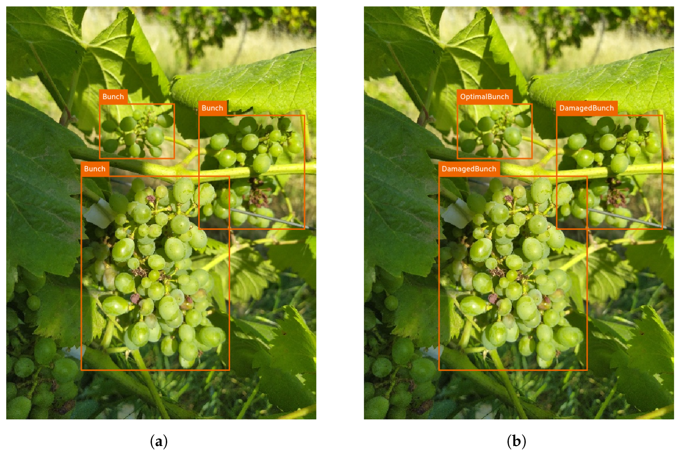
Two datasets were created with the same set of images and annotations, and the difference is in the classes of each dataset. This differentiation was performed to understand the complexity of each task:

• Grapevine bunch detection.
• Classification of the grapevine bunch as healthy or damaged.

In the Grapevine Bunch Detection Dataset (see https://doi.org/10.5281/zenodo.7717055, accessed on 7 March 2023), the “Bunch” class was used to annotate the grape bunches in each image. In Grapevine Bunch Condition Detection Dataset (see https://doi.org/10.5281/zenodo.7717014, accessed on 7 March 2023), the condition of the grape bunches was distinguished using the “OptimalBunch” and “DamagedBunch” classes. In this case, since automatic detection by DL models would be challenging if all damage variants were modeled, it was defined that a bunch is considered to be DamagedBunch when it has 10% or more of any physical damage; otherwise, it is considered OptimalBunch. The images were exported under the YOLO [35] format to train the YOLO models for each dataset. Figure 2 shows the same image with the annotations for each dataset (orange bounding boxes).

After annotating all objects, it was necessary to resize the images. Images with a resolution of 8000 × 6000 pixels introduce a large amount of data to be analyzed by the neural network, which increases the complexity and, inevitably, the processing time. Lowering the resolution to 720 × 540 pixels reduces the complexity while maintaining the aspect ratio at the cost of losing some detail in the image.

Next, it was checked that all images had at least one annotation, and images with no annotation were deleted. Thus, the size of each dataset decreased to 910 images since 58 images were removed.

Since DL training models require large amounts of data to perform well with new information, the dataset was increased using augmentation. By artificially increasing the size and variability of the dataset, the possibility of overfitting during training was reduced, so not performing this step may compromise the precision of the models [36].

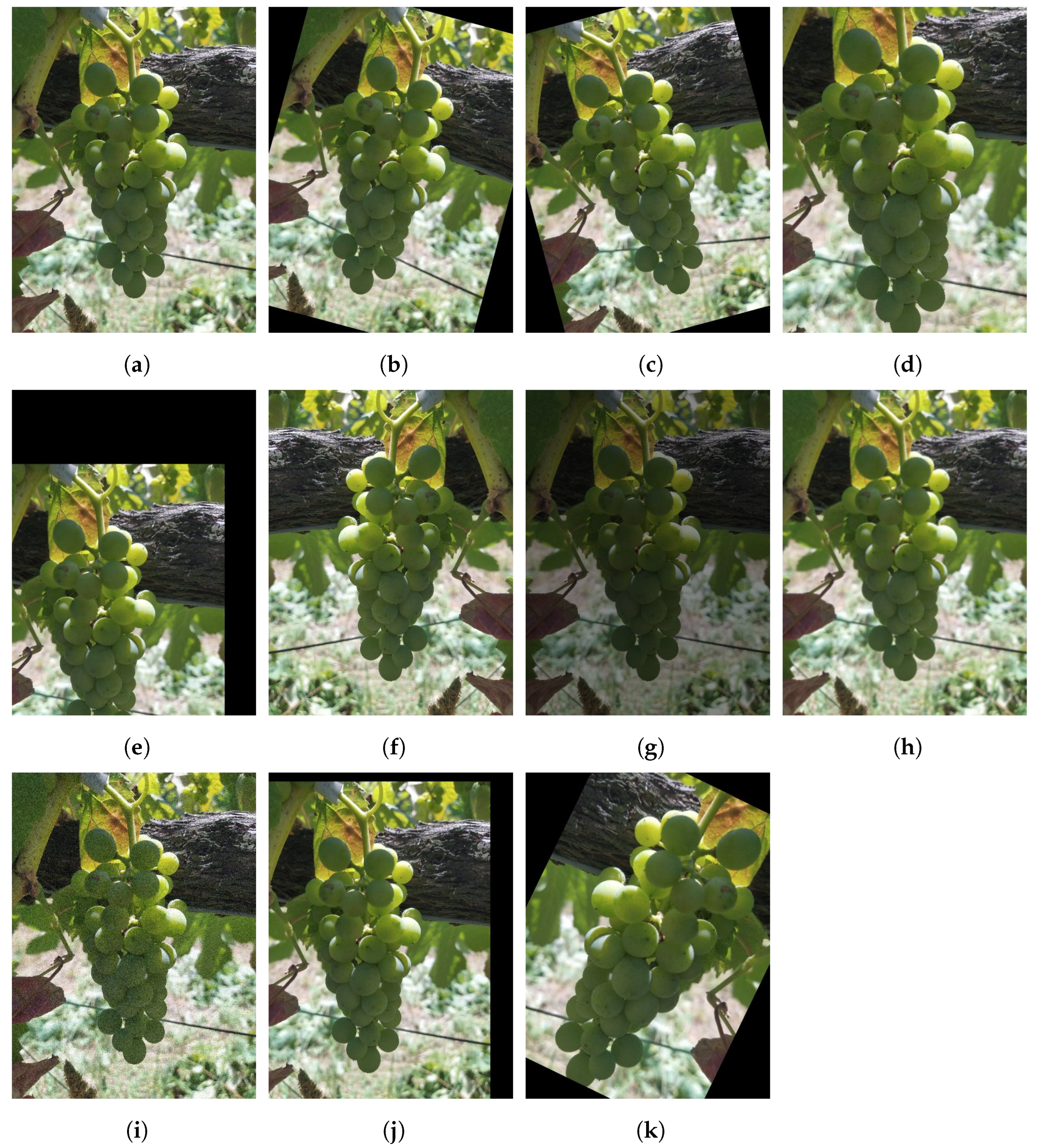
In this case, ten augmentation processes were chosen, so each original image resulted in ten new versions. The augmentation operations were carefully selected, and only the ones generating realistic vineyard images were applied.

Table 2. Description of the augmentation operations used to increase the original dataset.

Operation	Value	Description
Rotation	+15°	Rotates the image by +15°.
Rotation	−15°	Rotates the image by −15°.
Scale	random	Scales the image to a random value.
Translation	random	Translates the image by a random value.
Flip	-	Mirrors the image horizontally.
Multiply	random	Multiply all pixels in an image with a random value (makes images lighter or darker).
Blur	random	Blurs the image.
Noise	random	Adds Gaussian noise.
Combination 1	random	Random operation.
Combination 3	random	Random combination of three operations.

shows the description of the specified operations.

Figure 3 shows the augmentation operations performed on an original image, utilized in both datasets originating the same set of images. After augmentation, the size of each augmented dataset was 10,010 images (910 + 10 × 910).

Each dataset was divided into three sets: training (60%), validation (20%), and test (20%).

Table 3. Number of annotated objects per class in each set.

Dataset	Class	Train	Validation	Test	Total
Grapevine bunch detection	Bunch	6912	2329	2431	11,672
Grapevine bunch condition detection	OptimalBunch	4958	1637	1826	8421
	DamagedBunch	1954	692	605	3251

contains information about the number of annotated objects per class in the three sets.

Table 4. Number of images and annotated objects per class after and before augmentation.

Dataset	Classes	Images	Annotations
Original	Bunch	910	1066
	OptimalBunch	698	769
	DamagedBunch	277	297
Grapevine bunch detection	Bunch	10,010	11,672
Grapevine bunch condition detection	OptimalBunch	7678	8421
	DamagedBunch	3045	3251

shows the number of images and annotated objects per class after and before augmentation. The values shown after augmentation are not the original dataset multiplied by the number of augmentations performed since the annotations were reanalyzed to check their validity. Due to translations, two cases cause this change in values: (i) the translation leads to the detection being eliminated from the image, (ii) the part of the grape cluster that allows classifying as damaged is eliminated from the image.

2.3. Model Training

The final step in performing the detection of grape cluster conditions was the formation and deployment of models. To achieve the proposed goal, three of the latest YOLO models with different features were selected and benchmarked. These are some of the most recent models in the literature and present the best trade-off between accuracy and speed, which is fundamental for real-time applications.

YOLOv5 is designed to be more efficient and faster than previous versions while maintaining good performance in accuracy. The main advantage of YOLOv5 is Python-based PyTorch, which allows faster training [37].

YOLOv7, when released, was the best model for object detection, having a new architecture. This version is designed to be more accurate and robust than previous versions while maintaining real-time performance. YOLOv7 utilizes cross-scale-transformer (CST) to allow the model to handle objects at different scales [38].

YOLOR is a model inspired by the way humans acquire knowledge. This network is based on the YOLOv4 architecture and integrates implicit and explicit knowledge. When tacit knowledge is introduced into the network, it improves the performance [39].

The YOLO models (YOLOv5, YOLOv7, and YOLOR) were trained using Pytorch. For each model, the versions with the best results were chosen, regardless of the processing time.

Table 5. YOLO versions pre-trained checkpoints performance on large-scale public object detection dataset.

Model	Input Resolution (Pixels)	mAP 50 (%) Validation Set	AP 50 (%) Test Set	Speed (ms) Batch Size 32
YOLOv5x6 1	1280 × 1536	72.7	-	19.4
YOLOv7-E6E 2	1280 × 1280	-	74.4	18.7
YOLOR-CSP-X 3	1280 × 1280	-	73.1	5.5

¹ https://github.com/ultralytics/yolov5, accessed on 7 March 2023, ² https://github.com/WongKinYiu/yolov7, accessed on 7 March 2023, ³ https://github.com/WongKinYiu/yolor, accessed on 7 March 2023.

shows the characteristics of each selected version.

Each model was pre-trained with Microsoft’s COCO dataset [40]. Through transfer learning, fine-tuning was performed on the pre-trained models to detect grapevine bunches. The models were then individually trained with the developed datasets for 50 epochs with a batch size of 16 images and an input resolution of 640 × 640 pixels. Each training used the pre-trained weights and configuration the YOLO developers provided, all with an initial learning rate of 0.01. The models were trained using a NVIDIA GeForce 3090 graphics processing unit (GPU) with 24 gigabytes (GBs) of available memory.

The Fiftyone (see https://docs.voxel51.com/, accessed on 7 March 2023) platform was used to analyze the training results. This way, it was possible to observe the detections that the three networks could predict.

2.4. Model Evaluation

The neural network aims to identify objects, and the output consists of a list of bounding boxes, confidence levels, and classes. The evaluation of the neural network is carried out according to the predictions made by it.

Intersection over Union (IoU) is a metric that measures the area of overlap between the predicted bounding box and an object’s ground truth bounding box.

For the classification of detection as valid or invalid by comparing IoU with a given threshold t, to determine the type of detections, we use the concepts defined below:

• True Positive (TP): A valid detection of a ground truth bounding box, i.e., IoU $\ge t$;
• False Positive (FP): An invalid detection (incorrect detection of a non-existent object or incorrect detection of a ground truth bounding box), i.e., IoU $<t$;
• False Negative (FN): A missing detection of a ground truth bounding box;
• True Negative (TN): does not apply in object detection. There is no goal of finding the infinite bounding boxes in each image during object detection.

The precision × recall curve is a graphical representation of the trade-off between precision and recall. This metric plots a curve as confidence changes for each object class. The precision × recall curve is a metric to evaluate the performance of an object detection model, especially when the dataset is imbalanced and there are many more negative examples than positive examples. A poor object detector to increase recall needs to increase the number of detected objects, which implies an increase in the number of FP and a decrease in precision. A good object detector remains with high precision as recall increases when the confidence threshold varies. Therefore, an optimal object detector predicts only relevant objects (FP = 0) while finding all ground truth (FN = 0).

The Average Precision (AP) evaluates the performance of an object detector by calculating the area under the precision × recall curve. AP is the average precision of all recall values between 0 and 1. Therefore, a high area represents both high precision and recall.

The mean Average Precision (mAP) is a metric used for evaluating the overall performance of an object detector across all classes. The mAP is calculated as the average AP scores across multiple object classes in a dataset (or the area under the PR curve).

3. Results

3.1. Grapevine Bunch Detection Dataset

The Grapevine Bunch Detection Dataset’s results help to understand the complexity of grapevine bunch detection. The validation set results were generated using the same characteristics as the training input resolution 640 × 640 with batch size 16. Additionally, an IoU threshold of 50% was considered.

Table 6. Confidence threshold that optimizes the F1-score for each YOLO model with Grapevine Bunch Detection Dataset.

Models	Confidence Threshold (%)	F1 Score (%)
YOLOv5	42	93
YOLOv7	75	94
YOLOR	85	94

shows the confidence threshold value that maximizes the F1-score for each model in the validation set.

The confidence threshold values presented lead to the best balance between precision and recall, which maximizes the number of true positives and minimizes the value of FPs and FNs. All three models found their best F1-score above 90%. YOLOR presents the most promising values with higher confidence (94%).

Table 7. Detection results with the test set of Grapevine Bunch Detection Dataset considering different confidence thresholds.

Models	Confidence Threshold (%)	Precision (%)	Recall (%)	F1 Score (%)	mAP (%)
YOLOv5	>0	9	97	16	78
	42	97	91	94	75
YOLOv7	>0	5	99	9	81
	75	98	90	94	77
YOLOR	>0	21	97	34	81
	85	98	86	92	75

shows the results with the test set considering different confidence thresholds. The inference was performed for the 0% confidence threshold and the confidence threshold value that maximizes the F1-score in the validation set, also considering an IoU threshold of 50%.

Lower confidence rates cause FPs to increase and FNs to decrease. Therefore, a lower confidence rate causes a decrease in precision caused by an increase in FPs and an increase in recall caused by a decrease in FNs.

The results obtained for the confidence threshold greater than 0% show that this approach has no applicability, resulting only in a good point of comparison for the mAP. The high values of recall indicate that, practically, all grape bunches are detected. However, the Precision reveals that there are quite a few incorrect grape bunch detections, and a relatively low value of the F1-score is expected.

By assuming the confidence threshold value that maximizes the F1-score, there is a considerable increase in accuracy and F1-score at the cost of a slight decrease in recall and mAP. The accuracy values are above 95%, i.e., the models rarely misidentify areas of the image as grape bunches. However, a higher number of grape bunches failed to be detected. The F1-score higher than 90% demonstrates that the balance between accuracy and recall is much higher. The mAP value reveals that the variation in the confidence threshold causes some impact on the recall and precision.

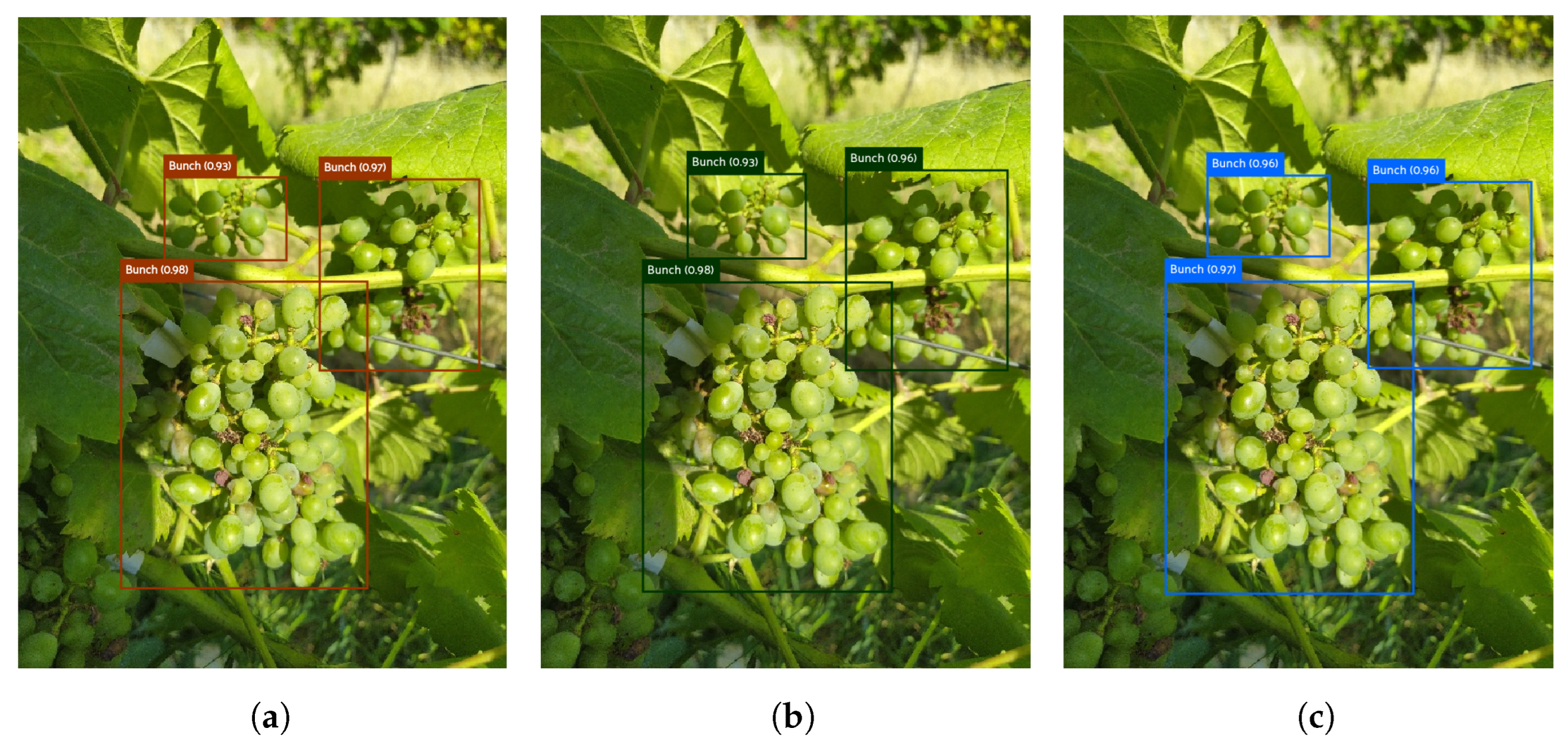
Overall, the results for the three models are promising and similar. YOLOv7 has the best performance in most metrics. To better understand the outcome of some metrics, it was necessary to observe the model detections on the test set images. Figure 4 presents the results of the ability of each YOLO version to detect grape bunches in a test set image. The models had a good response, despite the complexity of the image, i.e., three grape bunches of different sizes with different light conditions along the bunch.

Despite the good results in the predictions of the grape bunch conditions, it is relevant to analyze and understand why FPs and FNs occurred to implement solutions. The presence of FPs influences the value of the metric precision; if FPs are mitigated, the value of the precision increases. Figure 5 presents two images from the test set with FPs that occurred in the three models.

These two examples resume the cases where the models generate FPs with the developed dataset:

• Figure 5a–c present the results of the trained models to a case with two bounding boxes very approximated. The models were not able to detect the two bunches. The result is a bounding box around the two bunches, causing a false positive (IoU < 0.5).
• Figure 5d–f show the results of the trained models to a case with a small grape bunch blurred in the background. Due to the complexity of the detection was chosen not to annotate this grape bunch. However, all three models have the ability to detect grape bunches under these conditions.

Furthermore, analyzing the FNs to understand the reason for the recall outcome is relevant. If FNs are mitigated, the value of recall increases. Figure 6 shows the results in two different images of the set of tests with FNs that occurred in the three models.

These two examples resume the cases where the models generate FNs with the developed dataset:

• Figure 6a–c present the results of the trained models to a case with two bunches of grapes annotated, one bunch in the center of the image and another near the top left corner with a peculiar structure. The models did not predict the second bunch of grapes, resulting in a false negative.
• Figure 6d–f show the results of the trained models to a case with three bunches overlapping. None of the models could detect the three different grape bunches. However, the predicted detections are true positives.

3.2. Grapevine Bunch Condition Detection Dataset

The evaluation of the results from the dataset Grapevine Bunch Condition Detection helps to understand the complexity of detecting the grapevine bunch condition. The validation set results were generated using the same characteristics as the training input resolution 640 × 640 with batch size 16. Additionally, an IoU threshold of 50% was considered.

Table 8. Confidence threshold that optimizes the F1-score for each YOLO model with Grapevine Bunch Condition Detection Dataset.

Models	Confidence Threshold (%)	F1 Score (%)
YOLOv5	52	89
YOLOv7	72	88
YOLOR	79	89

shows the confidence threshold value that maximizes the F1-score for each model in the validation set.

The results show an F1-score above 85% for all three models and a superior confidence threshold with YOLOv7 and YOLOR.

Table 9. Detection results with the test set of Grapevine Bunch Condition Detection Dataset considering different confidence thresholds.

Models	Confidence Threshold (%)	Classes	Precision (%)	Recall (%)	F1 Score (%)	mAP (%)
YOLOv5	>0	OptimalBunch	9	96	16	74
		DamagedBunch	6	91	10
	52	OptimalBunch	94	90	92	72
		DamagedBunch	98	87	93
YOLOv7	>0	OptimalBunch	3	97	7	76
		DamagedBunch	3	94	6
	75	OptimalBunch	95	85	90	72
		DamagedBunch	96	86	91
YOLOR	>0	OptimalBunch	21	95	34	76
		DamagedBunch	15	88	26
	76	OptimalBunch	94	83	88	76
		DamagedBunch	97	85	91

shows the results with the test set considering different confidence thresholds. The inference was performed for the 0% confidence threshold and the confidence threshold value that maximizes the F1-scores in the validation set, also considering an IoU threshold of 50%.

As with the grape bunch detection dataset, the results obtained for the confidence threshold greater than 0% show that this approach has no applicability, only for mAP comparison. The recall higher than 85% shows that quite a few grape bunches are detected and correctly classified according to the bunch conditions. However, a precision lower than 25% indicates that there are quite a few incorrect detections of grape bunches, which are also expected to have a low F1-score value.

When assuming the confidence threshold value that maximizes the F1-score, there is a considerable increase in the precision and F1-score at the cost of a slight decrease in recall and mAP. The precision values are above 85%, which means that the models rarely make wrong detections. However, a higher number of damaged and optimal grape bunches fail to be detected. The F1-score above 85% demonstrates that the balance between precision and recall is much higher, while the mAP value changes little with the threshold change.

Overall, the results for the three models are promising and similar. The results of the metrics for YOLOv5 are approximated for both classes. The results for YOLOv7 and YOLOR show a slight decrease in precision for the DamagedBunch class and a slight decrease in recall for the OptimalBunch class, meaning that the DamagedBunch class has a higher ratio of FPs and the OptimalBunch class has a higher percentage of FNs. This may mean that OptimalBunch detections may be misidentified as DamagedBunch. Figure 7 shows the confusion matrixes for each model to better understand the mismatch between classes.

The confusion matrix presents the performance of a model by resuming the number of correct and incorrect predictions. The three models have similar results, with the majority of the predicted labels corresponding to the true labels. Analyzing the cases of mismatch between classes, there are few incorrect predictions, i.e., a low percentage of mismatches between classes identifying healthy or damaged bunches.

To better understand the results of some metrics, it was necessary to observe the detections of the models on the test set images. Figure 8 presents the results of the ability of each YOLO version to detect the state of each bunch of grapes in a test set image. The models had a good response despite the complexity of the image, i.e., three grape bunches of different conditions, dimensions, and light conditions along the bunch.

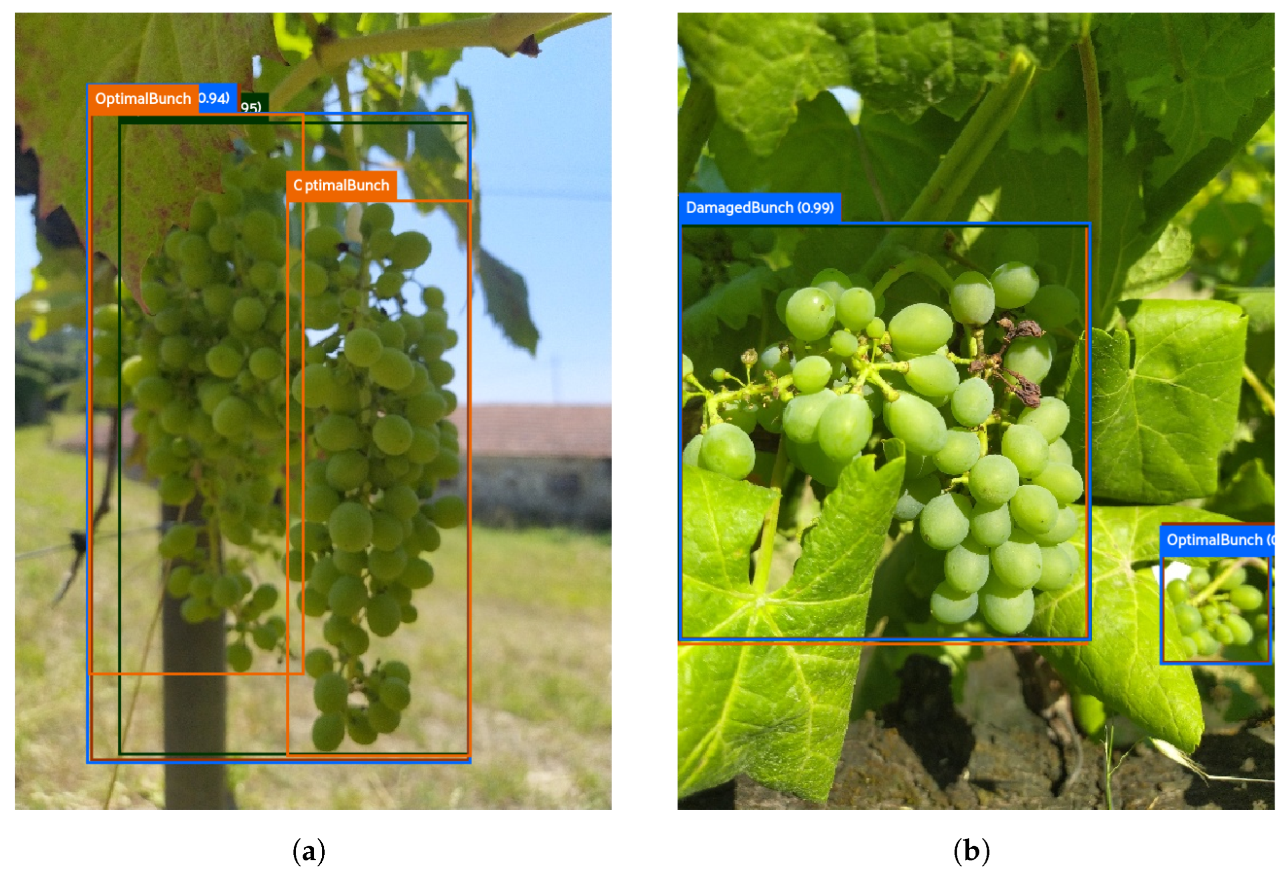
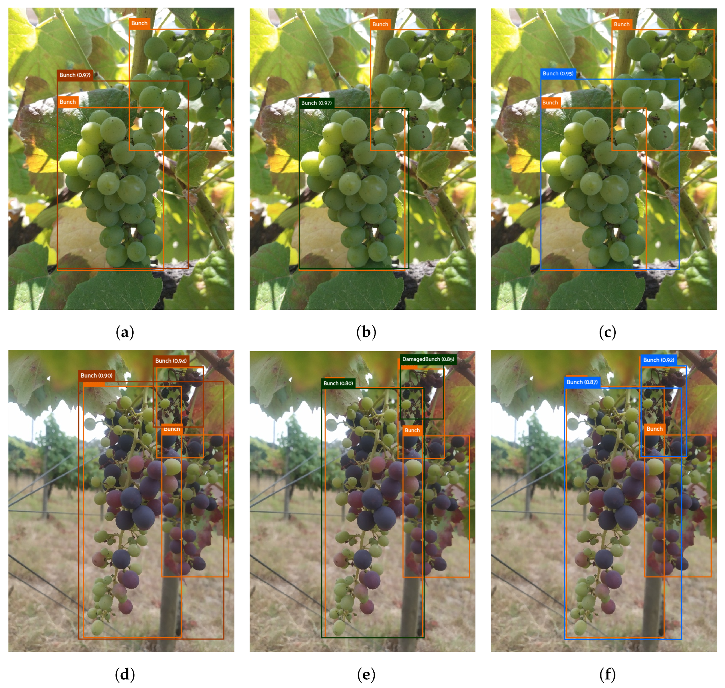
Despite the good results in the predictions of the grape bunch conditions, it is relevant to analyze and understand why FPs and FNs occurred to implement solutions. The presence of FPs influences the value of the metric precision; if FPs are mitigated, the value of the precision increases. Figure 9 presents two images of the test set with common FPs to the three models.

These two cases illustrate errors related to the detection of the bunches, which coincide with the results from the Grapevine Bunch Detection Dataset (compare with Figure 5):

• Figure 9a presents that the models detect only one bunch when two bunches are approximated (the bounding box includes the two grape bunches).
• Figure 9b presents a small and blurred grape bunch, which all models could predict.

Apart from FPs to detect the bunches, Figure 10 shows two other cases with FPs that occurred in the three models when they failed to classify the condition of the grape bunches.

This example resumes the cases of FPs generated by the models when they failed to classify the condition of the bunch with the developed dataset. Figure 10a–c show a complex case of detection because of the overlapping of grape bunches. The models predicted the optimal bunch, which was not annotated; however, the models could not detect the damaged bunch, which is more visible.

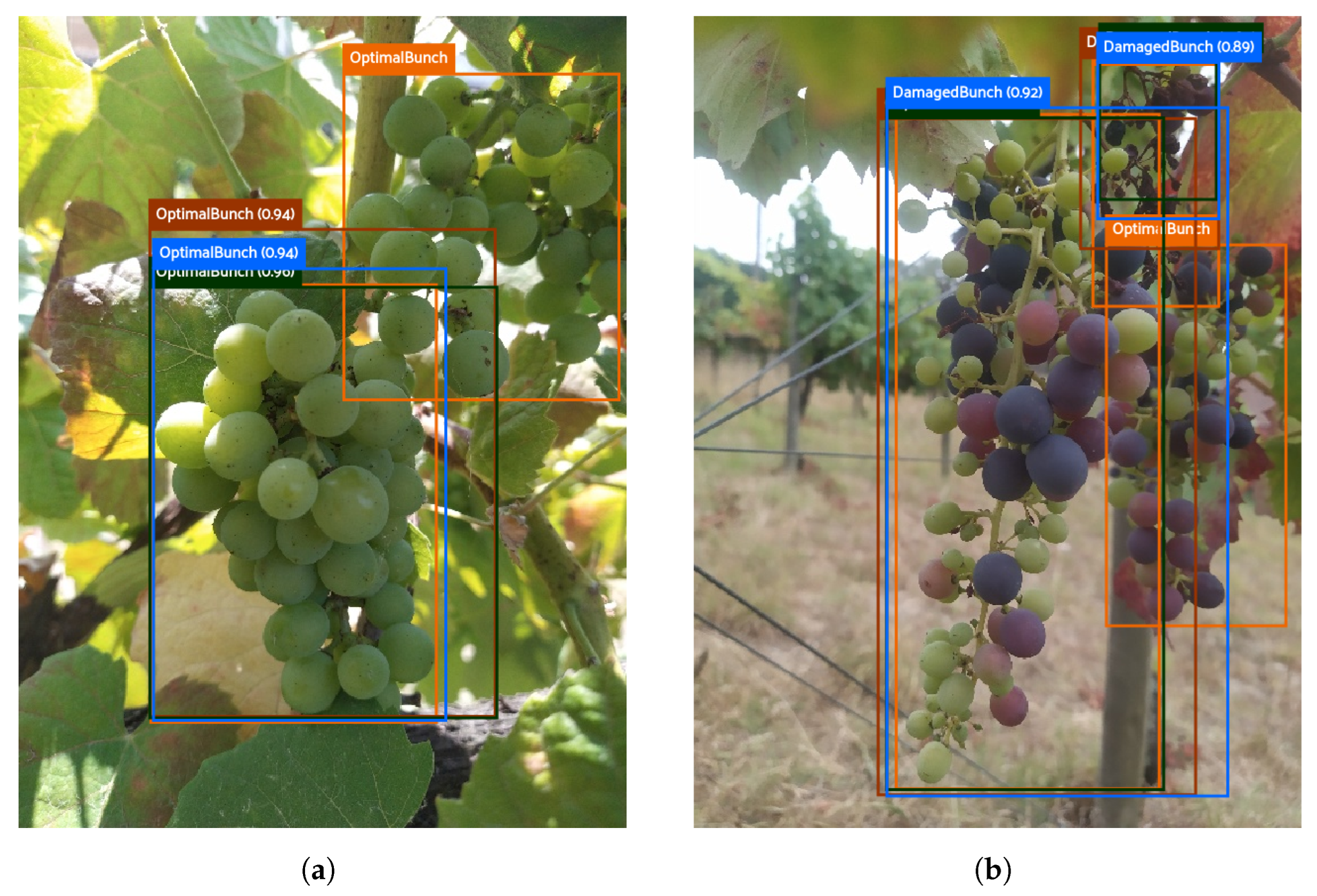
Furthermore, analyzing the FNs to understand the reason for the recall outcome is relevant. If FNs are mitigated, the value of recall increases. Figure 11 shows two FN cases in the three models.

These two cases illustrate errors related to the detection of the bunches, which coincide with the results from the dataset Grapevine Bunch Detection (compared with Figure 6):

• Figure 11a shows that none of the trained models could detect the two bunches possible because of the location and structure of the grape bunch.
• Figure 11b shows three bunches with different conditions overlapping, where the more overlapped bunch was not detected.

Apart from FNs to detect bunches, Figure 12 presents two other cases with FNs that occurred in the three models when they failed to classify the condition of the grape bunches. These two examples resume the cases of FNs generated by the models when they failed to classify the condition of the bunch with the developed dataset:

• Figure 12a–c present the results of the trained models to a case with two bunches of grapes in different conditions. The models could not predict and/or classify bunches in the image. YOLOv5 can localize the two bunches but fails at classifying the damaged bunch. YOLOv7 only predicted and correctly typed one of the bunches (OptimalBunch). YOLOR only predicted one of the bunches and failed to classify it (DamagedBunch). The three models failed to predict the DamagedBunch, resulting in FNs.
• Figure 12d–f present the results of the trained models to a case with a bunch with a small percentage of damaged grapes. None of the models could classify the bunch as damaged, resulting in FNs.

4. Discussion

The Grapevine Bunch Detection Dataset’s results on the test set were satisfactory in grape bunch detection when using the confidence threshold that maximizes the F1-score on the validation set. Using the confidence threshold that maximizes the F1-score became an essential step that harmonized the metric results, leading to a significant decrease in FP. The three models tested show similar results, with YOLOv7 achieving the best performance in grape cluster detection. The models can detect grape bunches in several complex scenarios, even in complex scenarios considering occlusions, overlaps and variations in lighting conditions. FP happens when bunches are extraordinarily close or overlapping (the models detect a bunch that includes both) and with small unannotated bunches. On the other hand, FNs occur when bunches are close to the edges, have a different structure than expected, or are overlapping. The YOLOv7-based grape cluster detector achieved precision of 98%, recall of 90%, F1-score of 94% and mAP of 77%.

The Grapevine Bunch Condition Detection Dataset’s results in the test set were satisfactory in detecting grape bunches condition when using the confidence threshold that maximizes the F1-score in the validation set, and the results between the two classes, with the DamagedBunch class obtaining the best values. The three models present similar results and could detect grape bunches conditions in different scenarios, even with bunches with a low percentage of damaged grapes (and the variations mentioned in the other dataset). Regarding errors about the condition of the bunches, the presence of FPs happens when damaged bunches overlap optimal bunches. On the other hand, FNs occur in complex cases with low visibility of the bunch conditions or bunches, which is difficult to define if they are damaged.

The results from the developed datasets are similar, with slightly decreasing metrics in the second dataset. These analyses reveal that the most complex task is to detect grape bunches, which lead to a mAP under 85%. The other metrics (precision, recall, and F1-score) present results over 85%.

Comparing these results with those of different authors is essential to understand the results’ relevance and the potential aspects that could be improved. Firstly, the results from Grapevine Bunch Detection Dataset were compared with articles that only detect the bunches (most articles only realize this task without analyzing the condition of the grapes). The Grapevine Bunch Condition Detection Dataset was compared with articles that detect and classify the bunches by the state of the berries (

Table 10. Comparison between the proposed models and the state-of-the-art DL for grapevine bunch detection and classification based on the health state.

Application	State-of-the-Art	Results
Grape Bunch detection	Deng et al. [23]	N/A
Grape Bunch detection	Heinrich et al. [24]	N/A
Grape Bunch detection	Sozzi et al. [26]	48.90% (Accuracy)
Grape Bunch detection	Aguiar et al. [25]	66.96% (mAP)
Grape Bunch detection	Sozzi et al. [28]	79.60% (mAP)
Grape Bunch detection	Santos et al. [22]	84.00% (F1-Score)
Grape Bunch detection	Yin et al. [20]	89.53% (AP)
Grape Bunch detection	Li et al. [27]	90.47% (F1-Score)
Grape Bunch detection	Ghiani et al. [21]	92.78% (mAP)
Grape Bunch detection	Proposed	94.00% (F1-Score)
Grape Bunch detection and classification	Miranda et al. [30]	93.80% (Accuracy)
Grape Bunch detection and classification	Proposed	96.00% (Precision)
Grape Bunch detection and classification	Bömer et al. [8]	96.26% (Precision)

).

The YOLOv7 and YOLOR models trained with the Grapevine Bunch Detection Dataset outperformed those presented by Santos et al. [22], Aguiar et al. [25] and Sozzi et al. [28], comparing the results from the common metrics between the researches. Concerning the results presented by Li et al. [27], these are inferior in all metrics except mAP. Despite the satisfactory results, the dataset used by Yin et al. [20] was not robust, and the results can be inferior in other scenarios. Ghiani et al. [21] present only mAP to evaluate the performance of the formed model, making it problematic to analyze the model’s advantages because it only uses one metric for performance evaluation.

The three models trained in the Grapevine Bunch Detection Condition Dataset achieved similar results to those presented by Bömer et al. [8].

Sozzi et al. [26] and Miranda et al. [30] only utilized the accuracy metric, which is not usually used for object detection. There are no common metrics between this study and the referenced articles.

Table 10 compiles all the results found in the state of the art as well as the results obtained in this paper, for comparison of the models used. This paper can detect biophysical lesions in the grape bunches (with a minimum of 10% lesion area), utilizing two of the most recent YOLO models, which enables a comparison between more models, enriching the state of the art. The algorithms work for both varieties, with no change in the model performance between white and red varieties. The other articles in the state of the art detect the grape bunch without detecting the biophysical lesions.

5. Conclusions

This work focuses on detecting lesions on grape clusters, unlike most works that only predict lesions on leaves. However, the most pernicious lesions occur at the fruit level, which makes this work innovative and pertinent. The work developed can be implemented in any vineyard monitoring system, helping vineyard managers to improve harvest efficiency and quality.

In this way, this paper presents three pre-trained YOLO models for identifying the grape bunches and classifying the conditions (optimal or damaged). For this purpose, two similar datasets were created with 10,010 images of grape bunches with annotations with different classes and then augmented, as DL training models require large data.

The results obtained for identifying bunches were similar between models and promising, with the YOLOv7 model presenting the best performance, achieving 98% of precision, 90% of recall, 94% of F1-score and 77% mAP when selecting the confidence threshold that maximizes the F1-score in the validation set. For the classification task, the results were similar between the three models, with YOLOv5 being the best one, achieving 72% of mAP. The analysis of the FPs and FNs revealed the three models’ common difficulties:

• Identifying individual bunches when they are significantly closer;
• Detecting bunches with peculiar structures;
• Predicting overlapped bunches;
• Classifying damaged bunches in difficult conditions of visibility.

In both situations, the models worked independently of the variety. Furthermore, the phenological state in which the images were captured does not allow us to verify changes in the performance of the models between white and red varieties.

Regarding the detection of diseases of grapevines, most studies focus on detecting leaf diseases since it is preferable and ideal to adopt preventive strategies and act before the bunches appear to avoid compromising production. However, this approach does not exclude the possibility of the disease appearing later. Therefore, monitoring and detecting diseases are crucial throughout the entire plant cycle.

The detection and assessment of biophysical lesions of grapevine bunches is still a relatively under-studied area, so it is crucial to define the future work that can be divided into three main steps. The first step is to enlarge the dataset with images of grape bunches in more advanced phenological stages, which allows the comparison between white and red varieties. The use of public datasets may be relevant to increase variability and reduce some possible overfitting of the models. The following steps are to analyze, test and compare other DL models to see which one has the best performance is obtained and possibly complement these algorithms with spectral information for the recognition relevant parameters, such as, for example, disease detection. In addition, segmenting and counting the berries in each bunch of grapes according to their lesions allows the accurate prediction of vine production.