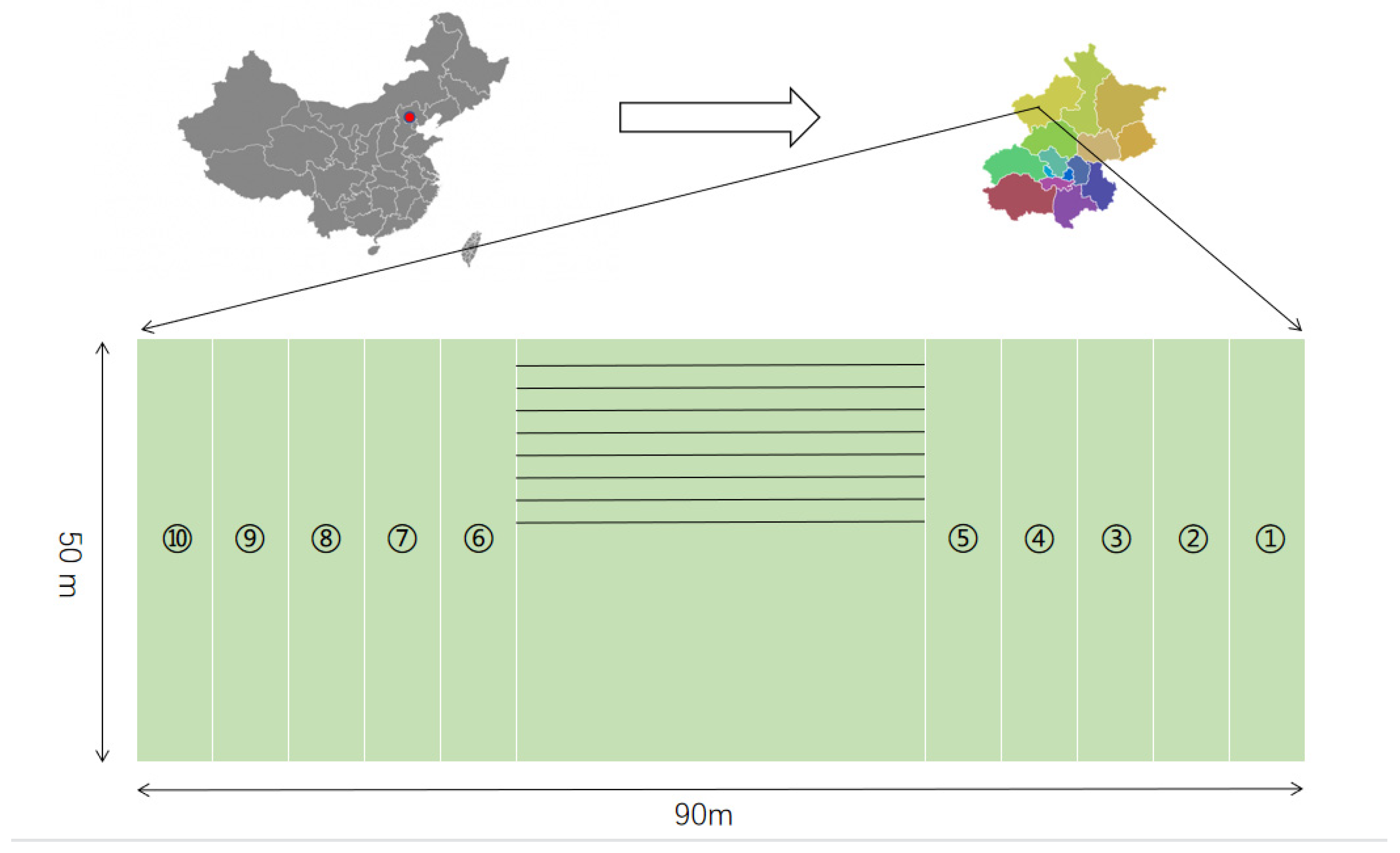
Figure 1.
Experimental plots. Note: ①, Zhongmai 175; ②, Lunxuan 987; ③, Shixin 828; ④, Lunxuan 518; ⑤, Zhongmai 12; ⑥, Zhongmai 11; ⑦, Wanmai 38; ⑧, Zhongmai 13; ⑨, Jingdong 8; ➉, Jimai 20. These are the varieties of wheat. The m stands for meter.
Figure 1.
Experimental plots. Note: ①, Zhongmai 175; ②, Lunxuan 987; ③, Shixin 828; ④, Lunxuan 518; ⑤, Zhongmai 12; ⑥, Zhongmai 11; ⑦, Wanmai 38; ⑧, Zhongmai 13; ⑨, Jingdong 8; ➉, Jimai 20. These are the varieties of wheat. The m stands for meter.
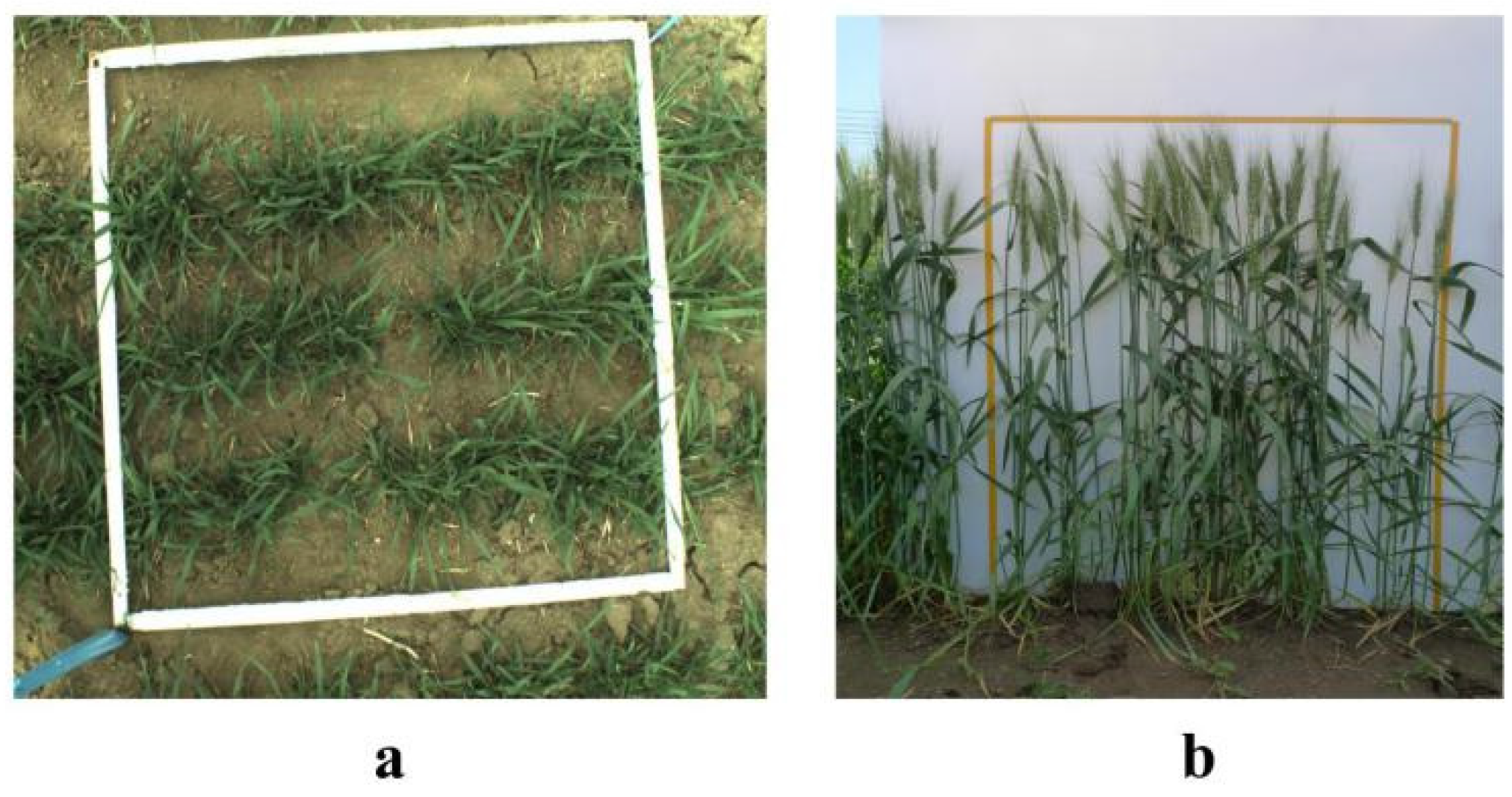
Figure 2.
(a) Canopy image at the seedling stage; (b) side image at the post-seedling stage.
Figure 2.
(a) Canopy image at the seedling stage; (b) side image at the post-seedling stage.
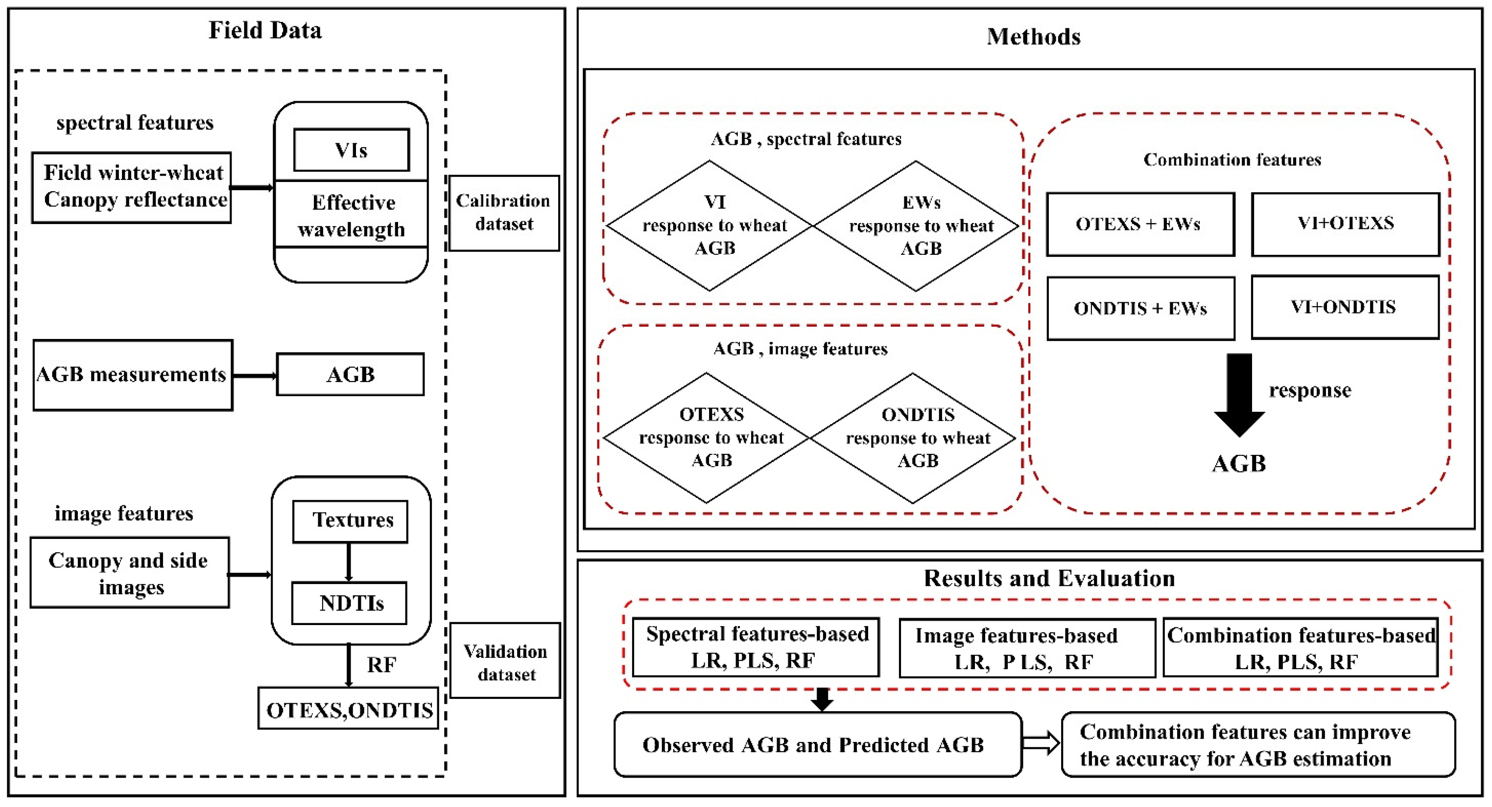
Figure 3.
Experiment methodology.
Figure 3.
Experiment methodology.
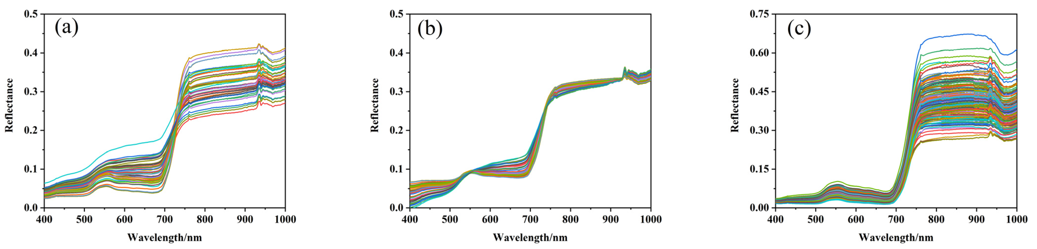
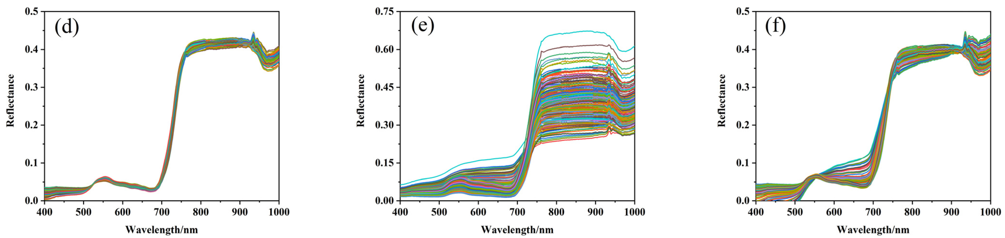
Figure 4.
Reflectance spectra of the winter wheat canopy at different growth stages. Omni-spectral data in (a) the seedling stage, (b) the post-seedling stage, and (c) all stages, as well as pre-spectrum data in (d) the seedling stage, (e) post-seedling stage, and (f) all stages.
Figure 4.
Reflectance spectra of the winter wheat canopy at different growth stages. Omni-spectral data in (a) the seedling stage, (b) the post-seedling stage, and (c) all stages, as well as pre-spectrum data in (d) the seedling stage, (e) post-seedling stage, and (f) all stages.
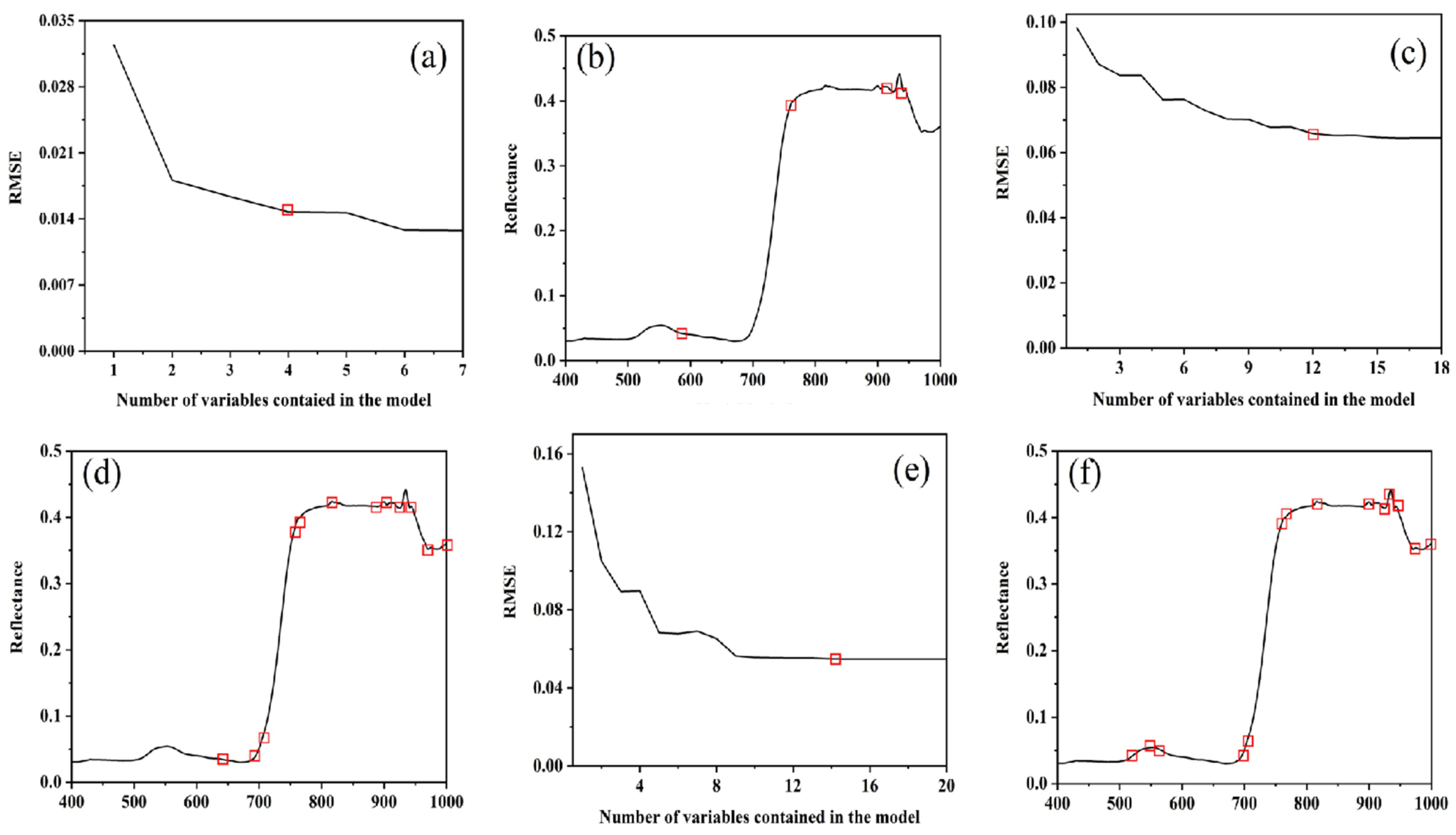
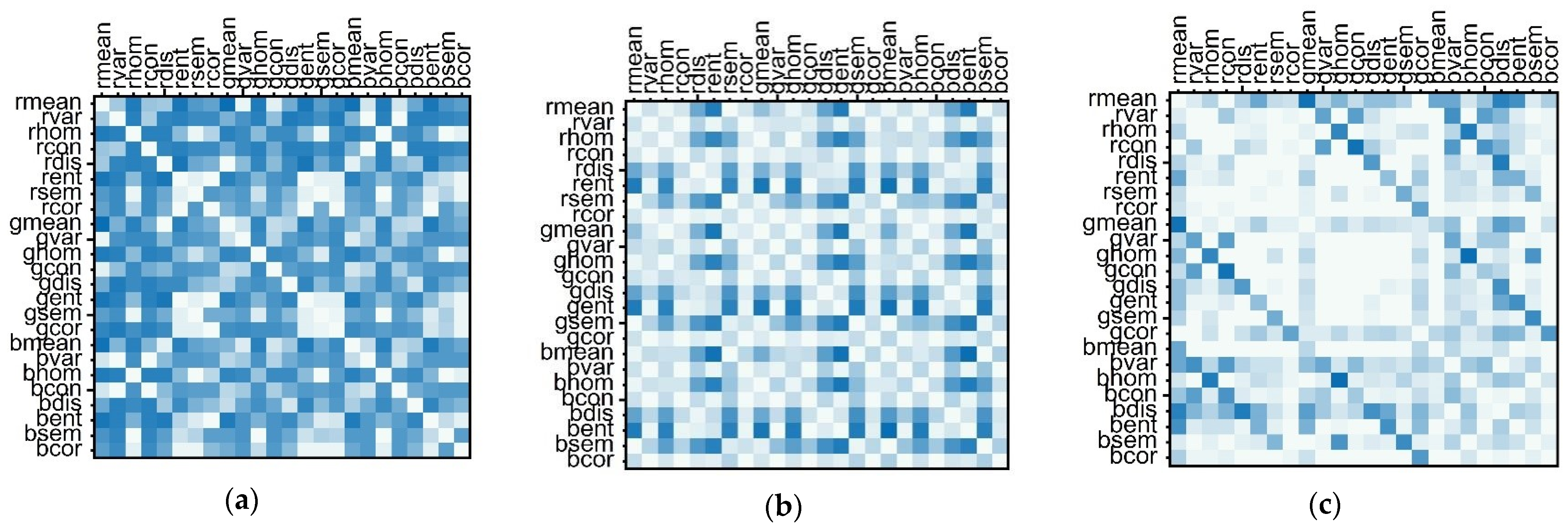
Figure 5.
Reflectance spectra of the winter wheat canopy at the seedling stage: (a–c) show the number of variables contained in the model in the seedling stage, post-seedling stage, and at all stages, respectively; (d–f) show the wavelength in the seedling stage, post-seedling stage, and at all stages, respectively. A square (□) represents the number of the effective wavelength.
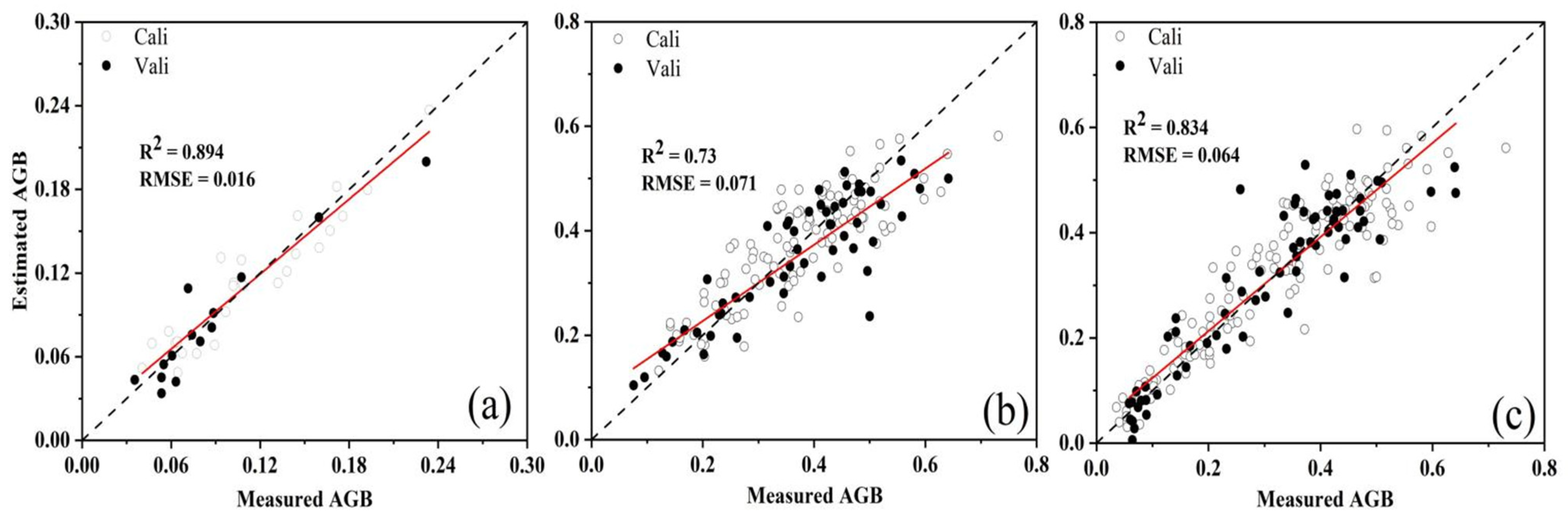
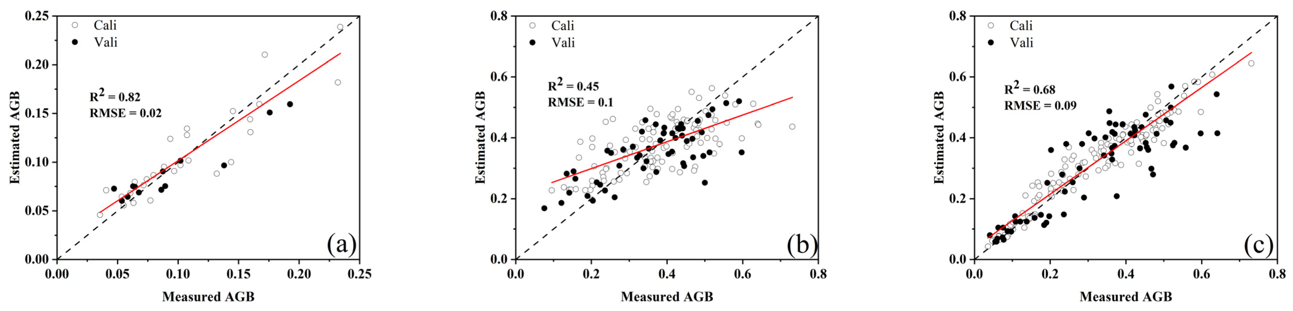
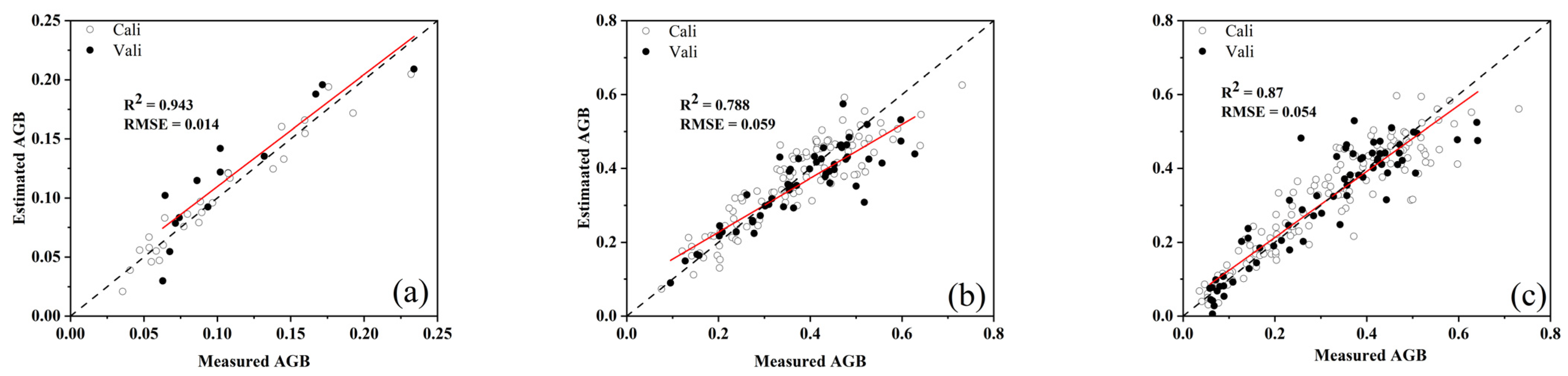
Figure 6.
Validation of aboveground biomass (AGB) estimation models established by best performing effective wavelengths vs. AGB for the following stages: (a) seedling, (b) post-seedling, (c) all stage.
Figure 6.
Validation of aboveground biomass (AGB) estimation models established by best performing effective wavelengths vs. AGB for the following stages: (a) seedling, (b) post-seedling, (c) all stage.
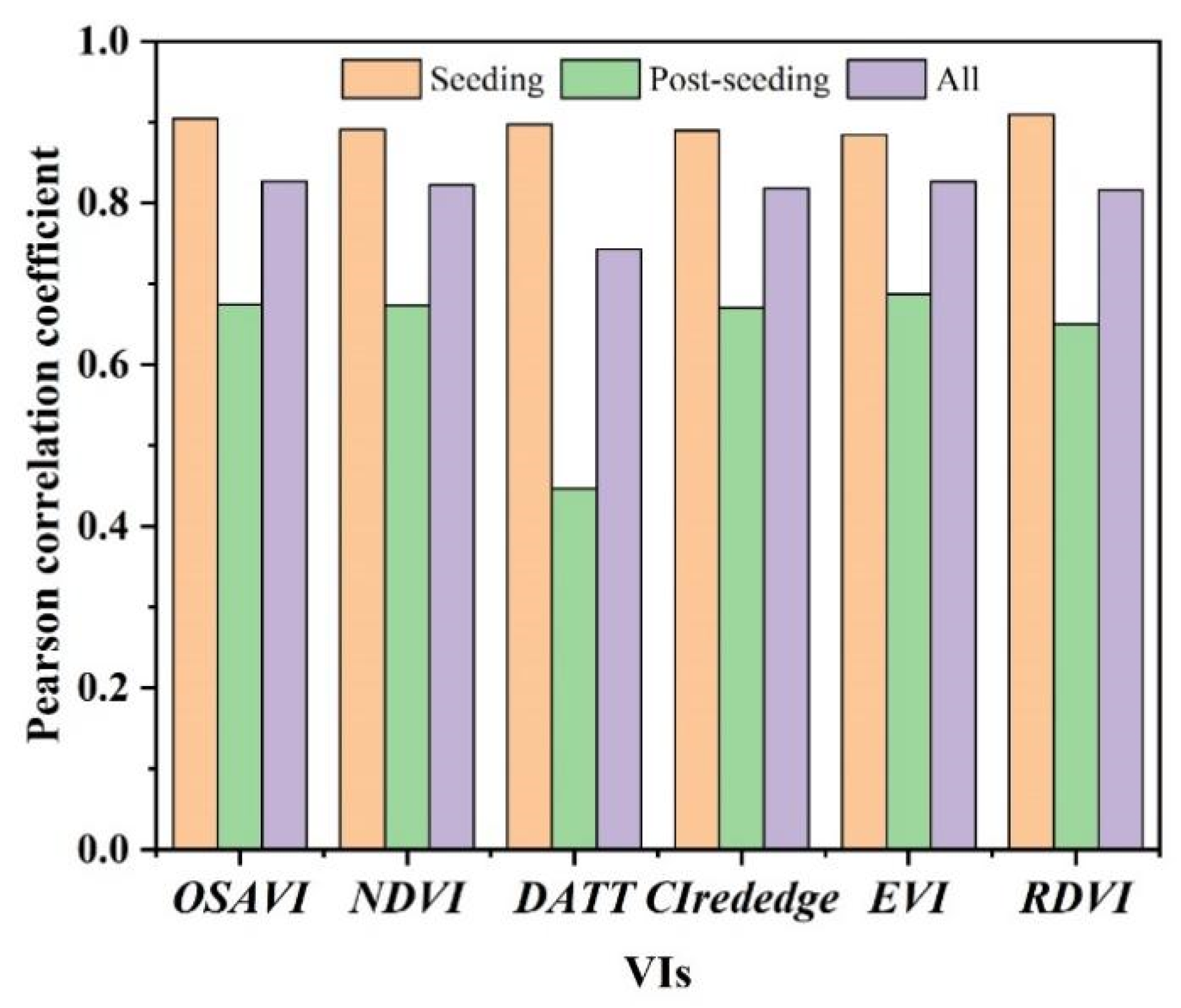
Figure 7.
Pearson correlation coefficient between vegetation indices and aboveground biomass.
Figure 7.
Pearson correlation coefficient between vegetation indices and aboveground biomass.
Figure 8.
Validation of aboveground biomass (AGB) estimation models established by best performing vegetation index vs. AGB for the following stages: (a) seedling, (b) post-seedling, (c) all stages.
Figure 8.
Validation of aboveground biomass (AGB) estimation models established by best performing vegetation index vs. AGB for the following stages: (a) seedling, (b) post-seedling, (c) all stages.
Figure 9.
Validation of aboveground biomass (AGB) estimation models established by best performing optimal texture subset vs. AGB for the following stages: (a) seedling, (b) post-seedling, (c) all stages.
Figure 9.
Validation of aboveground biomass (AGB) estimation models established by best performing optimal texture subset vs. AGB for the following stages: (a) seedling, (b) post-seedling, (c) all stages.
Figure 10.
R2 value of the normalized differential texture index-based linear regression models for estimating aboveground biomass at the (a) seedling stage, (b) post-seedling stage, and (c) across all stages.
Figure 10.
R2 value of the normalized differential texture index-based linear regression models for estimating aboveground biomass at the (a) seedling stage, (b) post-seedling stage, and (c) across all stages.
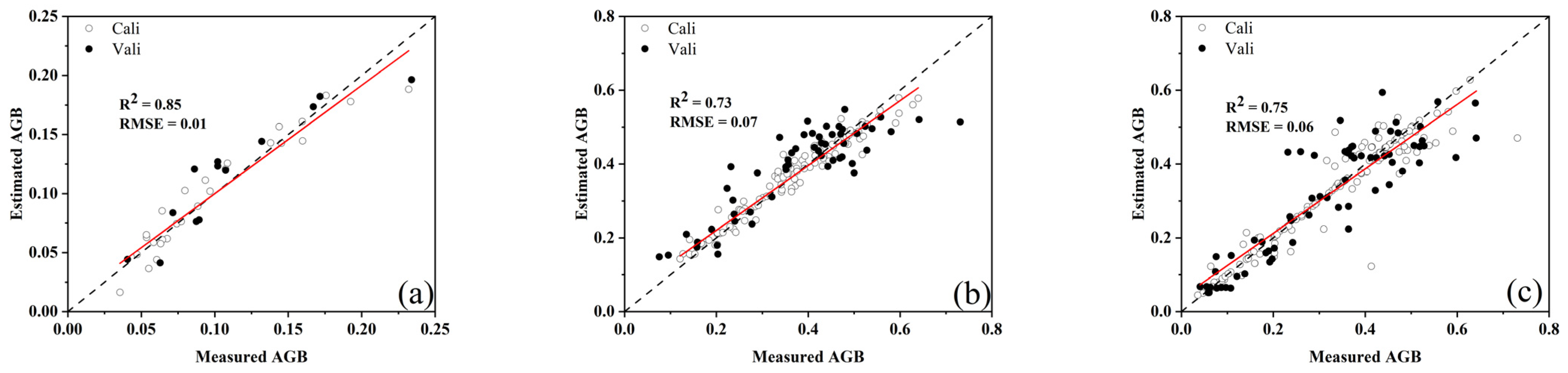
Figure 11.
Validation of aboveground biomass (AGB) estimation models established by best performing optimal normalized difference texture index subset vs. AGB for the following stages: (a) seedling, (b) post-seedling, (c) all stages.
Figure 11.
Validation of aboveground biomass (AGB) estimation models established by best performing optimal normalized difference texture index subset vs. AGB for the following stages: (a) seedling, (b) post-seedling, (c) all stages.
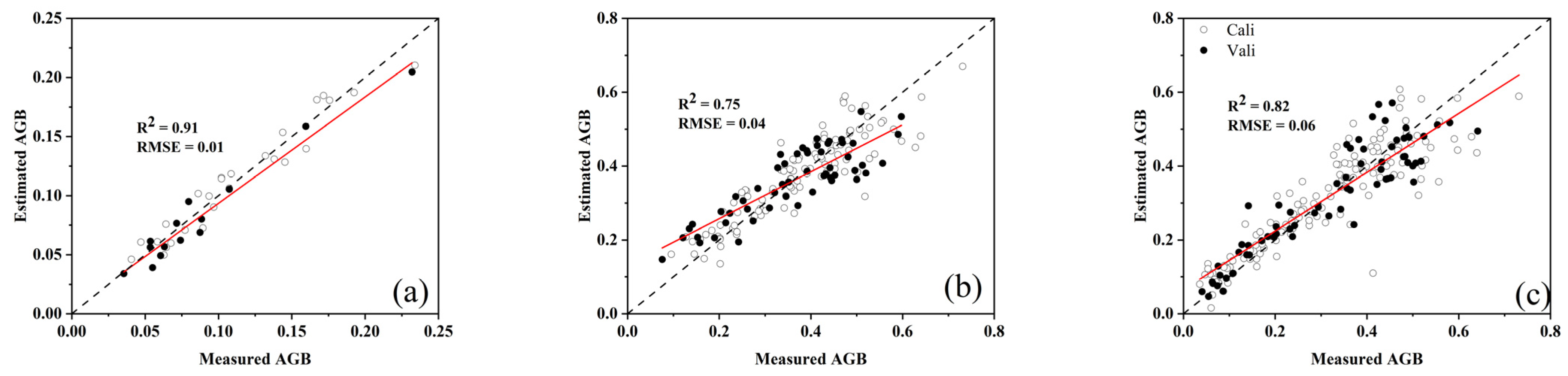
Figure 12.
Validation of aboveground biomass (AGB) estimation models established by best performing optimal normalized difference texture index subset vs. AGB for the following stages: (a) seedling, (b) post-seedling, (c) all stages.
Figure 12.
Validation of aboveground biomass (AGB) estimation models established by best performing optimal normalized difference texture index subset vs. AGB for the following stages: (a) seedling, (b) post-seedling, (c) all stages.
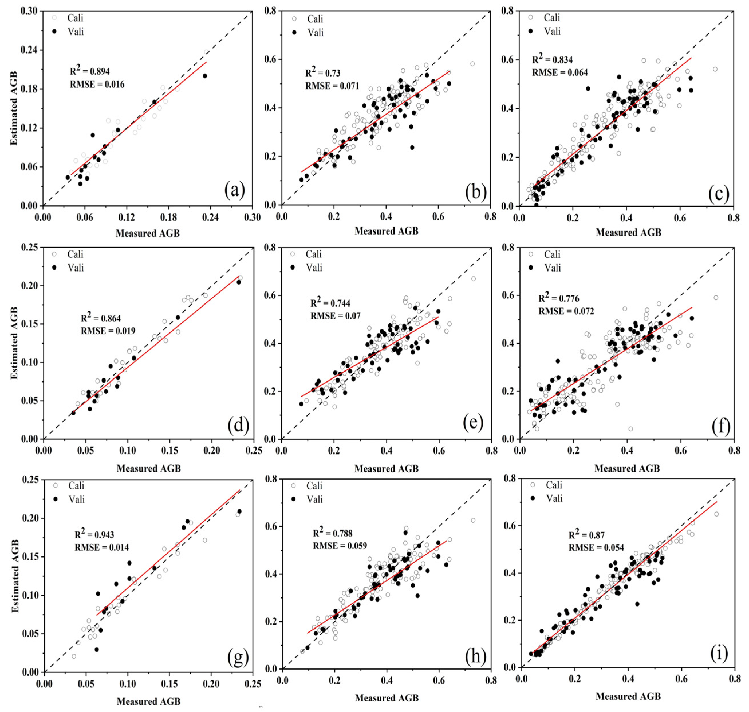
Figure 13.
Validation of aboveground biomass (AGB) estimation models established by best performing spectral, image, and combination features. Effective wavelengths for the following stages: (a) seedling, (b) post-seedling, (c) all stages. ONDTIS for the following stages: (d) seedling, (e) post-seedling, (f) all stages. OTEX + effective wavelengths for the following stages: (g) seedling, (h) post-seedling, (i) all stages.
Table 1.
Descriptive statistics of aboveground biomass measurements at different growth stages.
Table 1.
Descriptive statistics of aboveground biomass measurements at different growth stages.
| Dataset | Stage | Samples | Max/kg | Mean/kg | Min/kg | Std/kg |
|---|
| Calibration | Seedling | 27 | 0.23 | 0.102 | 0.04 | 0.05 |
| | Post-seedling | 107 | 0.73 | 0.37 | 0.08 | 0.13 |
| | All | 134 | 0.73 | 0.317 | 0.04 | 0.16 |
| Validation | Seedling | 13 | 0.232 | 0.106 | 0.047 | 0.054 |
| | Post-seedling | 53 | 0.641 | 0.372 | 0.121 | 0.125 |
| | All | 66 | 0.639 | 0.317 | 0.047 | 0.156 |
Table 2.
Selected vegetation indices in this study for aboveground biomass estimation.
Table 2.
Selected vegetation indices in this study for aboveground biomass estimation.
| Vegetation Index | Formula | Reference |
|---|
| OSAVI |
| [23] |
| NDVI |
| [24] |
| DATT |
| [25] |
| CI red edge |
| [26] |
| EVI |
| [27] |
| RDVI |
| [28] |
Table 3.
Aboveground biomass estimates using selected effective wavelengths at different growth stages.
Table 3.
Aboveground biomass estimates using selected effective wavelengths at different growth stages.
| | LR | RF | PLS |
|---|
| |
|
|
|
|
|
|
|
|
|
|
|
|
|---|
| Seedling | 0.89 | 0.01 | 0.89 | 0.01 | 0.96 | 0.01 | 0.84 | 0.02 | 0.91 | 0.01 | 0.89 | 0.01 |
| Post-seedling | 0.72 | 0.06 | 0.73 | 0.07 | 0.92 | 0.03 | 0.69 | 0.06 | 0.74 | 0.05 | 0.67 | 0.05 |
| All | 0.84 | 0.06 | 0.83 | 0.06 | 0.95 | 0.03 | 0.72 | 0.07 | 0.86 | 0.05 | 0.83 | 0.06 |
Table 4.
Prediction results of LR, RF, and PLS with the optimal VI across all different growth stages.
Table 4.
Prediction results of LR, RF, and PLS with the optimal VI across all different growth stages.
| Stage | VI | LR | RF | PLS |
|---|
|
|
|
|
|
|
|
|
|
|
|
|
|
|---|
| Seedling | RDVI | 0.83 | 0.02 | 0.8 | 0.02 | 0.94 | 0.01 | 0.82 | 0.02 | 0.9 | 0.01 | 0.82 | 0.02 |
| Post-Seedling | EVI | 0.45 | 0.08 | 0.45 | 0.1 | 0.89 | 0.04 | 0.4 | 0.09 | 0.48 | 0.06 | 0.43 | 0.05 |
| All | OSAVI | 0.68 | 0.08 | 0.67 | 0.08 | 0.93 | 0.03 | 0.68 | 0.09 | 0.7 | 0.07 | 0.63 | 0.07 |
Table 5.
Relationships between aboveground biomass and grey level co-occurrence matrix-based texture measurements with the calibration set (R2).
Table 5.
Relationships between aboveground biomass and grey level co-occurrence matrix-based texture measurements with the calibration set (R2).
| | Red Band | Green Band | Blue Band |
|---|
| | Seedling | Post-Seedling | All | Seedling | Post-Seedling | All | Seedling | Post-Seedling | All |
|---|
| Mean | 0.736 | 0.392 | 0.384 | 0.715 | 0.326 | 0.24 | 0.725 | 0.509 | 0.02 |
| Var | 0.787 | 0.017 | 0.004 | 0.685 | 0.033 | 0.004 | 0.603 | 0.022 | 0.095 |
| Hom | 0.567 | 0.562 | 0.074 | 0.559 | 0.582 | 0.001 | 0.56 | 0.599 | 0.262 |
| Con | 0.787 | 0.014 | 0.017 | 0.674 | 0.026 | 0.008 | 0.6 | 0.02 | 0.042 |
| Dis | 0.791 | 0.253 | 0.001 | 0.717 | 0.308 | 0.009 | 0.715 | 0.314 | 0.169 |
| Ent | 0.236 | 0.572 | 0.013 | 0.233 | 0.59 | 0.001 | 0.361 | 0.602 | 0.091 |
| Sem | 0.04 | 0.555 | 0.017 | 0.033 | 0.577 | 0.001 | 0.152 | 0.575 | 0.076 |
| Cor | 0.005 | 0.006 | 0.004 | 0.001 | 0.004 | 0.191 | 0.019 | 0.004 | 0.017 |
Table 6.
Prediction results of LR, RF, and PLS with the optimal texture subset across all different growth stages.
Table 6.
Prediction results of LR, RF, and PLS with the optimal texture subset across all different growth stages.
| | LR | RF | PLS |
|---|
| |
|
|
|
|
|
|
|
|
|
|
|
|
|---|
| Seedling | 0.90 | 0.01 | 0.85 | 0.01 | 0.96 | 0.01 | 0.83 | 0.02 | 0.91 | 0.01 | 0.85 | 0.01 |
| Post-seedling | 0.76 | 0.06 | 0.66 | 0.07 | 0.93 | 0.03 | 0.73 | 0.07 | 0.77 | 0.05 | 0.65 | 0.06 |
| All | 0.81 | 0.06 | 0.76 | 0.06 | 0.94 | 0.03 | 0.75 | 0.06 | 0.82 | 0.05 | 0.77 | 0.07 |
Table 7.
Performance of the five best normalized differential texture index-based linear regression models based on the calibration dataset.
Table 7.
Performance of the five best normalized differential texture index-based linear regression models based on the calibration dataset.
| Seedling | Post-Seedling | All |
|---|
| x1 | x2 | R2 | x1 | x2 | R2 | x1 | x2 | R2 |
|---|
| Rmean | Rcor | 0.93 | Bmean | Bent | 0.67 | Ghom | Bhom | 0.51 |
| Rmean | Gcor | 0.9 | Gent | Bmean | 0.64 | Rmean | Rcor | 0.48 |
| Rmean | Bdis | 0.86 | Rent | Gcor | 0.64 | Rcon | Gcon | 0.48 |
| Rmean | Gdis | 0.85 | Gmean | Bent | 0.62 | Rhom | Bhom | 0.45 |
| Rdis | Gent | 0.84 | Gmean | Gent | 0.62 | Rdis | Bdis | 0.45 |
Table 8.
Prediction results of LR, RF, and PLS with the optimal normalized difference texture index subset across all different growth stages.
Table 8.
Prediction results of LR, RF, and PLS with the optimal normalized difference texture index subset across all different growth stages.
| | LR | RF | PLS |
|---|
| |
|
|
|
|
|
|
|
|
|
|
|
|
|---|
| Seedling | 0.95 | 0.01 | 0.86 | 0.019 | 0.95 | 0.01 | 0.82 | 0.02 | 0.93 | 0.01 | 0.91 | 0.01 |
| Post-seedling | 0.82 | 0.05 | 0.74 | 0.07 | 0.94 | 0.02 | 0.73 | 0.06 | 0.78 | 0.05 | 0.75 | 0.04 |
| All | 0.82 | 0.066 | 0.77 | 0.07 | 0.94 | 0.03 | 0.82 | 0.06 | 0.82 | 0.05 | 0.78 | 0.06 |
Table 9.
Prediction results of LR, RF, and PLS with combined features across all different growth stages.
Table 9.
Prediction results of LR, RF, and PLS with combined features across all different growth stages.
| Stage | Features | LR | PLS | RF |
|---|
|
|
|
|
|
|
|
|
|
|
|
|
|
|---|
| Seedling | VI + OTEXS | 0.95 | 0.01 | 0.85 | 0.02 | 0.93 | 0.01 | 0.92 | 0.01 | 0.97 | 0.007 | 0.88 | 0.02 |
| EWs + OTEXS | 0.98 | 0.01 | 0.85 | 0.02 | 0.96 | 0.009 | 0.94 | 0.01 | 0.97 | 0.008 | 0.82 | 0.02 |
| ONDTIS + EWs | 0.96 | 0.01 | 0.94 | 0.01 | 0.97 | 0.007 | 0.89 | 0.01 | 0.97 | 0.007 | 0.77 | 0.02 |
| ONDTIS + VI | 0.95 | 0.01 | 0.87 | 0.01 | 0.93 | 0.01 | 0.91 | 0.01 | 0.97 | 0.007 | 0.77 | 0.02 |
| Post-seedling | VI + OTEXS | 0.77 | 0.06 | 0.72 | 0.06 | 0.80 | 0.05 | 0.71 | 0.06 | 0.95 | 0.02 | 0.70 | 0.06 |
| EWs + OTEXS | 0.82 | 0.05 | 0.78 | 0.05 | 0.84 | 0.04 | 0.76 | 0.05 | 0.96 | 0.02 | 0.74 | 0.06 |
| ONDTIS + EWs | 0.82 | 0.05 | 0.8 | 0.05 | 0.83 | 0.04 | 0.71 | 0.06 | 0.96 | 0.02 | 0.77 | 0.05 |
| ONDTIS + VI | 0.8 | 0.05 | 0.74 | 0.06 | 0.80 | 0.05 | 0.74 | 0.05 | 0.95 | 0.02 | 0.72 | 0.06 |
| ALL | VI + OTEXS | 0.85 | 0.06 | 0.81 | 0.05 | 0.85 | 0.05 | 0.83 | 0.06 | 0.97 | 0.02 | 0.86 | 0.05 |
| EWs + OTEXS | 0.88 | 0.05 | 0.85 | 0.05 | 0.89 | 0.04 | 0.83 | 0.06 | 0.97 | 0.02 | 0.87 | 0.05 |
| ONDTIS + EWs | 0.88 | 0.05 | 0.87 | 0.05 | 0.89 | 0.04 | 0.82 | 0.06 | 0.97 | 0.02 | 0.85 | 0.05 |
| ONDTIS + VI | 0.87 | 0.05 | 0.77 | 0.06 | 0.85 | 0.05 | 0.83 | 0.05 | 0.97 | 0.02 | 0.85 | 0.05 |


