Three Bayesian Tracer Models: Which Is Better for Determining Sources of Root Water Uptake Based on Stable Isotopes under Various Soil Water Conditions?

Abstract

Stable hydrogen and oxygen isotopes provide a powerful technique for quantifying the proportion of root water uptake (RWU) from different potential water sources. Although many models coupled with stable isotopes have been developed to estimate plant water source apportionment, inter-comparisons of different methods are still limited, especially their performance under different soil water content (SWC) conditions. In this study, three Bayesian tracer mixing models, which included MixSIAR, MixSIR and SIAR, were tested to evaluate their performances in determining the RWU of winter wheat under various SWC conditions (normal, dry and wet) in the North China Plain (NCP). The proportions of RWU in different soil layers showed significant differences (p < 0.05) among the three Bayesian models, for example, the proportion of 0–20 cm soil layer calculated by MixSIR, MixSIAR and SIAR was 69.7%, 50.1% and 48.3% for the third sampling under the dry condition (p < 0.05), respectively. Furthermore, the average proportion of the 0–20 cm layer under the dry condition was lower than that under normal and wet conditions, being 45.7%, 58.3% and 59.5%, respectively. No significant difference (p > 0.05) was found in the main RWU depth (i.e., 0–20 cm) among the three models, except for individual sampling periods. The performance of three models in determining plant water source allocation varied with SWC conditions: the performance indicators such as coefficient of determination (R²) and Nash-Sutcliffe efficiency coefficient (NS) in MixSIAR were higher than that in MixSIR and SIAR, showing that MixSIAR performed well under normal and wet conditions. The rank of performance under the dry condition was MixSIR, MixSIAR, and then SIAR. Overall, MixSIAR performed relatively better than other models in predicting RWU under the three different soil moisture conditions.

1. Introduction

Root water uptake (RWU) plays a key role in the process of soil-plant-atmosphere continuum (SPAC) water cycling [1,2,3]. The principal sources of plant RWU include precipitation, irrigation, groundwater and soil moisture. Crop water requirements have attracted momentous attention in the past decades [4,5,6,7]. Although the total crop water consumption may be known for most plants, the proportions of different water sources used by the plants for their different growing stages are known only for individual species in the agroforestry ecosystem [8]. Practical questions on RWU arise in the context of water management: which main water sources do roots absorb, what proportion of each source contributes to the plant, how much precipitation or irrigation water is being utilized by plants, and how does the RWU pattern change along with soil water conditions? Addressing these questions are of substantial importance for providing reasonable irrigation and fertilization management in agriculture [9,10,11]. However, traditional methods, such as used in root extraction and plant physiology studies, have presented difficulty in precisely quantifying the fractions of water sources for RWU [12,13,14]. In addition, several mathematical models in combination with the Richards equation (e.g., Feddes) can provide a detailed description of RWU pattern based on principles of soil hydraulic dynamics [15]. However, these models are prone to measurement errors due to the difficulties in long-term monitoring of parameters such as soil hydraulic properties and variations of roots growth [15,16,17].

Recently, stable isotope (δD and δ¹⁸O) analysis for estimating RWU has gained great attention in forest, grass, and farmland ecosystems [1,18,19], as a highly sensitive and practically accurate method of determining the proportional contribution of water sources to plants’ RWU system. Previous studies have confirmed that no isotope fractionation occurs during water transfer from the soil to the roots through xylem vessels [20]. Thus, the δD and δ¹⁸O in plant xylem water can be regarded as a mixture of potential water sources in different proportions [3,21,22]. According to isotopic mass balance, the fundamental isotope mixing formulation using δD and δ¹⁸O to determine the contributions (f_i) of three sources (i = 1, 2, 3) to plants (p) is as follows:

$${\mathsf{\delta }\mathrm{D}}_{\mathrm{p}}={\mathrm{f}}_1{\mathsf{\delta }\mathrm{D}}_1+{\mathrm{f}}_2{\mathsf{\delta }\mathrm{D}}_2+{\mathrm{f}}_3{\mathsf{\delta }\mathrm{D}}_3$$

(1)

$${\mathsf{\delta }}^{18}{\mathrm{O}}_{\mathrm{p}}={\mathrm{f}}_1{\mathsf{\delta }}^{18}{\mathrm{O}}_1+{\mathrm{f}}_2{\mathsf{\delta }}^{18}{\mathrm{O}}_2+{\mathrm{f}}_3{\mathsf{\delta }}^{18}{\mathrm{O}}_3$$

(2)

$$1={\mathrm{f}}_1+{\mathrm{f}}_2+{\mathrm{f}}_3$$

(3)

Here, the contributions of the three sources to the plant can be calculated with two isotope signatures. If the number of sources exceeds three sources, then the model is mathematically undetermined, with no unique solution [23]. The previous two classes of approaches (i.e., graphical inference and a two-end-member linear mixing model) did not provide the proportional contributions when the number of sources exceeds the element isotopes.

However, some algorithms can be used to quantify water source partitioning with more unknowns than equations. For example, the multi-source mass balance model (IsoSource) and Bayesian mixing models have been applied to determine the proportion of water contribution from each source [23,24,25]. When IsoSource was used to address the problem of when the number of sources exceeds the number of tracers, this model could neither provide an exact proportion of RWU nor incorporate the uncertainty of δD and δ¹⁸O in the water source [23,26]. However, the Bayesian tracer mixing models, MixSIR, SIAR, and MixSIAR, have been proven to obtain more reliable results of RWU since it comprises prior information (e.g., root depth and soil moisture) and accounts for the variability in tracer data [27,28,29]. Nevertheless, inconsistent or contradictory results caused by different model structures or algorithms make comparison among different studies difficult [25,29,30,31].

In addition, the performance of different mixing models in RWU source appointment have been further explored in several studies [30,32,33,34]. Wang et al., in 2019, compared three models and suggested that SIAR and MixSIAR performed much better than the MixSIR using field data of three plant species in the semiarid Loess Plateau of China [32]. However, Zhang et al., 2020, reported that the MixSIR model presented better performance in RWU than the SIAR model. In addition, a previous study indicated that RWU proportion varied along with the plants’ growing seasons among mixing models: there were significant differences in the dry seasons, whereas no difference was found in the wet seasons [33]. A potential explanation for why these contradictory results could be the difference in soil moisture of the seasons. Thus, as soil moisture might influence the model performance, assessing how well the models perform is necessary, especially in crop fields that rely on irrigation regimes to meet their water requirements.

To address this deficiency, three Bayesian tracer mixing models, including MixSIAR, MixSIR, and SIAR, were selected to determine the proportion of RWU in different soil layers and evaluate their performances. The soil and xylem isotope (δD and δ¹⁸O) data of winter wheat under different soil water content (SWC) conditions (normal, dry and wet) were collected to determine wheat RWU proportion in the NCP. There were two specific objectives. First, to compare the difference in the proportional contributions of each soil layer among three Bayesian models; Second, to evaluate the performance of three mixing models under different SWC conditions.

2. Materials and Methods

2.1. Study Site

Samples were collected from a winter wheat field in Dianzi (118.29° E, 37.06° N) at an altitude of 13 m, Boxing County of Shandong Province, China. The region is characterized by a temperate continental monsoon climate. The annual mean rainfall and air temperature were 601 mm and 12.5 °C, respectively. The precipitation during winter wheat growth season only accounts for 20–30% of the annual precipitation, which is considerably lower than the demand of wheat grows [35]. The mean rainfall during 2017–2020 winter wheat growing seasons was 253.5, 95.5 and 162.7 mm, respectively. Daily precipitation and air temperature from March to early June during the three wheat growing seasons are shown in Figure 1. The basic information of soil properties is shown in

Table 1. Basic physical properties of the 0–100 cm soil profile.

Soil Depth (cm)	Clay (%)	Silt (%)	Sand (%)	Field Capacity (cm3 cm−3)	Saturated Water Content (cm3 cm−3)	Bulk Density (g cm−3)
0–20	5.25	78.55	16.20	0.35	0.45	1.41
20–40	6.33	77.74	15.94	0.32	0.40	1.52
40–60	7.63	76.89	15.48	0.32	0.37	1.54
60–80	8.23	76.92	14.85	0.32	0.38	1.53
80–100	8.79	78.90	12.31	0.32	0.36	1.52

. The mean soil available nitrogen (N), phosphorous (P), potassium (K) and soil organic carbon (SOC) were 59.69 mg kg⁻¹, 10.67 mg kg⁻¹, 127.57 mg kg⁻¹, and 1.33%, respectively.

The Jimai-22 winter wheat variety was used in the 2017–2018 season, while in 2018–2020, Jimai-23 was sown for variety alternation [4]. The wheat was sown in early October and harvested in early June of the following year. Irrigations of 90 mm were applied on 2 April 2018, and on 28 March and 10 May 2019, and on 20 March and 7 May 2020 in the three wheat seasons, respectively. Samples of soil and plant were collected from three plots (9 m × 20 m). The rates of base fertilization for N:P₂O₅:K₂O were 120-120-120 kg ha⁻¹, and the topdressing N fertilizer 120 kg ha⁻¹ was applied at the early jointing stage.

2.2. Sample Collection and Isotopic Analyses

Wheat stem and soil samples were collected for stable isotope measurement at the different growth stages. In addition, three replicas of the stem and soil samples were collected before each irrigation event as well as 3 days after either irrigation or rainfall. The stem between the soil surface and the first node of each plant (about 2–3 cm in length) were collected for isotope analysis. Soil cores within the 0 to 150 cm depth (at 0~5, 5~10, 10~20, 20~30, 30~40, 40~60, 60~80, 80~100, 100~120 and 120~150 cm) were extracted around the plant sampling points (about 5 cm away) with a soil auger in the three plots. All soil and stem samples were sealed with parafilm and stored at −15 °C before isotope measurements. Precipitation or irrigation water were collected at 4 °C in each rainfall or irrigation event using a 50 mL polyethylene bottle and sealed with parafilm. A total of 20 sampling events were carried out from 2017 to 2020. The details of sampling dates are shown in Figure 1.

Soil water content (SWC, cm³ cm⁻³) was measured by the Insentek sensors (Beijing Oriental Ecological Technology Co., Ltd., Beijing, China) at the interval of 10 cm within the 0–60 cm profile, 20 cm interval within the 60–120 cm profile, and 30 cm interval within the 120–150 cm profile. Accuracy and reliability of the sensors for measuring SWC were assessed in a previous study [36].

A cryogenic vacuum distillation system (LI-2000, LICA United Technology Limited, Beijing, China) was used to extract water from the stem and soil samples, and the extraction rate was above 98.0%. All samples were transferred into a 10-mL glass bottle and stored in a refrigerator at 4 °C before the isotopic analysis. All water samples were injected sequentially three times (0.1 μL per time) using a high-temperature conversion/elemental analyzer (TC/EA) coupled with a continuous-flow isotope-ratio mass spectrometer (Delta V Advantage, Thermo Scientific, Bremen, Germany). The samples were measured against two standards covering the isotopic ranges of all samples [4]. All water samples were calibrated against the Vienna Standard Mean Ocean Water (V-SMOW) and then converted to δD and δ¹⁸O; expressed as:

$$\mathsf{\delta }(‰)=\left(\frac{{\mathrm{R}}_{\mathrm{sample}}}{{\mathrm{R}}_{\mathrm{s}\tan \mathrm{dard}}}-1\right)\times 1000$$

(4)

2.3. Descriptions of the Bayesian Models

Three Bayesian mixing models (MixSIAR, MixSIR and SIAR) were used to determine the proportion of root water uptake (RWU) from different potential water sources. Here, the RWU proportion refers to the proportions in which different water sources contribute to the plants. There is no isotope fractionation occurring during water transfer from the soil to the roots and through the xylem vessels; thus, the fractionation values were set to 0 in the Bayesian models [37]. The average and standard deviation values of the stem and the source isotopic composition (δD and δ¹⁸O) were input into the three Bayesian models. Meanwhile, these Bayesian models output a source water’s contribution to the stem water [27,32,34].

(1)

The SIAR model was run with 500,000 iterations using Markov chain Monte Carlo (MCMC) built on R software.

(2)

The MixSIR used the sampling importance resampling (SIR) algorithm, and the model was run with 500,000 iterations. The ratio of the maximum unnormalized posterior probability re-sample to the sum of all unnormalized posterior probability re-samples was checked to be below 0.001.

(3)

In the MixSIAR, the run length of the MCMC was set to ‘long’, and the error option was set to ‘residual only’. The convergence of the model was determined by Gelman and Geweke diagnosis.

More detailed information about three models can be obtained in the literature [27,28,29,32].

2.4. Data Preparation and Model Performance Assessment

Due to dynamism of soil water as a result of crop water consumption, rainfall and irrigation, farmland soils are prone to different water content scenarios; thus, three different soil moisture conditions, i.e., normal, dry and wet conditions, were identified to evaluate the performance of the models. The details of the different soil moisture conditions are shown in Figure 2.

(1)

Normal condition: soil moisture ranged between 60% and 80% of field capacity.

(2)

Dry condition: soil moisture ranged between 40% and 60% of field capacity.

(3)

Wet condition: soil moisture ranged between 80% and 100% of field capacity.

In addition, soil water sources were identified into four layers (Figure 3) to facilitate the subsequent model analysis and comparison. Although we can currently analyze the process of water absorption by roots through models and experiments, it is still difficult to obtain the exact value of the proportion of water contributed from each source to the plant. Therefore, we indirectly evaluate the accuracy of different models by evaluating the matching degree between observed and predicted values of isotopic compositions of stem water. Based on the theory that the stem isotopic compositions (δD and δ¹⁸O) can be considered as the mixture of different water sources, the calculation of predicted value (P_i) was expressed as follows:

$${\mathrm{P}}_{\mathrm{i}}={\displaystyle \sum }_{\mathrm{i}=1}^{\mathrm{n}}{\mathrm{f}}_{\mathrm{i}}{\mathsf{\delta }}_{\mathrm{i}}$$

(5)

where ${\mathrm{f}}_{\mathrm{i}}$ represents the proportion of water contributed from each source i (n = 4 in this study), and ${\mathsf{\delta }}_{\mathrm{i}}$ indicates the measured isotopic composition of the corresponding water source i.

Model performance indicators such as the root mean square error (RMSE), the coefficient of determination (R²), the index of agreement (IA), and the Nash-Sutcliffe efficiency coefficient (NS) were used to evaluate the model prediction accuracy by comparing the matching degree between observed and predicted values of stem water isotopic compositions.

The equation used for RMSE was:

$$\mathrm{RMSE}=\sqrt{\frac{1}{\mathrm{n}-1}{\displaystyle \sum }_{\mathrm{i}=1}^{\mathrm{n}}{\left({\mathrm{P}}_{\mathrm{i}}-{\mathrm{O}}_{\mathrm{i}}\right)}^2}$$

(6)

where n is the number of samples used for the validation, and ${\mathrm{P}}_{\mathrm{i}}$ and ${\mathrm{O}}_{\mathrm{i}}$ are the predicted and observed values of xylem water isotopic compositions. The lower the value of RMSE, the higher the accuracy of the models.

The equation used for R² was:

$${\mathrm{R}}^2={\left(\frac{{{\displaystyle \sum }}_{\mathrm{i}=1}^{\mathrm{n}}\left({\mathrm{P}}_{\mathrm{i}}-{\mathrm{P}}_{\mathrm{ave}}\right)\left({\mathrm{O}}_{\mathrm{i}}-{\mathrm{O}}_{\mathrm{ave}}\right)}{\sqrt{{{\displaystyle \sum }}_{\mathrm{i}=1}^{\mathrm{n}}{\left({\mathrm{P}}_{\mathrm{i}}-{\mathrm{P}}_{\mathrm{ave}}\right)}^2}\sqrt{{{\displaystyle \sum }}_{\mathrm{i}=1}^{\mathrm{n}}{\left({\mathrm{O}}_{\mathrm{i}}-{\mathrm{O}}_{\mathrm{ave}}\right)}^2}}\right)}^2$$

(7)

where the P_ave and O_ave are the mean of the predicted and observed values, respectively. A perfect agreement between P_i and O_i values exists when R² equals 1.

The equation used for IA was:

$$\mathrm{IA}=1-\frac{{{\displaystyle \sum }}_{\mathrm{i}=1}^{\mathrm{n}}\left|{\mathrm{P}}_{\mathrm{i}}-{\mathrm{O}}_{\mathrm{i}}\right|}{{{\displaystyle \sum }}_{\mathrm{i}=1}^{\mathrm{n}}(|{\mathrm{O}}_{\mathrm{i}}-{\mathrm{O}}_{\mathrm{ave}}|+\left|{\mathrm{P}}_{\mathrm{i}}-{\mathrm{O}}_{\mathrm{ave}}\right|)}$$

(8)

The value of IA, based on a calculation of dispersion, ranged from 0 to 1. An IA value of 1 means a perfect prediction in the models. An IA value close to 0 indicates a poor agreement between P_i and O_i value.

The equation used for NS was:

$$\mathrm{NS}=1-{\displaystyle \sum }_{\mathrm{i}=1}^{\mathrm{n}}{\left({\mathrm{P}}_{\mathrm{i}}-{\mathrm{O}}_{\mathrm{i}}\right)}^2/{\displaystyle \sum }_{\mathrm{i}=1}^{\mathrm{n}}{\left({\mathrm{O}}_{\mathrm{i}}-{\mathrm{O}}_{\mathrm{average}}\right)}^2$$

(9)

The value of NS also measured the effectiveness of the model. It has been reported that simulation results can be regarded as a perfect prediction in water-limited ecosystems if the NS value is close to 1 and as less reliable if the NS value is negative [32]. In addition, we used field data from our previous study at the same site to verify which model prediction is best for water source allocation.

2.5. Statistical Analysis

According to the similarities of SWC, soil layer classification was analyzed using a hierarchical cluster analysis (HCA) method described a previous study [10]. The statistical analysis was performed in SPSS 25.0 (SPSS Inc., Chicago, IL, USA). One-way analysis of variance (ANOVA) was used to compare the differences in RWU source partitioning by the different models at α = 0.05. All figures were drawn using Origin 2016 (Origin Lab, Northampton, MA, USA). In addition, the partial experimental results from our previous study at the same site were used to verify the performance of the three models for determining plant water source appointment [9].

3. Results

3.1. Soil Water Content and Isotopic Composition of Water Sources

To facilitate subsequent analysis of water sources from different soil depths, the HCA method was used to classify the soil layers based on the similarities of the SWC (Figure 3). The four parts were classified as follows: (1) 0–20 cm; (2) 20–60 cm; (3) 60–100 cm; (4) 100–150 cm. SWC measured at different sampling times under different soil moisture conditions is shown in Figure 2. SWC was significantly different (p < 0.05) under the three conditions: the average SWC was 0.24 cm³ cm⁻³ under the normal condition, 0.16 cm³ cm⁻³ under the dry condition and 0.29 cm³ cm⁻³ under the wet condition.

The δD and δ¹⁸O of precipitation showed a large fluctuation from −55.81 to 6.91‰ and −8.74 to −0.10‰, with a mean value of −25.07‰ and −4.21‰ (Figure 4). The local meteoric water line (LMWL: the linear relationship between δD and δ¹⁸O in precipitation), which was established based on precipitation data (δD = 6.77δ¹⁸O + 3.43, R² = 0.79, p < 0.01), had a lower slope and intercept than that of the global meteoric water line (GMWL) [38]. The δD and δ¹⁸O of soil water showed a broad range from −87.10 to −19.66‰ and −11.29 to −2.61‰, with mean value of −59.63‰ and −7.60‰ (Figure 4). The δD and δ¹⁸O of the 0–20 cm soil layer showed greater variability than those of other soil layers. The values of the slope and intercept of the soil water line (SWL: δD = 6.25δ¹⁸O − 12.12, R² = 0.88, p < 0.01) were less than those of the LMWL, which indicated that strong evaporative enrichment occurred in the soil water.

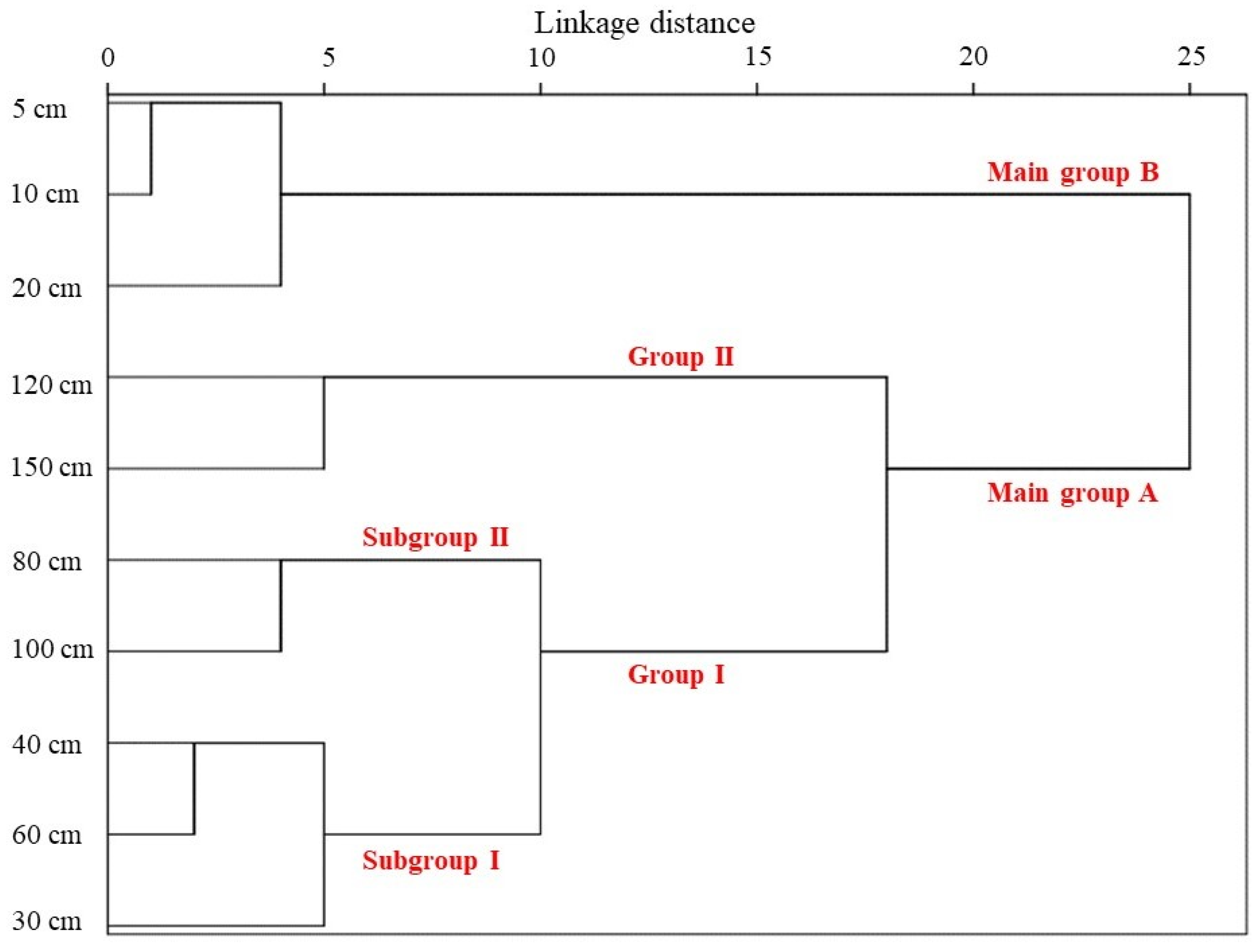
3.2. Determination of the Water Sources with Different Mixing Models

For the normal condition, MixSIR estimated a higher value of proportional contribution in the 0–20 cm depth, in comparison to MixSIAR and SIAR (Figure 5, p < 0.05). Nevertheless, the proportions in the other soil layers were similar among the three models (p > 0.05), except at the first, fourth, and fifth sampling periods. The specific mean proportion of RWU at different sampling times determined by MixSIAR was 49.7 ± 16.3%, 18.3 ± 6.9%, 16.6 ± 5.9% and 15.4 ± 6.8% in the 0–20 cm, 20–60 cm, 60–100 cm and 100–150 cm soil layers; 74.2 ± 19.5%, 8.5 ± 8.5%, 10.8 ± 10.5% and 6.5 ± 4.3% in the MixSIR; and 57.3 ± 16.0%, 17.4 ± 6.9%, 13.7 ± 6.2% and 11.5 ± 5.7% in the SIAR model, respectively. Accordingly, the three Bayesian mixing models indicated the 0–20 cm soil layer as the main RWU depth. Overall, the results suggested that there were significant differences (p < 0.05) in the proportional contributions of each soil layer in most sampling periods among three Bayesian models, while no significant difference (p > 0.05) was found in the main RWU depth among the mixing models under the normal condition.

According to Figure 5, under the wet condition, the proportion of the 0–20 cm layer estimated by the MixSIR was higher that of MixSIAR and SIAR (p < 0.05); with 91.4 ± 3.0%, 47.1 ± 6.5% and 28.8 ± 1.9% for the first sampling time, respectively. However, it was lower in other soil depths. The three models showed that the 0–20 cm soil layer was the main RWU depth at most sampling times. Nevertheless, the maximum contribution at fifth sampling time was derived from the 0–20 cm and 20–60 cm depth. In addition, the mean relative contributions of the seven sampling times were 57.3 ± 14.9%, 19.3 ± 12.7%, 12.4 ± 5.1% and 11.0 ± 3.8% in the 0–20 cm, 20–60 cm, 60–100 cm and 100–150 cm soil layers in the MixSIAR; 77.5 ± 19.8%, 13.9 ± 14.8%, 4.7 ± 3.6% and 12.0 ± 9.0% in the MixSIR; and 53.2 ± 14.8%, 21.4 ± 11.5%, 13.3 ± 7.1% and 12.0 ± 9.0% in the SIAR model, respectively.

For the dry condition, there were significant differences (p < 0.05) in the proportion in shallow layers (0–20 cm) and middle soil layers (20–60 cm) among the Bayesian models, except for individual sampling periods (Figure 5). The mean relative contributions at different sampling times were 39.2 ± 14.1%, 25.9 ± 5.4%, 18.4 ± 5.2% and 16.4 ± 4.4% in the 0–20 cm, 20–60 cm, 60–100 cm and 100–150 cm soil layers in the MixSIAR; 51.4 ± 24.6%, 20.4 ± 25.9%, 11.6 ± 7.1% and 16.6 ± 13.1% in the MixSIR; and 46.4 ± 14.9%, 25.0 ± 7.0%, 15.3 ± 4.7% and 13.2 ± 5.3% in the SIAR model, respectively. Collectively, these results suggested that the average proportion of the 0–20 cm layer under the dry condition was lower than that under the normal and wet conditions, indicating that wheat would decrease the RWU proportion of the 0–20 cm soil layer under the dry condition due to the less available soil water in shallow layers.

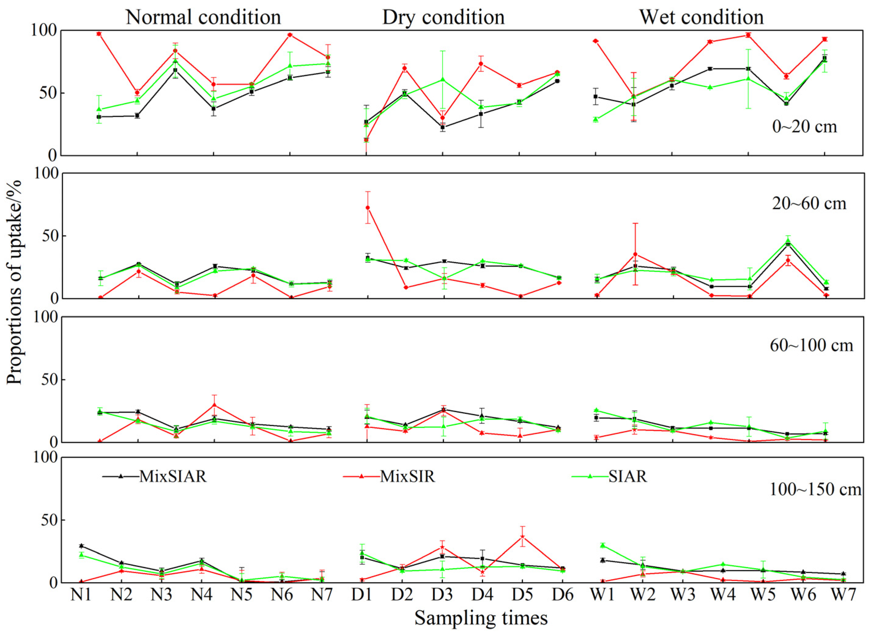
3.3. Performance of the Bayesian Mixing Models in Determining Water Source Proportion

Performances of the three mixing models in predicting water source proportion is shown in Figure 6. For the normal condition, the values of R², RMSE, IA and NS in different sampling times were 0.93, 0.25, 0.86 and 0.93 in the MixSIAR; 0.83, 0.77, 0.62 and 0.40 in the MixSIR; and 0.87, 0.45, 0.82 and 0.79 in the SIAR model, respectively. These results suggested that under the normal condition, the MixSIAR model performed better than the other two models. Under the dry condition, the MixSIR model had a larger value of R², IA, and NS and smaller value of RMSE than the SIAR and MixSIAR model, indicating that MixSIR was more reliable. Interestingly, the accuracy of the three mixing models decreased more under the wet condition than under the normal and dry condition, but the R² of MixSIAR (0.88) was still higher than other models (Figure 6). In total, the MixSIAR model had a larger value of R², IA and NS and a smaller value of RMSE than the MixSIR and SIAR, suggesting that MixSIAR exhibited relatively better performance for water source allocation, irrespective of the soil water condition.

4. Discussion

4.1. Evaluation of Water Source Apportionment within Three Bayesian Models

Analysis of RWU mechanisms (e.g., how roots grow and how they regulate hydraulic networks in response to environmental changes) is critical for modulating plant roots to facilitate water and nutrient uptake. Stable isotopes of oxygen and hydrogen (δ¹⁸O and δD) have been successfully applied to identify plant RWU, since the traditional methods have difficulties in quantifying the RWU temporally (irrigation, winter and summer precipitation, etc.) and spatially (shallow, middle and deep soil, groundwater, etc.) [8,39]. Recently, several mathematical models coupled with stable isotopes have been developed to estimate RWU [23,24,25]; however, these models (i.e., MixSIAR, MixSIR and SIAR) may neglect the differences among the methods for determining plant water source allocation. The model algorithms and soil moisture difference could be the factors causing the differences in determining the proportional contribution among the three mixing models.

A recent study suggested that the RWU proportions in the shallow layer estimated by the MixSIR model significantly differed from those in MixSIAR and SIAR, but there was no significant difference (p > 0.05) between SIAR and MixSIAR [32]. In this study, the average proportion of the 0–20 cm layer estimated by the three models appeared in the order of MixSIR > SIAR > MixSIAR under the normal and dry conditions, while the order was MixSIR > MixSIAR > SIAR under the wet condition. From the perspective of all sampling periods, there was no significant difference (p > 0.05) in the average proportions in the four layers as estimated by the three Bayesian models. Nevertheless, from the perspective of individual sampling time, there were significant differences in RWU proportions among the three mixing models (p < 0.05), except for the fifth and seventh sampling under the normal condition and the third sampling under the wet condition. Interestingly, although there were significant differences in the estimated proportional contributions of each soil layer among the three mixing models, the main RWU depth determined by the three Bayesian models showed no significant differences (p > 0.05), except for the third sampling under the dry condition and the sixth sampling under the wet condition. Our results showed that the different models lead to inconsistent or contradictory RWU results under the different SWC conditions. There are two comprehensive reasons that likely contributed to such differences. Firstly, the algorithm difference of the Bayesian models might cause the prediction difference among the three models; Secondly, the environment in which crops are grown, especially soil moisture, may also have affected the model’s prediction results [13,32]. Therefore, it is important to evaluate the performances of the models in order to identify the most suitable model for determining the RWU proportion.

Several studies reported that the MixSIAR and SIAR models exhibited similar performance and their performances were higher than that of MixSIR [32,40], while others indicated that the accuracy of MixSIR was better than that of SIAR [41] or MixSIAR [33] when SWC conditions were not considered. In this study, our results showed that, under the normal condition, the MixSIAR had a smaller RMSE and larger NS-value than MixSIR and SIAR (Figure 6), suggesting that MixSIAR had more reliable predictions. While the precision of MixSIAR and SIAR was reduced under normal conditions, the precision of MixSIR was improved under the dry condition. In particular, the NS-value of SIAR under the dry condition was negative (−0.20), indicating that the effectiveness of model performance was less reliable under this condition. After applying irrigation water of 90 mm, the difference between δD and δ¹⁸O of soil water in each layer was reduced, because water input eliminated the isotopic gradient distribution in the soil profile, which made it more difficult to determine crop water source partitioning. This may account for the reduced accuracy of these Bayesian models under the wet condition. Collectively, these results suggested that the performances of the three models in determining plant water source allocation varied with SWC conditions. Overall, the MixSIAR model showed better performance than the MixSIR and SIAR, regardless of the SWC (Figure 6).

Further, to confirm the above conclusion, two group data were added in order to verify the performance of the three models for determining plant water source allocation. One group of additional data from a previous study for the same site was used to demonstrate whether the MixSIAR model is better in water source division [9]. Here, two soil water conditions, i.e., normal and wet conditions, were considered, due to the fact that the sampling times were decreased under the dry condition, and the results showed that the input of irrigation water (wet condition) markedly decreased the accuracy of these mixing models. Figure 7a–f presents similar results; the ranking of the performances of the three models was MixSIAR, MixSIR and SIAR, respectively.

4.2. Implications for Water Source Partitions

The current results, as well as those from a previous study, recommend the MixSIAR model as the most appropriate for determining water source allocation, owing to its better performance than MixSIR and SIAR [42]. In addition, MixSIAR combined the advantages of these two models [27]. Furthermore, this work focused on the effects of soil water conditions on the model performance. Nevertheless, the simulation of MixSIAR in wet conditions was relatively poor, which might be attributed to the stable isotope overlap between potential water sources caused by water migration in the soil layer [43]. Hence, some prior information, for example, the relationships between root traits, soil moisture and nutrient availability, should be implemented to improve the model performance in RWU, especially under wet conditions [27,28,32,44].

The stable hydrogen and oxygen isotope analysis provides important grounds for determining the RWU proportion of each source for understanding the seasonal patterns of crop RWU in the agricultural water management. However, the focus on water transport from soil to plant might be too coarse, since soil water movement should pass through the cycle of the soil-plant-atmosphere continuum (SPAC). Therefore, detailed investigations are required to fill essential gaps in the water cycle system through a combination of other techniques and methods. For example, fertilizer application has great effects on water distribution in the soil and plant uptake, especially for water–fertilizer integration management [45]. Thus, more attention should be paid to the effects of the interactions between water and fertilizer uptake and their combination efficiency on RWU using carbon and nitrogen isotopes [46,47,48]. In addition, the outputs of RWU only presented a quantitative ratio of crop water use from each soil layer; the specific amount of root uptake is still unknown. Hence there is a need for the combination of stable isotopic methods and crop water requirements (ET) to convert the obtained percentages to water depth values according to the growth stage, which is useful for developing more efficient and rational schemes for farmers and water managers, particularly in arid and semi-arid regions [19,49,50]. Currently, the laser isotope spectrometry technique provides for continuous monitoring of water vapor isotopes with high resolution in the field to further understand RWU and evapotranspiration patterns [51,52]. Finally, few studies have focused on model analysis of RWU; for deeper understanding of the mechanism of soil water migration, more studies are needed to integrate the multi-objective isotope models, such as Simple Soil Plant Atmosphere Transfer (SISPAT), to explore the regularity of soil water and stable hydrogen and oxygen isotope transport [24].

5. Conclusions

In this study, the performances of three mixing models (MixSIAR, MixSIR, SIAR) for determining RWU under different soil water conditions were evaluated. The three Bayesian models reported significantly different values of water uptake proportions in most sampling periods (p < 0.05). Typically, the proportions within the 0–20 cm depth for MixSIR, MixSIAR and SIAR were 50.3%, 31.8% and 43.7% at the third sampling under the normal condition (p < 0.05), respectively. However, the main RWU depth estimated by the three Bayesian models showed no significant differences (p > 0.05), except for the third sampling under the dry condition and sixth sampling under the wet condition. Generally, the MixSIAR model had larger values of R², IA and NS and smaller values of RMSE than the MixSIR and SIAR models. Thus, according to the characteristics of the model itself and the results of the inter-comparison of tracer mixing models combined with the field data, the MixSIAR model is recommended for estimating plant water source allocation, regardless of the effects of soil water conditions.

References

1. Chang, E.; Li, P.; Li, Z.; Xiao, L.; Zhao, B.; Su, Y.; Feng, Z. Using water isotopes to analyze water uptake during vegetation succession on abandoned cropland on the Loess Plateau, China. Catena 2019, 181, 104095. [Google Scholar] [CrossRef]
2. Vargas, A.I.; Schaffer, B.; Li, Y.H.; Sternberg, L.D.L. Testing plant use of mobile vs immobile soil water sources using stable isotope experiments. New Phytol. 2017, 215, 582–594. [Google Scholar] [CrossRef] [PubMed] [Green Version]
3. Grossiord, C.; Sevanto, S.; Dawson, T.E.; Adams, H.D.; Collins, A.D.; Dickman, L.T.; Newman, B.D.; Stockton, E.A.; McDowell, N.G. Warming combined with more extreme precipitation regimes modifies the water sources used by trees. New Phytol. 2017, 213, 584–596. [Google Scholar] [CrossRef] [PubMed]
4. Liu, J.; Si, Z.; Li, S.; Kader Mounkaila Hamani, A.; Zhang, Y.; Wu, L.; Gao, Y.; Duan, A. Variations in water sources used by winter wheat across distinct rainfall years in the North China Plain. J. Hydrol. 2023, 618, 129186. [Google Scholar] [CrossRef]
5. Darouich, H.; Karfoul, R.; Ramos, T.B.; Moustafa, A.; Shaheen, B.; Pereira, L.S. Crop water requirements and crop coefficients for jute mallow (Corchorus olitorius L.) using the SIMDualKc model and assessing irrigation strategies for the Syrian Akkar region. Agric. Water Manag. 2021, 255, 107038. [Google Scholar] [CrossRef]
6. Gao, J.; Yang, X.; Zheng, B.; Liu, Z.; Zhao, J.; Sun, S.; Li, K.; Dong, C. Effects of climate change on the extension of the potential double cropping region and crop water requirements in Northern China. Agric. For. Meteorol. 2019, 268, 146–155. [Google Scholar] [CrossRef]
7. Gao, Y.; Yang, L.; Shen, X.; Li, X.; Sun, J.; Duan, A.; Wu, L. Winter wheat with subsurface drip irrigation (SDI): Crop coefficients, water-use estimates, and effects of SDI on grain yield and water use efficiency. Agric. Water Manag. 2014, 146, 1–10. [Google Scholar] [CrossRef]
8. Penna, D.; Geris, J.; Hopp, L.; Scandellari, F. Water sources for root water uptake: Using stable isotopes of hydrogen and oxygen as a research tool in agricultural and agroforestry systems. Agric. Ecosyst. Environ. 2020, 291, 106790. [Google Scholar] [CrossRef]
9. Liu, J.; Si, Z.; Wu, L.; Chen, J.; Gao, Y.; Duan, A. Using stable isotopes to quantify root water uptake under a new planting pattern of high-low seed beds cultivation in winter wheat. Soil Tillage Res. 2021, 205, 104816. [Google Scholar] [CrossRef]
10. Zhao, X.; Li, F.; Ai, Z.; Li, J.; Gu, C. Stable isotope evidences for identifying crop water uptake in a typical winter wheat-summer maize rotation field in the North China Plain. Sci. Total Environ. 2018, 618, 121–131. [Google Scholar] [CrossRef]
11. Ma, Y.; Song, X. Using stable isotopes to determine seasonal variations in water uptake of summer maize under different fertilization treatments. Sci. Total Environ. 2016, 550, 471–483. [Google Scholar] [CrossRef] [PubMed]
12. Liu, Z.; Jia, G.; Yu, X.; Lu, W.; Zhang, J. Water use by broadleaved tree species in response to changes in precipitation in a mountainous area of Beijing. Agric. Ecosyst. Environ. 2018, 251, 132–140. [Google Scholar] [CrossRef]
13. Stock, B.C.; Semmens, B.X. Unifying error structures in commonly used biotracer mixing models. Ecology 2016, 97, 2562–2569. [Google Scholar] [CrossRef] [PubMed]
14. Asbjornsen, H.; Mora, G.; Helmers, M.J. Variation in water uptake dynamics among contrasting agricultural and native plant communities in the Midwestern U.S. Agric. Ecosyst. Environ. 2007, 121, 343–356. [Google Scholar] [CrossRef]
15. Schwartz, N.; Carminati, A.; Javaux, M. The impact of mucilage on root water uptake—A numerical study. Water Resour. Res. 2016, 52, 264–277. [Google Scholar] [CrossRef] [Green Version]
16. Zhang, X.X.; Whalley, P.A.; Ashton, R.W.; Evans, J.; Hawkesford, M.J.; Griffiths, S.; Huang, Z.D.; Zhou, H.; Mooney, S.J.; Whalley, W.R. A comparison between water uptake and root length density in winter wheat: Effects of root density and rhizosphere properties. Plant Soil 2020, 451, 345–356. [Google Scholar] [CrossRef] [PubMed]
17. Li, N.; Yue, X. Calibrating the spatiotemporal root density distribution for macroscopic water uptake models using Tikhonov regularization. Water Resour. Res. 2018, 54, 1781–1795. [Google Scholar] [CrossRef]
18. Hoekstra, N.J.; Finn, J.A.; Hofer, D.; Lüscher, A. The effect of drought and interspecific interactions on depth of water uptake in deep- and shallow-rooting grassland species as determined by δ<sup>18</sup>O natural abundance. Biogeosciences 2014, 11, 4493–4506. [Google Scholar] [CrossRef] [Green Version]
19. Yang, B.; Wang, P.; You, D.; Liu, W. Coupling evapotranspiration partitioning with root water uptake to identify the water consumption characteristics of winter wheat: A case study in the North China Plain. Agric. For. Meteorol. 2018, 259, 296–304. [Google Scholar] [CrossRef]
20. Coelho, E.F.; Or, D. Root distribution and water uptake patterns of corn under surface and subsurface drip irrigation. Plant Soil 1999, 206, 123–136. [Google Scholar] [CrossRef]
21. Zhao, P.; Tang, X.; Zhao, P.; Tang, J. Dynamics of water uptake by maize on sloping farmland in a shallow Entisol in Southwest China. Catena 2016, 147, 511–521. [Google Scholar] [CrossRef]
22. Mora, G.; Jahren, A. Isotopic evidence for the role of plant development on transpiration in deciduous forests of southern United States. Glob. Biogeochem. Cycle 2003, 17, 11–13. [Google Scholar] [CrossRef]
23. Phillips, D.L.; Newsome, S.D.; Gregg, J.W. Combining sources in stable isotope mixing models: Alternative methods. Oecologia 2005, 144, 520–527. [Google Scholar] [CrossRef] [PubMed]
24. Rossatto, D.R.; de Carvalho Ramos Silva, L.; Villalobos-Vega, R.; Sternberg, L.d.S.L.; Franco, A.C. Depth of water uptake in woody plants relates to groundwater level and vegetation structure along a topographic gradient in a neotropical savanna. Environ. Exp. Bot. 2012, 77, 259–266. [Google Scholar] [CrossRef]
25. Stock, B.C.; Semmens, B.X.; Ward, E.J.; Moore, J.W.; Parnell, A.; Jackson, A.L.; Phillips, D.L.; Bearhop, S.; Inger, R. MixSIAR: Advanced stable isotope mixing models in R. In Proceedings of the ESA Convention, Sacramento Convention Center, Sacramento, CA, USA, 10–15 August 2014. [Google Scholar]
26. Parnell, A.C.; Inger, R.; Bearhop, S.; Jackson, A.L. Source Partitioning Using Stable Isotopes: Coping with Too Much Variation. PLoS ONE 2010, 5, e9672. [Google Scholar] [CrossRef]
27. Stock, B.; Jackson, A.; Ward, E.; Parnell, A.; Phillips, D.; Semmens, B. Analyzing mixing systems using a new generation of Bayesian tracer mixing models. PeerJ 2018, 6, e5096. [Google Scholar] [CrossRef]
28. Moore, J.W.; Semmens, B.X. Incorporating uncertainty and prior information into stable isotope mixing models. Ecol. Lett. 2008, 11, 470–480. [Google Scholar] [CrossRef]
29. Parnell, A.; Phillips, D.; Bearhop, S.; Semmens, B.; Ward, E.; Moore, J.; Jackson, A.; Grey, J.; Kelly, D.; Inger, R. Bayesian Stable Isotope Mixing Models. Environmetrics 2013, 24, 387–399. [Google Scholar] [CrossRef] [Green Version]
30. Rothfuss, Y.; Javaux, M. Reviews and syntheses: Isotopic approaches to quantify root water uptake: A review and comparison of methods. Biogeosciences 2017, 14, 2199–2224. [Google Scholar] [CrossRef] [Green Version]
31. Jackson, A.L.; Inger, R.; Bearhop, S.; Parnell, A. Erroneous behaviour of MixSIR, a recently published Bayesian isotope mixing model: A discussion of Moore and Semmens (2008). Ecol. Lett. 2008, 12, E1–E5. [Google Scholar] [CrossRef]
32. Wang, J.; Lu, N.; Fu, B. Inter-comparison of stable isotope mixing models for determining plant water source partitioning. Sci. Total Environ. 2019, 666, 685–693. [Google Scholar] [CrossRef]
33. Zhang, Y.; Zhang, M.; Wang, S.; Guo, R.; Che, C.; Du, Q.; Ma, Z.; Su, P. Comparison of different methods for determining plant water sources based on stable oxygen isotope. Chin. J. Ecol. 2020, 39, 1356–1368. [Google Scholar]
34. Evaristo, J.; Mcdonnell, J.J.; Clemens, J. Plant source water apportionment using stable isotopes: A comparison of simple linear, two-compartment mixing model approaches (revision 3). Hydrol. Process. 2017, 31, 3750–3758. [Google Scholar] [CrossRef]
35. Si, Z.; Zain, M.; Mehmood, F.; Wang, G.; Gao, Y.; Duan, A. Effects of nitrogen application rate and irrigation regime on growth, yield, and water-nitrogen use efficiency of drip-irrigated winter wheat in the North China Plain. Agric. Water Manag. 2020, 231, 106002. [Google Scholar] [CrossRef]
36. Qin, A.Z.; Ning, D.F.; Liu, Z.D.; Duan, A.W. Analysis of the Accuracy of an FDR Sensor in Soil Moisture Measurement under Laboratory and Field Conditions. J. Sens. 2021, 2021, 10. [Google Scholar] [CrossRef]
37. Donovan, L.A.; Ehleringer, J.R. Water Stress and Use of Summer Precipitation in a Great Basin Shrub Community. Funct. Ecol. 1994, 8, 289–297. [Google Scholar] [CrossRef]
38. Craig, H. Isotopic variation in meteoric waters. Science 1961, 133, 1702–1703. [Google Scholar] [CrossRef]
39. Pan, Y.-X.; Wang, X.-P.; Ma, X.-Z.; Zhang, Y.-F.; Hu, R. The stable isotopic composition variation characteristics of desert plants and water sources in an artificial revegetation ecosystem in Northwest China. Catena 2020, 189, 104499. [Google Scholar] [CrossRef]
40. Mabit, L.; Gibbs, M.; Mbaye, M.; Meusburger, K.; Toloza, A.; Resch, C.; Klik, A.; Swales, A.; Alewell, C. Novel application of Compound Specific Stable Isotope (CSSI) techniques to investigate on-site sediment origins across arable fields. Geoderma 2018, 316, 19–26. [Google Scholar] [CrossRef]
41. Brett, M.T. Resource polygon geometry predicts Bayesian stable isotope mixing model bias. Mar. Ecol. Prog. Ser. 2014, 514, 1–12. [Google Scholar] [CrossRef] [Green Version]
42. Ma, Y.; Song, X. Applying stable isotopes to determine seasonal variability in evapotranspiration partitioning of winter wheat for optimizing agricultural management practices. Sci. Total Environ. 2019, 654, 633–642. [Google Scholar] [CrossRef]
43. Meng, L.; Zhao, Z.; Lu, L.; Zhou, J.; Luo, D.; Fan, R.; Li, S.; Jiang, Q.; Huang, T.; Yang, H.; et al. Source identification of particulate organic carbon using stable isotopes and n-alkanes: Modeling and application. Water Res. 2021, 197, 117083. [Google Scholar] [CrossRef] [PubMed]
44. Corneo, P.E.; Kertesz, M.A.; Bakhshandeh, S.; Tahaei, H.; Barbour, M.M.; Dijkstra, F.A. Studying root water uptake of wheat genotypes in different soils using water δ18O stable isotopes. Agric. Ecosyst. Environ. 2018, 264, 119–129. [Google Scholar] [CrossRef]
45. Yan, F.; Zhang, F.; Fan, X.; Fan, J.; Wang, Y.; Zou, H.; Wang, H.; Li, G. Determining irrigation amount and fertilization rate to simultaneously optimize grain yield, grain nitrogen accumulation and economic benefit of drip-fertigated spring maize in northwest China. Agric. Water Manag. 2021, 243, 106440. [Google Scholar] [CrossRef]
46. Quan, Z.; Li, S.; Zhang, X.; Zhu, F.; Li, P.; Sheng, R.; Chen, X.; Zhang, L.-M.; He, J.-Z.; Wei, W.; et al. Fertilizer nitrogen use efficiency and fates in maize cropping systems across China: Field 15N tracer studies. Soil Tillage Res. 2020, 197, 104498. [Google Scholar] [CrossRef]
47. Rocha, K.F.; Mariano, E.; Grassmann, C.S.; Trivelin, P.C.O.; Rosolem, C.A. Fate of 15N fertilizer applied to maize in rotation with tropical forage grasses. Field Crops Res. 2019, 238, 35–44. [Google Scholar] [CrossRef]
48. El-Sharkawy, M.; Tafur, S. Genotypic and within canopy variation in leaf carbon isotope discrimination and its relation to short-term leaf gas exchange characteristics in cassava grown under rain-fed conditions in the tropics. Photosynthetica 2007, 45, 515–526. [Google Scholar] [CrossRef]
49. Ma, Y.; Song, X. Seasonal Variations in Water Uptake Patterns of Winter Wheat under Different Irrigation and Fertilization Treatments. Water 2018, 10, 1633. [Google Scholar] [CrossRef] [Green Version]
50. Wagle, P.; Skaggs, T.H.; Gowda, P.H.; Northup, B.K.; Neel, J.P.S. Flux variance similarity-based partitioning of evapotranspiration over a rainfed alfalfa field using high frequency eddy covariance data. Agric. For. Meteorol. 2020, 285-286, 107907. [Google Scholar] [CrossRef]
51. Yuan, Y.; Yuan, Y.; Du, T.; Wang, H.; Wang, L. Novel Keeling-plot-based methods to estimate the isotopic composition of ambient water vapor. Hydrol. Earth Syst. Sci. 2020, 24, 4491–4501. [Google Scholar] [CrossRef]
52. Aouade, G.; Ezzahar, J.; Amenzou, N.; Er-Raki, S.; Benkaddour, A.; Khabba, S.; Jarlan, L. Combining stable isotopes, Eddy Covariance system and meteorological measurements for partitioning evapotranspiration, of winter wheat, into soil evaporation and plant transpiration in a semi-arid region. Agric. Water Manag. 2016, 177, 181–192. [Google Scholar] [CrossRef]
Figure 1. Variations in precipitation and temperature during the experiment period. The downward arrows represent irrigation. The squares represent the sampling dates under different soil water content conditions: wet (black), dry (red) and normal (blue).
Agronomy 13 00843 g001
Figure 2. Variations of gravimetric soil water content (VSWC) in different soil layers under the normal, dry and wet conditions.
Agronomy 13 00843 g002
Figure 3. Hierarchical cluster analysis diagram of the soil water content.
Agronomy 13 00843 g003
Figure 4. δD-δ18O relationships for the water samples, local meteoric water line (LMWL) and soil water evaporation line (SWL).
Agronomy 13 00843 g004
Figure 5. Mean water-absorbing proportional contributions of wheat from each soil depth interval under various SWC conditions using MixSIAR (black line), MixSIR (red line) and SIAR (green line) models.
Agronomy 13 00843 g005
Figure 6. Mixing model performance indicators in water source partitioning under the normal, dry, and wet conditions and their combination (total).
Agronomy 13 00843 g006
Figure 7. Comparisons between predicted and observed value of δ18O in 2017–2018 (ac) and 2018–2019 (df) wheat seasons. The data originated from our previous study at the same site [9].
Agronomy 13 00843 g007