

Time Series Feature Extraction Using Transfer Learning Technology for Crop Pest Prediction


Abstract
:1. Introduction
2. Related Work
3. Time Series Feature Extraction Using a Transfer Learning Technology Method
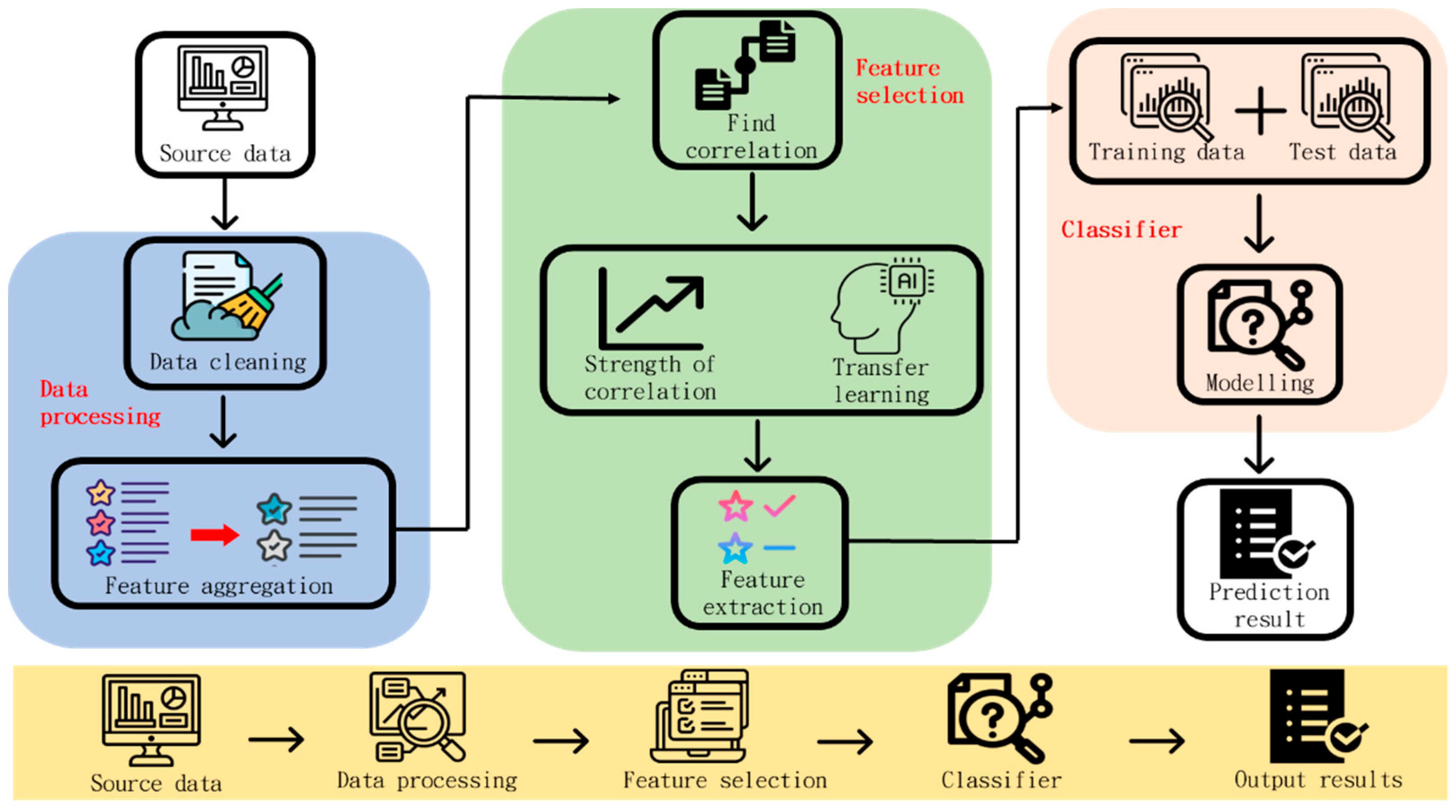
3.1. Overview of the Proposed System
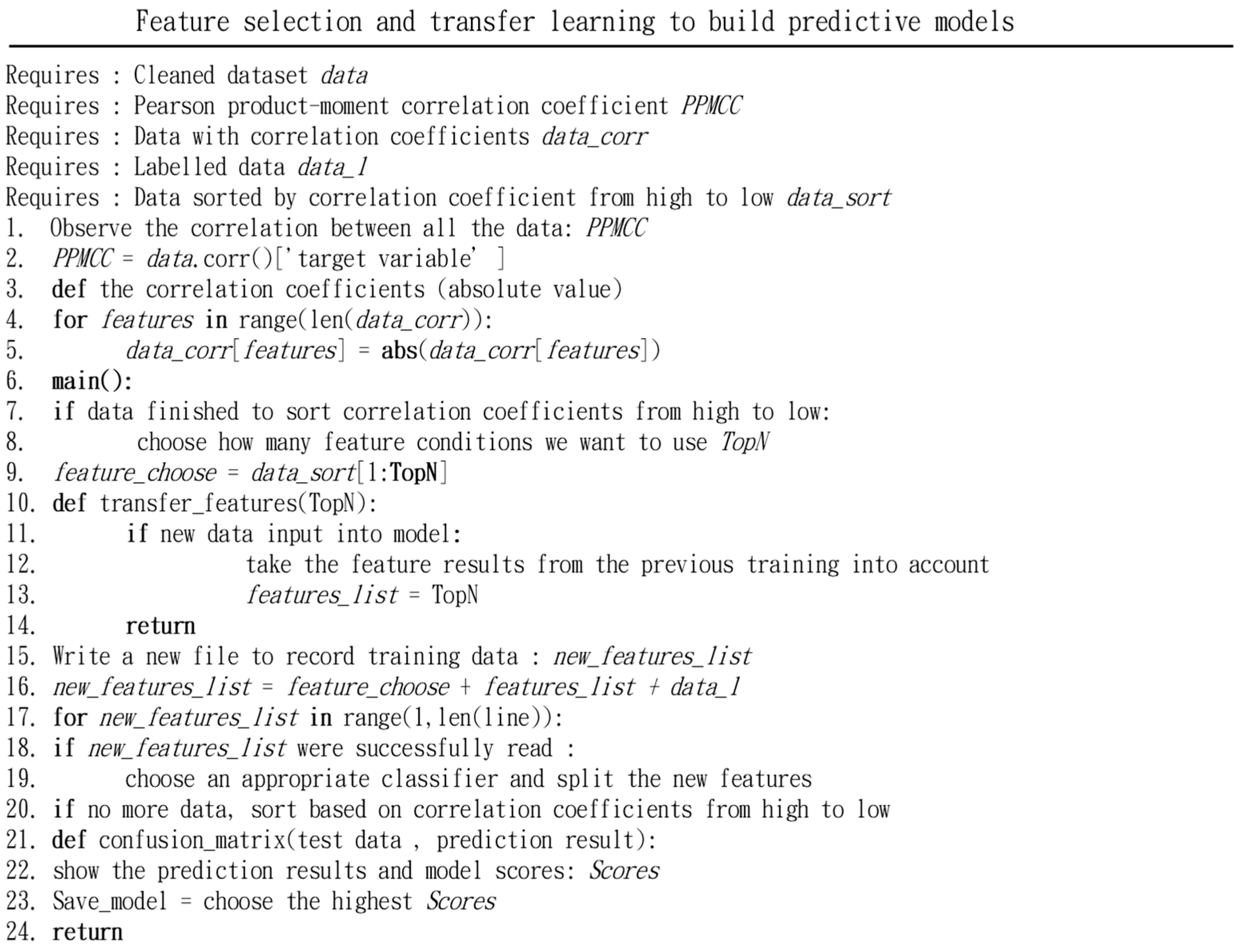
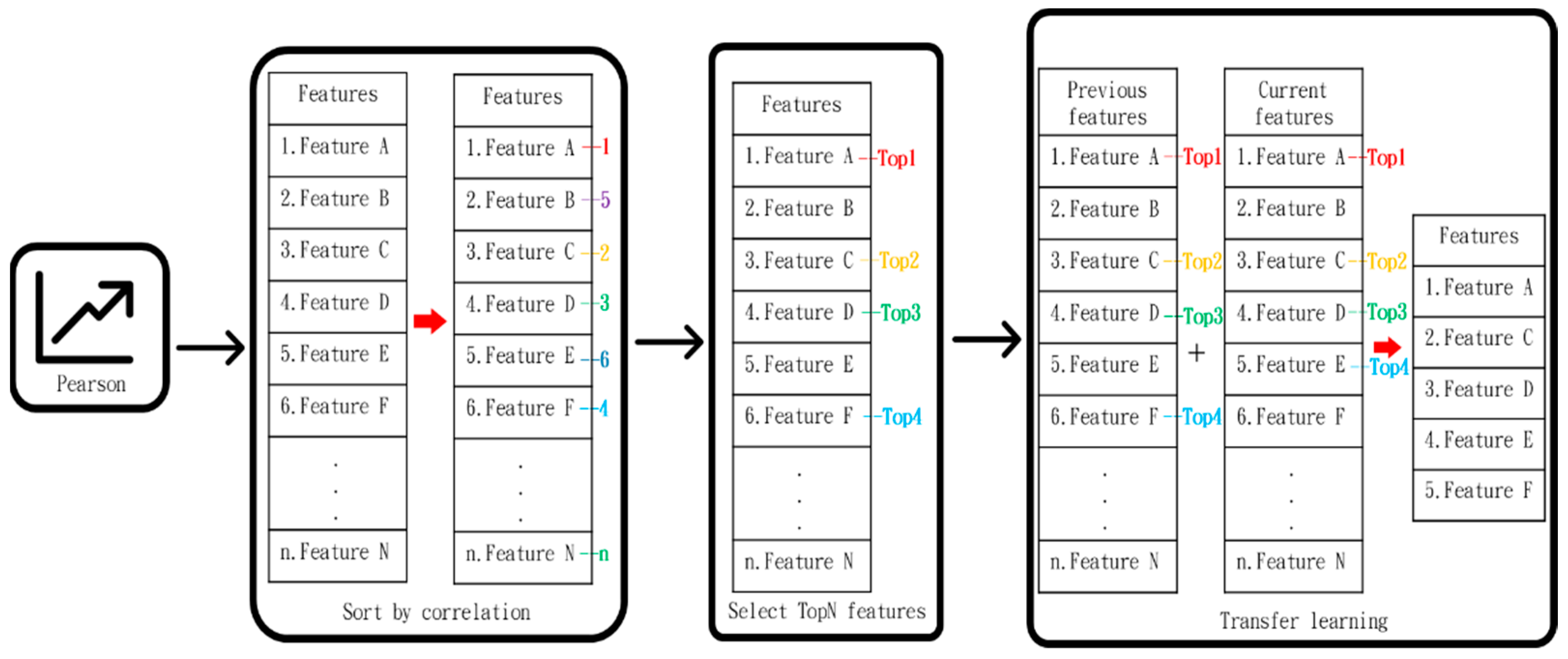
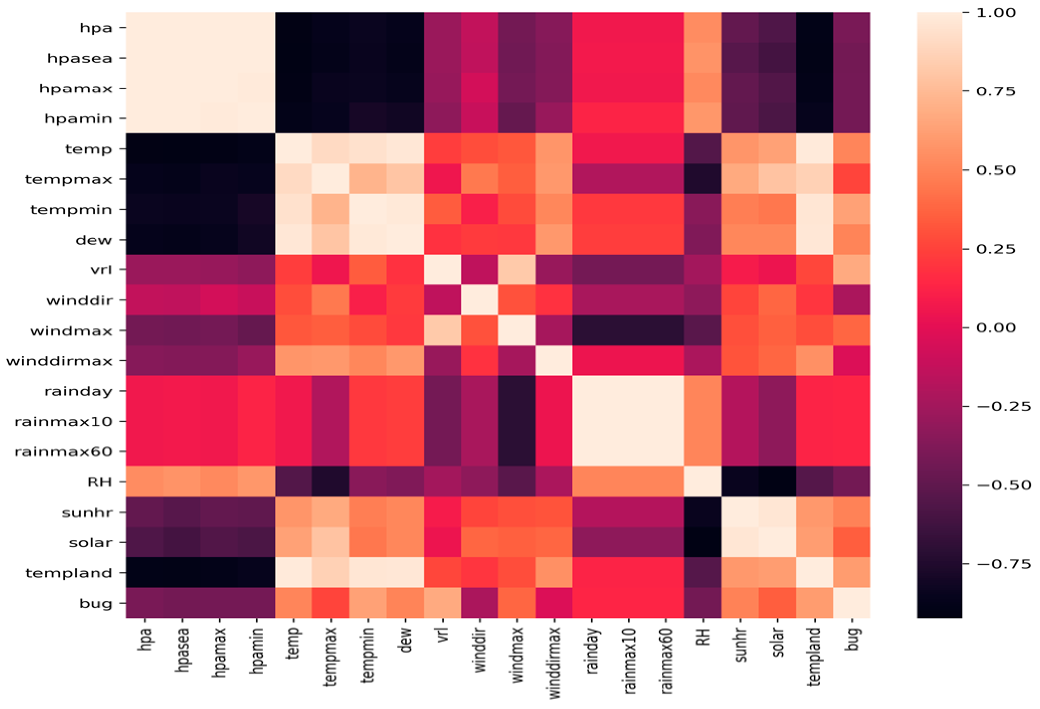
3.2. Design of the Recognition Model
3.3. Examples of Recognition Models
3.4. Performance Assessment
4. Experiments and Results
4.1. Prediction of Bactrocera Dorsalis Crop Pests
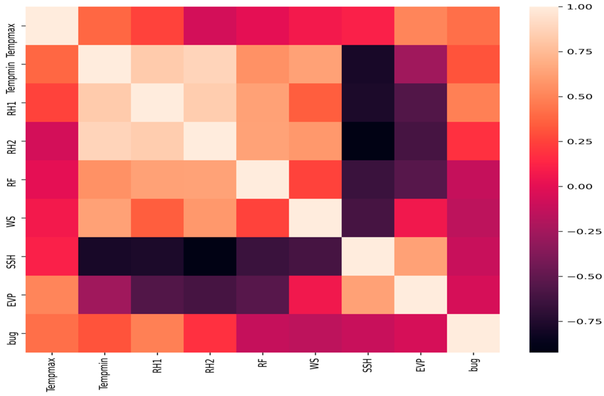
4.2. Prediction of Whitefly Crop Pests
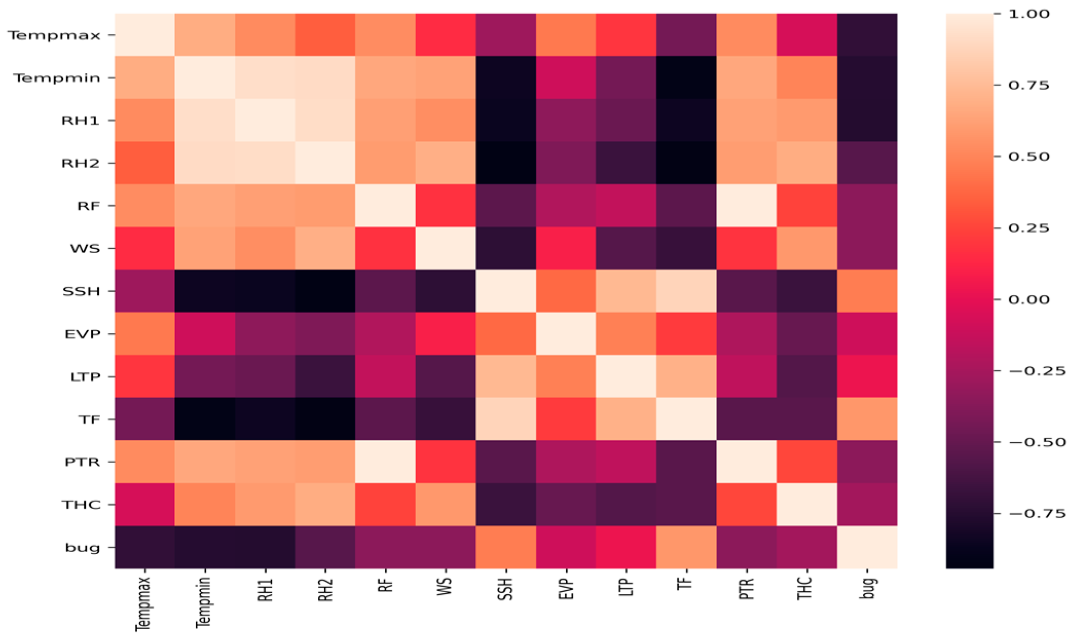
4.3. Prediction of Aphid Crop Pests
5. Conclusions
Author Contributions
Funding
Institutional Review Board Statement
Informed Consent Statement
Data Availability Statement
Conflicts of Interest
References
- Uddin, S.; Khan, A.; Hossain, E.; Moni, M.A. Comparing different supervised machine learning algorithms for disease prediction. BMC Med. Inform. Decis. Mak. 2019, 19, 1–16. [Google Scholar] [CrossRef]
- Krittanawong, C.; Virk, H.U.H.; Bangalore, S.; Wang, Z.; Johnson, K.W.; Pinotti, R.; Zhang, H.; Kaplin, S.; Narasimhan, B.; Kitai, T.; et al. Machine learning prediction in cardiovascular diseases: A meta-analysis. Sci. Rep. 2020, 10, 16057. [Google Scholar] [CrossRef] [PubMed]
- Chandrashekar, G.; Sahin, F. A survey on feature selection methods. Comput. Electr. Eng. 2014, 40, 16–28. [Google Scholar] [CrossRef]
- Khalid, S.; Khalil, T.; Nasreen, S. A survey of feature selection and feature extraction techniques in machine learning. In Proceedings of the Science and Information Conference (SAI), London, UK, 27–29 August 2014; pp. 372–378. [Google Scholar]
- Xue, B.; Zhang, M.; Browne, W.N.; Yao, X. A Survey on Evolutionary Computation Approaches to Feature Selection. IEEE Trans. Evol. Comput. 2015, 20, 606–626. [Google Scholar] [CrossRef] [Green Version]
- Cai, J.; Luo, J.; Wang, S.; Yang, S. Feature selection in machine learning: A new perspective. Neurocomputing 2018, 300, 70–79. [Google Scholar] [CrossRef]
- Salcedo-Sanz, S.; Cornejo-Bueno, L.; Prieto, L.; Paredes, D.; García-Herrera, R. Feature selection in machine learning prediction systems for renewable energy applications. Renew. Sustain. Energy Rev. 2018, 90, 728–741. [Google Scholar] [CrossRef]
- Tsai, M.-F.; Chu, Y.-C.; Li, M.-H.; Chen, L.-W. Smart Machinery Monitoring System with Reduced Information Transmission and Fault Prediction Methods Using Industrial Internet of Things. Mathematics 2021, 9, 3. [Google Scholar] [CrossRef]
- Masoudi-Sobhanzadeh, Y.; MotieGhader, H.; Masoudi-Nejad, A. FeatureSelect: A software for feature selection based on machine learning approaches. BMC Bioinform. 2019, 20, 1–17. [Google Scholar] [CrossRef]
- Christ, M.; Braun, N.; Neuffer, J.; Kempa-Liehr, A.W. Time Series FeatuRe Extraction on basis of Scalable Hypothesis tests (tsfresh—A Python package). Neurocomputing 2018, 307, 72–77. [Google Scholar] [CrossRef]
- Zhuang, F.; Qi, Z.; Duan, K.; Xi, D.; Zhu, Y.; Zhu, H.; Xiong, H.; He, Q. A Comprehensive Survey on Transfer Learning. Proc. IEEE 2021, 109, 43–76. [Google Scholar] [CrossRef]
- Shaha, M.; Pawar, M. Transfer learning for image classification. In Proceedings of the IEEE International Conference on Electronics, 2018 Second International Conference on Electronics, Communication and Aerospace Technology (ICECA 2018), Coimbatore, India, 29–31 March 2018; RVS Technical Campus: Coimbatore, India, 2018; pp. 656–660. [Google Scholar]
- Tan, C.; Sun, F.; Kong, T.; Zhang, W.; Yang, C.; Liu, C. A survey on deep transfer learning. In Proceedings of the International Conference on Artificial Neural Networks, Rhodes, Greece, 4–7 October 2018; pp. 270–277. Available online: https://link.springer.com/chapter/10.1007/978-3-030-01424-7_27 (accessed on 6 February 2023).
- Shen, F.; Chen, C.; Yan, R.; Gao, R.X. Bearing fault diagnosis based on SVD feature extraction and transfer learning classification. In Proceedings of the 2015 Prognostics and System Health Management Conference (PHM), Beijing, China, 21–23 October 2015; pp. 1–6. [Google Scholar]
- Newton, A.C.; Johnson, S.; Gregory, P. Implications of climate change for diseases, crop yields and food security. Euphytica 2011, 179, 3–18. [Google Scholar] [CrossRef]
- Sharma, A.; Jain, A.; Gupta, P.; Chowdary, V. Machine Learning Applications for Precision Agriculture: A Comprehensive Review. IEEE Access 2021, 9, 4843–4873. [Google Scholar] [CrossRef]
- Xie, C.; Wang, R.; Zhang, J.; Chen, P.; Dong, W.; Li, R.; Chen, T.; Chen, H. Multi-level learning features for automatic classification of field crop pests. Comput. Electron. Agric. 2018, 152, 233–241. [Google Scholar] [CrossRef]
- Xiao, Q.; Li, W.; Kai, Y.; Chen, P.; Zhang, J.; Wang, B. Occurrence prediction of pests and diseases in cotton on the basis of weather factors by long short term memory network. BMC Bioinform. 2019, 20, 688. [Google Scholar] [CrossRef] [PubMed]
- Chen, P.; Xiao, Q.; Zhang, J.; Xie, C.; Wang, B. Occurrence prediction of cotton pests and diseases by bidirectional long short-term memory networks with climate and atmosphere circulation. Comput. Electron. Agric. 2020, 176, 105612. [Google Scholar] [CrossRef]
- Senan, E.M.; Abunadi, I.; Jadhav, M.E.; Fati, S.M. Score and Correlation Coefficient-Based Feature Selection for Predicting Heart Failure Diagnosis by Using Machine Learning Algorithms. Comput. Math. Methods Med. 2021, 2021, 8500314. [Google Scholar] [CrossRef]
- Marouf, A.; Hasan, M.; Mahmud, H. Comparative analysis of feature selection algorithms for computational personality prediction from social media. IEEE Trans. Comput. Soc. Syst. 2020, 7, 587–599. [Google Scholar] [CrossRef]
- Marković, D.; Vujičić, D.; Tanasković, S.; Đorđević, B.; Ranđić, S.; Stamenković, Z. Prediction of Pest Insect Appearance Using Sensors and Machine Learning. Sensors 2021, 21, 4846. [Google Scholar] [CrossRef]
- Patil, R.R.; Kumar, S. Rice-Fusion: A Multimodality Data Fusion Framework for Rice Disease Diagnosis. IEEE Access 2022, 10, 5207–5222. [Google Scholar] [CrossRef]
- Bereciartua-Pérez, A.; Gómez, L.; Picón, A.; Navarra-Mestre, R.; Klukas, C.; Eggers, T. Insect counting through deep learning-based density maps estimation. Comput. Electron. Agric. 2022, 197, 106933. [Google Scholar] [CrossRef]
- Domingues, T.; Brandão, T.; Ferreira, J.C. Machine Learning for Detection and Prediction of Crop Diseases and Pests: A Comprehensive Survey. Agriculture 2022, 12, 1350. [Google Scholar] [CrossRef]


| Climate Characteristics | |
|---|---|
| 1. Mean pressure (hpa) | 13. Maximum gust wind direction (winddirmax) |
| 2. Mean sea-level pressure (hpasea) | 14. Cumulative rainfall (rainday) |
| 3. Maximum pressure (hpamax) | 15. Maximum precipitation (10 min) (rainmax10) |
| 4. Minimum pressure (hpamin) | 16. Maximum precipitation (60 min) (rainmax60) |
| 5. Mean temperature (temp) | 17. Accumulative irradiation time (sunhr) |
| 6. Maximum temperature (tempmax) | 18. Cumulative solar radiation (solar) |
| 7. Minimum temperature (tempmin) | 19. Mean ground temperature (0 cm) (templand) |
| 8. Dew point temperature (dew) | 20. Mean ground temperature (5 cm) (templand) |
| 9. Mean relative humidity (RH) | 21. Mean ground temperature (10 cm) (templand) |
| 10. Mean wind speed (vrl) | 22. Mean ground temperature (20 cm) (templand) |
| 11. Mean wind direction (winddir) | 23. Mean ground temperature (50 cm) (templand) |
| 12. Gust peak speed (windmax) | 24. Mean ground temperature (100 cm) (templand) |
| Number of Pests | Category |
|---|---|
| 0~10 | 0 |
| 10~20 | 1 |
| 20~30 | 2 |
| 30~50 | 3 |
| 50~100 | 4 |
| 100~200 | 5 |
| 200~500 | 6 |
| 500 or more | 7 |
| 2021 | KNN with Proposed Method | Random Forest with Proposed Method | SVM with Proposed Method | Naive Bayes with Proposed Method |
|---|---|---|---|---|
| ACC | 0.9196 | 0.9700 | 0.9700 | 0.9112 |
| Precision | 0.9396 | 0.9805 | 0.9800 | 0.9364 |
| Recall | 0.9392 | 0.9803 | 0.9803 | 0.9330 |
| F1-score | 0.9280 | 0.9772 | 0.9700 | 0.9250 |
| 2022 | KNN with Proposed Method | Random Forest with Proposed Method | SVM with Proposed Method | Naive Bayes with Proposed Method |
|---|---|---|---|---|
| ACC | 1.0000 | 1.0000 | 1.0000 | 1.0000 |
| Precision | 1.0000 | 1.0000 | 1.0000 | 1.0000 |
| Recall | 1.0000 | 1.0000 | 1.0000 | 1.0000 |
| F1-score | 1.0000 | 1.0000 | 1.0000 | 1.0000 |
| 2021 | KNN | Random Forest | SVM | Naive Bayes |
|---|---|---|---|---|
| ACC | 0.7300 | 0.88 | 0.881 | 0.88 |
| Precision | 0.6892 | 0.9565 | 0.85 | 0.9555 |
| Recall | 0.8380 | 0.9142 | 0.9143 | 0.9142 |
| F1-score | 0.6954 | 0.9204 | 0.9200 | 0.9200 |
| 2022 | KNN | Random Forest | SVM | Naive Bayes |
|---|---|---|---|---|
| ACC | 0.8055 | 0.8050 | 0.8055 | 0.8000 |
| Precision | 0.7666 | 0.9247 | 0.7666 | 0.9247 |
| Recall | 0.7407 | 0.7410 | 0.7400 | 0.7407 |
| F1-score | 0.6083 | 0.7454 | 0.6080 | 0.7450 |
| Climate Characteristics |
|---|
|
| Whitefly | KNN with Proposed Method | Random Forest with Proposed Method | SVM with Proposed Method | Naive Bayes with Proposed Method | Related Work [18] |
|---|---|---|---|---|---|
| ACC | 0.95555 | 0.94444 | 0.84444 | 0.7888 | 0.9244 |
| F1-score | 0.95553 | 0.94438 | 0.84413 | 0.7886 | 0.9243 |
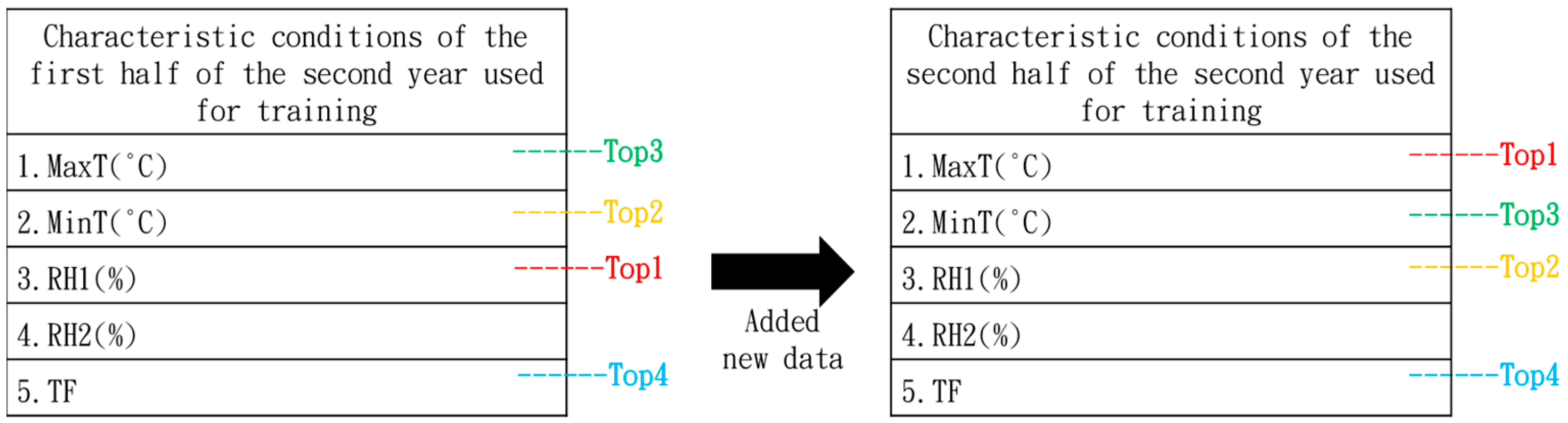
| Climate Characteristics | |
|---|---|
| 1. MaxT (°C) | 7. SSH (h) |
| 2. MinT (°C) | 8. EVP (mm) |
| 3. RH1 (%) | 9. LTP |
| 4. RH2 (%) | 10. TF |
| 5. RF (mm) | 11. PTR |
| 6. WS (kmph) | 12. THC |
| Aphid | KNN with Proposed Method | Random Forest with Proposed Method | SVM with Proposed Method | Naive Bayes with Proposed Method | Related Work [19] |
|---|---|---|---|---|---|
| ACC | 0.8898 | 0.9661 | 0.8983 | 0.8305 | 0.8298 |
| F1-score | 0.8959 | 0.9725 | 0.9048 | 0.8430 | 0.8234 |
Disclaimer/Publisher’s Note: The statements, opinions and data contained in all publications are solely those of the individual author(s) and contributor(s) and not of MDPI and/or the editor(s). MDPI and/or the editor(s) disclaim responsibility for any injury to people or property resulting from any ideas, methods, instructions or products referred to in the content. |
© 2023 by the authors. Licensee MDPI, Basel, Switzerland. This article is an open access article distributed under the terms and conditions of the Creative Commons Attribution (CC BY) license (https://creativecommons.org/licenses/by/4.0/).
Share and Cite
Tsai, M.-F.; Lan, C.-Y.; Wang, N.-C.; Chen, L.-W. Time Series Feature Extraction Using Transfer Learning Technology for Crop Pest Prediction. Agronomy 2023, 13, 792. https://doi.org/10.3390/agronomy13030792
Tsai M-F, Lan C-Y, Wang N-C, Chen L-W. Time Series Feature Extraction Using Transfer Learning Technology for Crop Pest Prediction. Agronomy. 2023; 13(3):792. https://doi.org/10.3390/agronomy13030792
Chicago/Turabian StyleTsai, Ming-Fong, Chun-Ying Lan, Neng-Chung Wang, and Lien-Wu Chen. 2023. "Time Series Feature Extraction Using Transfer Learning Technology for Crop Pest Prediction" Agronomy 13, no. 3: 792. https://doi.org/10.3390/agronomy13030792