
Wheat Yield Gap Assessment in Using the Comparative Performance Analysis (CPA)
 ,
,  , ,
, ,
Abstract
:1. Introduction
2. Materials and Methods
3. Results
3.1. Production Process Documentation
3.2. Estimating Yield Gap Using the CPA Method
3.3. The Range of CPA Approach Variables and Their Correlation
3.4. Wheat Yield Limiting Factors and Yield Gap Prediction
4. Discussion
5. Conclusions
Author Contributions
Funding
Institutional Review Board Statement
Informed Consent Statement
Data Availability Statement
Acknowledgments
Conflicts of Interest
References
- Fedoroff, N.V. Food in a Future of 10 Billion. Agric. Food Secur. 2015, 4, 11. [Google Scholar] [CrossRef] [Green Version]
- Gerland, P.; Raftery, A.E.; Ševčíková, H.; Li, N.; Gu, D.; Spoorenberg, T.; Alkema, L.; Fosdick, B.K.; Chunn, J.; Lalic, N.; et al. World Population Stabilization Unlikely This Century. Science 2014, 346, 234–237. [Google Scholar] [CrossRef] [Green Version]
- Guilpart, N.; Grassini, P.; Sadras, V.O.; Timsina, J.; Cassman, K.G. Estimating Yield Gaps at the Cropping System Level. Field Crops Res. 2017, 206, 21–32. [Google Scholar] [CrossRef]
- Cassman, K.G. What Do We Need to Know about Global Food Security? Glob. Food Sec. 2012, 1, 81–82. [Google Scholar] [CrossRef]
- Chapagain, T.; Good, A. Yield and Production Gaps in Rainfed Wheat, Barley, and Canola in Alberta. Front. Plant Sci. 2015, 6, 990. [Google Scholar] [CrossRef] [Green Version]
- Soltani, A.; Hajjarpour, A.; Vadez, V. Analysis of Chickpea Yield Gap and Water-Limited Potential Yield in Iran. Field Crops Res. 2016, 185, 21–30. [Google Scholar] [CrossRef]
- Soltani, A.; Alimagham, S.M.; Nehbandani, A.; Torabi, B.; Zeinali, E.; Zand, E.; Ghassemi, S.; Vadez, V.; Sinclair, T.R.; van Ittersum, M.K. Modeling Plant Production at Country Level as Affected by Availability and Productivity of Land and Water. Agric. Syst. 2020, 183, 102859. [Google Scholar] [CrossRef]
- The State of Food Security and Nutrition in the World 2022; Food and Agriculture Organization of the United Nations: Rome, Italy, 2022. [CrossRef]
- Gaydon, D.S.; Balwinder-Singh; Wang, E.; Poulton, P.L.; Ahmad, B.; Ahmed, F.; Akhter, S.; Ali, I.; Amarasingha, R.; Chaki, A.K.; et al. Evaluation of the APSIM Model in Cropping Systems of Asia. Field Crops Res. 2017, 204, 52–75. [Google Scholar] [CrossRef]
- Anderson, W.; Johansen, C.; Siddique, K.H.M. Addressing the Yield Gap in Rainfed Crops: A Review. Agron. Sustain. Dev. 2016, 36, 18. [Google Scholar] [CrossRef] [Green Version]
- Espe, M.; Cassman, K.; Yang, H.; Guilpart, N.; Grassini, P.; Van Wart, J.; Anders, M.; Beighley, D.; Harrell, D.; Linscombe, S.; et al. Yield Gap Analysis of US Rice Production Systems Shows Opportunities for Improvement. Field Crops Res. 2016, 196, 276–283. [Google Scholar] [CrossRef] [Green Version]
- Beza, E.; Silva, J.V.; Kooistra, L.; Reidsma, P. Review of Yield Gap Explaining Factors and Opportunities for Alternative Data Collection Approaches. Eur. J. Agron. 2017, 82, 206–222. [Google Scholar] [CrossRef]
- Zhang, S.Y.; Zhang, X.H.; Qiu, X.L.; Tang, L.; Zhu, Y.; Cao, W.X.; Liu, L.L. Quantifying the Spatial Variation in the Potential Productivity and Yield Gap of Winter Wheat in China. J. Integr. Agric. 2017, 16, 845–857. [Google Scholar] [CrossRef] [Green Version]
- Silva, J.V.; Reidsma, P.; Laborte, A.G.; van Ittersum, M.K. Explaining Rice Yields and Yield Gaps in Central Luzon, Philippines: An Application of Stochastic Frontier Analysis and Crop Modelling. Eur. J. Agron. 2017, 82, 223–241. [Google Scholar] [CrossRef]
- Van Ittersum, M.K.; Cassman, K.G.; Grassini, P.; Wolf, J.; Tittonell, P.; Hochman, Z. Yield Gap Analysis with Local to Global Relevance—A Review. F. Crop. Res. 2013, 143, 4–17. [Google Scholar] [CrossRef] [Green Version]
- Fischer, R.A. Definitions and Determination of Crop Yield, Yield Gaps, and of Rates of Change. Field Crops Res. 2015, 182, 9–18. [Google Scholar] [CrossRef]
- Lobell, D.B.; Cassman, K.G.; Field, C.B. Crop Yield Gaps: Their Importance, Magnitudes, and Causes. Annu. Rev. Environ. Resour. 2009, 34, 179–204. [Google Scholar] [CrossRef] [Green Version]
- Van Wart, J.; Kersebaum, K.C.; Peng, S.; Milner, M.; Cassman, K.G. Estimating Crop Yield Potential at Regional to National Scales. Field Crops Res. 2013, 143, 34–43. [Google Scholar] [CrossRef] [Green Version]
- De Bie, C.A.J.M. Comparative Performance Analysis of Agro-Ecosystems. ITC Dissertation. 2000. Available online: https://edepot.wur.nl/121245 (accessed on 21 December 2022).
- Hajjarpoor, A.; Soltani, A.; Zeinali, E.; Kashiri, H.; Aynehband, A.; Vadez, V. Using Boundary Line Analysis to Assess the On-Farm Crop Yield Gap of Wheat. Field Crops Res. 2018, 225, 64–73. [Google Scholar] [CrossRef]
- Gorjizad, A.; Dastan, S.; Soltani, A.; Ajam Norouzi, H. Large Scale Assessment of the Production Process and Rice Yield Gap Analysis by Comparative Performance Analysis and Boundary-Line Analysis Methods. Ital. J. Agron. 2019, 14, 123–131. [Google Scholar] [CrossRef] [Green Version]
- Nezamzade, E.; Soltani, E.N.Z.; Soltani, A.; Dastan, S.; Ajamnoroozi, H.A.N. Factors Causing Yield Gap in Rape Seed Production in the Eastern of Mazandaran Province, Iran. Ital. J. Agron. 2020, 15, 10–19. [Google Scholar] [CrossRef]
- Dehkordi, P.A.; Nehbandani, A.; Hassanpour-bourkheili, S.; Kamkar, B. Yield Gap Analysis Using Remote Sensing and Modelling Approaches: Wheat in the Northwest of Iran. Int. J. Plant Prod. 2020, 14, 443–452. [Google Scholar] [CrossRef]
- Casanova, D.; Goudriaan, J.; Bouma, J.; Epema, G.F. Yield Gap Analysis in Relation to Soil Properties in Direct-Seeded Flooded Rice. Geoderma 1999, 91, 191–216. [Google Scholar] [CrossRef]
- Kitchen, N.R.; Drummond, S.T.; Lund, E.D.; Sudduth, K.A.; Buchleiter, G.W. Soil Electrical Conductivity and Topography Related to Yield for Three Contrasting Soil–Crop Systems. Agron. J. 2003, 95, 483–495. [Google Scholar] [CrossRef]
- Shatar, T.M.; Mcbratney, A.B. Boundary-Line Analysis of Field-Scale Yield Response to Soil Properties. J. Agric. Sci. 2004, 142, 553–560. [Google Scholar] [CrossRef]
- Tittonell, P.; Shepherd, K.D.; Vanlauwe, B.; Giller, K.E. Unravelling the Effects of Soil and Crop Management on Maize Productivity in Smallholder Agricultural Systems of Western Kenya—An Application of Classification and Regression Tree Analysis. Agric. Ecosyst. Environ. 2008, 123, 137–150. [Google Scholar] [CrossRef] [Green Version]
- Tittonell, P.; Giller, K.E. When Yield Gaps Are Poverty Traps: The Paradigm of Ecological Intensification in African Smallholder Agriculture. Field Crops Res. 2013, 143, 76–90. [Google Scholar] [CrossRef] [Green Version]
- Huang, X.; Wang, L.; Yang, L.; Kravchenko, A.N. Management Effects on Relationships of Crop Yields with Topography Represented by Wetness Index and Precipitation. Agron. J. 2008, 100, 1463–1471. [Google Scholar] [CrossRef] [Green Version]
- Tasistro, A. Use of Boundary Lines in Field Diagnosis and Research for Mexican Farmers. Better Crops Plant Food 2012, 96, 11–13. [Google Scholar]
- Grassini, P.; Hall, A.J.; Mercau, J.L. Benchmarking Sunflower Water Productivity in Semiarid Environments. Field Crops Res. 2009, 110, 251–262. [Google Scholar] [CrossRef]
- Menendez, F.J.; Satorre, E.H. Evaluating Wheat Yield Potential Determination in the Argentine Pampas. Agric. Syst. 2007, 95, 1–10. [Google Scholar] [CrossRef]
- Abeledo, L.G.; Savin, R.; Slafer, G.A. Wheat Productivity in the Mediterranean Ebro Valley: Analyzing the Gap between Attainable and Potential Yield with a Simulation Model. Eur. J. Agron. 2008, 4, 541–550. [Google Scholar] [CrossRef]
- Lu, C.; Fan, L. Winter Wheat Yield Potentials and Yield Gaps in the North China Plain. Field Crops Res. 2013, 143, 98–105. [Google Scholar] [CrossRef] [Green Version]
- Pradhan, R. The Effect of Land and Management Aspects on Maize Yield; International Institute for Geo-Information Science and Earth Observation: Enschede, The Netherlands, 2004. [Google Scholar]
- Barthold, V.V.; Soucek, S. An Historical Geography of Iran; Princeton University Press: Princeton, NJ, USA, 2014; 309p. [Google Scholar]
- Mclean, E.O. Soil PH and Lime Requirement. Methods Soil Anal. Part 2 Chem. Microbiol. Prop. 2015, 9, 199–224. [Google Scholar] [CrossRef]
- Nelson, D.W.; Sommers, L.E. Total Carbon, Organic Carbon, and Organic Matter. Methods Soil Anal. Part 3 Chem. Methods 2018, 9, 961–1010. [Google Scholar] [CrossRef]
- Okalebo, J.; Gathua, K.; Woomer, P. Laboratory Methods of Soil and Water Analysis: A Working Manual; Faculty of Agriculture & Veterinary Medicine: Nairobi, Kenya, 2002. [Google Scholar]
- Staff: USDA Handbook No 60: Diagnosis and Improvement. Available online: https://scholar.google.com/scholar_lookup?title=USDAHandbookNo&author=U.S.SalinityLaboratoryStaff&publication_year=1954 (accessed on 21 December 2022).
- Hocking, R.R. A Biometrics Invited Paper. The Analysis and Selection of Variables in Linear Regression. Biometrics 1976, 32, 1. [Google Scholar] [CrossRef]
- Asante, P.A.; Rahn, E.; Zuidema, P.A.; Rozendaal, D.M.A.; van der Baan, M.E.G.; Läderach, P.; Asare, R.; Cryer, N.C.; Anten, N.P.R. The Cocoa Yield Gap in Ghana: A Quantification and an Analysis of Factors That Could Narrow the Gap. Agric. Syst. 2022, 201, 103473. [Google Scholar] [CrossRef]
- Abdulai, I.; Hoffmann, M.P.; Jassogne, L.; Asare, R.; Graefe, S.; Tao, H.H.; Muilerman, S.; Vaast, P.; Van Asten, P.; Läderach, P.; et al. Variations in Yield Gaps of Smallholder Cocoa Systems and the Main Determining Factors along a Climate Gradient in Ghana. Agric. Syst. 2020, 181, 102812. [Google Scholar] [CrossRef]
- Haghshenas, H.; Soltani, A.; Ghanbari Malidarreh, A.; Ajam Norouzi, H.; Dastan, S. Selecting the Ideotype of Improved Rice Cultivars Using Multiple Regression and Multivariate Models. Arch. Agron. Soil Sci. 2019, 66, 1134–1153. [Google Scholar] [CrossRef]
- Foley, J.A.; Ramankutty, N.; Brauman, K.A.; Cassidy, E.S.; Gerber, J.S.; Johnston, M.; Mueller, N.D.; O’Connell, C.; Ray, D.K.; West, P.C.; et al. Solutions for a Cultivated Planet. Nature 2011, 478, 337–342. [Google Scholar] [CrossRef] [Green Version]
- Smith, P. Delivering Food Security without Increasing Pressure on Land. Glob. Food Sec. 2013, 2, 18–23. [Google Scholar] [CrossRef]
- Pazouki, T.M.; Nouruzi, A.H.; Ghanbari, M.A.; Dadashi, M.R.; Dastan, S. Energy and CO2 Emission Assessment of Wheat (Triticum aestivum L.) Production Scenarios in Central Areas of Mazandaran Province, Iran. Appl. Ecol. Environ. Res. 2017, 15, 143–161. [Google Scholar] [CrossRef]
- Sussy, M.; Ola, H.; Maria, F.A.B.; Niklas, B.O.; Cecilia, O.M.; Willis, O.K.; Håkan, M.; Djurfeldt, G. Micro-Spatial Analysis of Maize Yield Gap Variability and Production Factors on Smallholder Farms. Agriculture 2019, 9, 219. [Google Scholar] [CrossRef] [Green Version]
- Burke, M.; Lobell, D.B. Satellite-Based Assessment of Yield Variation and Its Determinants in Smallholder African Systems. Proc. Natl. Acad. Sci. USA 2017, 114, 2189–2194. [Google Scholar] [CrossRef] [PubMed] [Green Version]
- Hao, S.; Ding, T.; Wang, X.; Liu, X.; Guo, Y. Effects of Different Irrigation and Drainage Modes on Lodging Resistance of Super Rice Japonica 9108. Agronomy 2022, 12, 2407. [Google Scholar] [CrossRef]
- Ding, Z.; Kheir, A.M.S.; Ali, M.G.M.; Ali, O.A.M.; Abdelaal, A.I.N.; Lin, X.; Zhou, Z.; Wang, B.; Liu, B.; He, Z. The Integrated Effect of Salinity, Organic Amendments, Phosphorus Fertilizers, and Deficit Irrigation on Soil Properties, Phosphorus Fractionation and Wheat Productivity. Sci. Rep. 2020, 10, 1–13. [Google Scholar] [CrossRef] [Green Version]
- Hanyabui, E.; Apori, S.O.; Frimpong, K.A.; Atiah, K.; Abindaw, T.; Ali, M.; Yeboah Asiamah, J.; Byalebeka, J. Phosphorus Sorption in Tropical Soils. AIMS Agric. Food 2020, 5, 599–616. [Google Scholar] [CrossRef]
- Li, Y.; Tremblay, J.; Bainard, L.D.; Cade-Menun, B.; Hamel, C. Long-Term Effects of Nitrogen and Phosphorus Fertilization on Soil Microbial Community Structure and Function under Continuous Wheat Production. Environ. Microbiol. 2020, 22, 1066–1088. [Google Scholar] [CrossRef]
- Liao, Z.; Zeng, H.; Fan, J.; Lai, Z.; Zhang, C.; Zhang, F.; Wang, H.; Cheng, M.; Guo, J.; Li, Z.; et al. Effects of Plant Density, Nitrogen Rate and Supplemental Irrigation on Photosynthesis, Root Growth, Seed Yield and Water-Nitrogen Use Efficiency of Soybean under Ridge-Furrow Plastic Mulching. Agric. Water Manag. 2022, 268, 107688. [Google Scholar] [CrossRef]
- Nehbandani, A.; Soltani, A.; Rahemi-Karizaki, A.; Dadrasi, A.; Noubakhsh, F. Determination of Soybean Yield Gap and Potential Production in Iran Using Modeling Approach and GIS. J. Integr. Agric. 2021, 20, 395–407. [Google Scholar] [CrossRef]
- Gaso, D.V.; de Wit, A.; Berger, A.G.; Kooistra, L. Predicting Within-Field Soybean Yield Variability by Coupling Sentinel-2 Leaf Area Index with a Crop Growth Model. Agric. For. Meteorol. 2021, 308–309, 108553. [Google Scholar] [CrossRef]
- Mueller, N.D.; Gerber, J.S.; Johnston, M.; Ray, D.K.; Ramankutty, N.; Foley, J.A. Closing Yield Gaps through Nutrient and Water Management. Nature 2012, 490, 254–257. [Google Scholar] [CrossRef]
- Oerke, E.C. Crop Losses to Pests. J. Agric. Sci. 2006, 144, 31–43. [Google Scholar] [CrossRef]
- Shah, F.; Wu, W. Soil and Crop Management Strategies to Ensure Higher Crop Productivity within Sustainable Environments. Sustainability 2019, 11, 1485. [Google Scholar] [CrossRef] [Green Version]


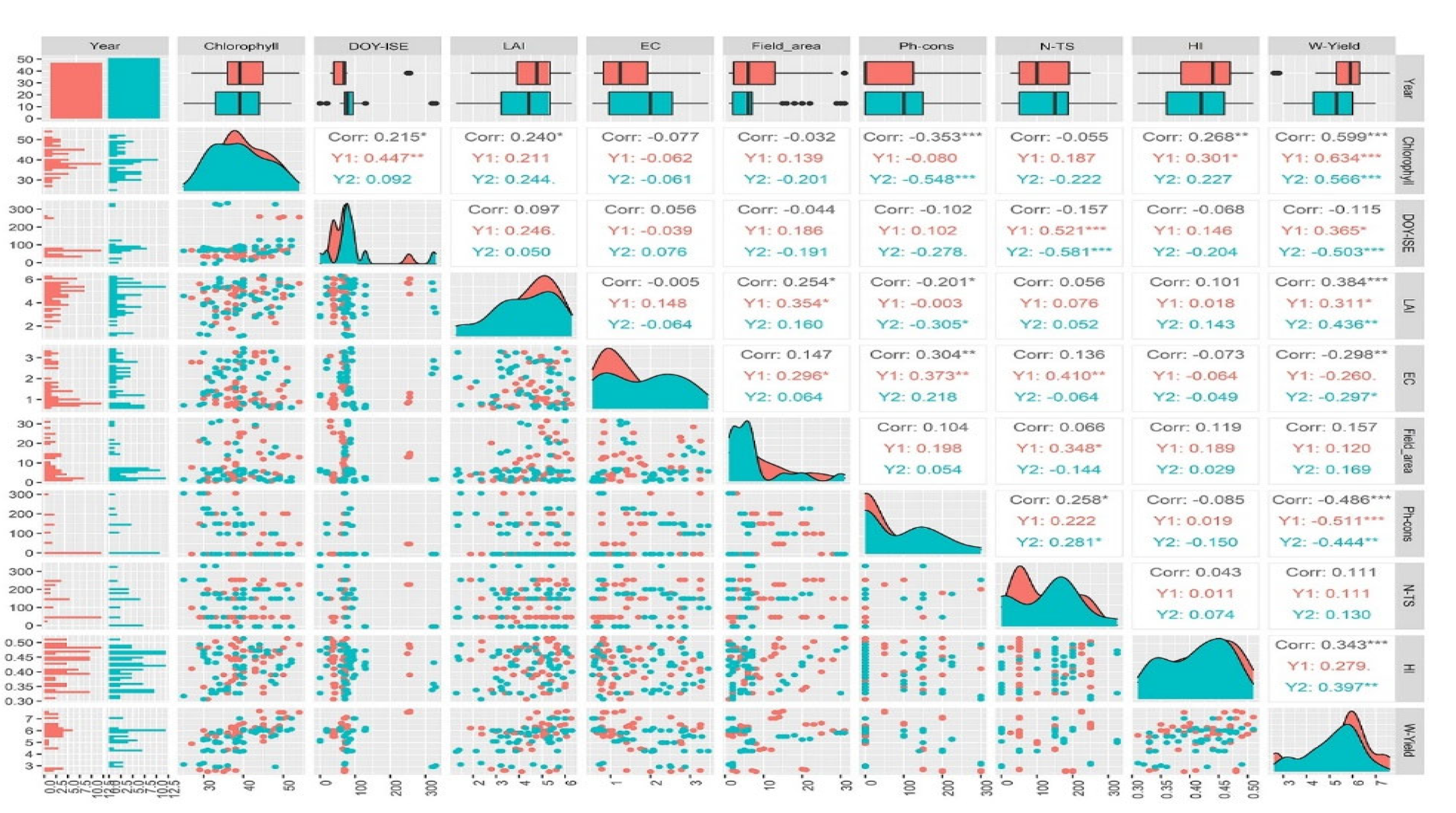
| Variables | Unit | Mean | Minimum | Maximum | SE | CV (%) |
|---|---|---|---|---|---|---|
| Farming experience | Year | 26.34 | 1 | 68 | 1.58 | 59.60 |
| Farmer age | Year | 45 | 18 | 83 | 1.45 | 32.04 |
| Seed rate | kg ha−1 | 253.57 | 175 | 375 | 4.17 | 16.29 |
| Sowing date | Day of year | 294 | 49 | 342 | 4.66 | 15.71 |
| Total Neutralizing Value | % | 18.12 | 11.24 | 43.89 | 0.60 | 33.16 |
| Soil phosphorus | ppm | 10.10 | 1.80 | 57.18 | 1.41 | 138.41 |
| Soil pH | pH | 8.18 | 6.03 | 8 | 0.08 | 10.63 |
| Organic carbon in soil | % | 0.61 | 0.14 | 1.23 | 0.03 | 54.09 |
| Nitrogen fertilizer | Number | 1.59 | 0 | 3 | 0.10 | 62.89 |
| Total nitrogen | kg ha−1 | 206.73 | 0 | 500 | 13.61 | 65.18 |
| Potassium | kg ha−1 | 10.45 | 0 | 100 | 3.01 | 285.16 |
| Number of irrigations | Number | 5.47 | 3 | 8 | 0.12 | 21.57 |
| Insecticide | Frequency | 0.85 | 0 | 2 | 0.06 | 67.05 |
| Insecticide volume | Liter ha−1 | 0.55 | 0 | 2 | 0.05 | 98.18 |
| Herbicide | Frequency | 0.85 | 0 | 2 | 0.07 | 84.70 |
| Herbicide volume | Liter ha−1 | 0.75 | 0 | 2 | 0.06 | 81.33 |
| Length of growing period | Day | 226 | 120 | 260 | 2.58 | 11.32 |
| Harvesting duration | Start of spring | 86.07 | 61 | 109 | 0.79 | 9.09 |
| Wheat yield | kg ha−1 | 5377 | 2600 | 7600 | 0.12 | 0.02 |
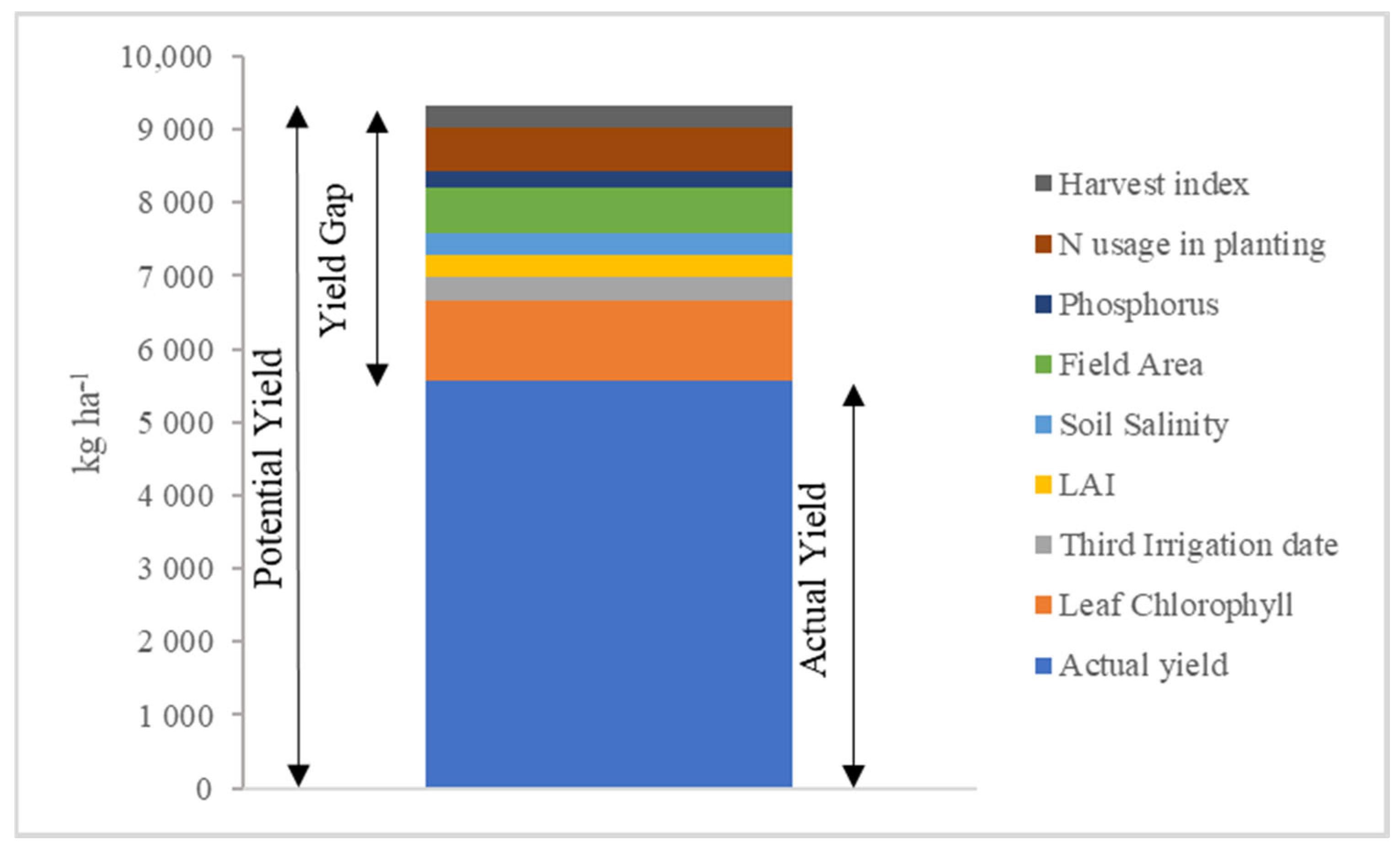
| Variables | Coefficients | CPA Model Variables | Predicted Yield | Yield Gap (Kg ha−1) | Yield Gap (%) | |||||
|---|---|---|---|---|---|---|---|---|---|---|
| Unit | Min | Mean | Max | Best | Mean | Best | ||||
| Leaf Chlorophyll Content (X1) | µgcm−2 | 75 | 25 | 39.47 | 54 | 54 | 2960 | 4050 | 1089 | 29 |
| Irrigation Stem Extension (X2) | DOY | −4 | 1 | 83.64 | 329 | 1 | −334 | −4 | 334 | 9 |
| LAI (X3) | 153 | 1.27 | 4.4 | 6.29 | 6.29 | 673 | 962 | 289 | 7.7 | |
| Soil Salinity (X4) | dSm−1 | −275 | 0.55 | 1.68 | 3.45 | 0.55 | −462 | −151 | 313 | 8.2 |
| Field Area (X5) | ha | 27 | 1 | 8.34 | 31 | 31 | 225 | 837 | 612 | 16.3 |
| Phosphorus (X6) | kg | −3 | 0 | 74.84 | 300 | 0 | −224 | 0 | 225 | 6 |
| Nitrogen at Tillering stage (X7) | kg | 3 | 0 | 126.88 | 325 | 325 | 380 | 975 | 594 | 16 |
| Harvest index (X8) | 3151 | 0.31 | 0.42 | 0.51 | 0.51 | 1323 | 1607 | 292 | 7.8 | |
| Wheat yield (kg ha−1) | kg ha−1 | – | 2600 | 5377 | 7600 | – | 5568 | 9316 | 3748 | 100 |
Disclaimer/Publisher’s Note: The statements, opinions and data contained in all publications are solely those of the individual author(s) and contributor(s) and not of MDPI and/or the editor(s). MDPI and/or the editor(s) disclaim responsibility for any injury to people or property resulting from any ideas, methods, instructions or products referred to in the content. |
© 2023 by the authors. Licensee MDPI, Basel, Switzerland. This article is an open access article distributed under the terms and conditions of the Creative Commons Attribution (CC BY) license (https://creativecommons.org/licenses/by/4.0/).
Share and Cite
Laleh, K.M.; Ghorbani Javid, M.; Alahdadi, I.; Soltani, E.; Soufizadeh, S.; González-Andújar, J.L. Wheat Yield Gap Assessment in Using the Comparative Performance Analysis (CPA). Agronomy 2023, 13, 705. https://doi.org/10.3390/agronomy13030705
Laleh KM, Ghorbani Javid M, Alahdadi I, Soltani E, Soufizadeh S, González-Andújar JL. Wheat Yield Gap Assessment in Using the Comparative Performance Analysis (CPA). Agronomy. 2023; 13(3):705. https://doi.org/10.3390/agronomy13030705
Chicago/Turabian StyleLaleh, Kambiz Mootab, Majid Ghorbani Javid, Iraj Alahdadi, Elias Soltani, Saeid Soufizadeh, and José Luis González-Andújar. 2023. "Wheat Yield Gap Assessment in Using the Comparative Performance Analysis (CPA)" Agronomy 13, no. 3: 705. https://doi.org/10.3390/agronomy13030705