Management Effect on the Weed Control Efficiency in Double Cropping Systems

Abstract

There are often negative side-effects associated with the traditional (silage) maize cropping system related to the unprotected soil surface. Reducing soil disturbance could enhance system sustainability. Yet, increased weed pressure and decreased nitrogen availability, particularly in organic agriculture, may limit the implementation of alternative management methods. Therefore, a field experiment was conducted at two distinct locations to evaluate the weed control efficiency of 18 organically managed silage maize cropping systems. Examined parameters were relative weed groundcover (GC_weed) and its correlation with maize dry matter yield (DMY), relative proportion of dominant weed species (DWS) and their groups by life form (DWS_group). Treatment factors comprised first crop (FC—winter pea, hairy vetch, and their mixtures with rye, control (sole silage maize cropping system—SCS)), management—incorporating FC use and tillage (double cropping system no-till (DCS NT), double cropping system reduced till (DCS RT), double cropped, mulched system (DCMS Roll) and SCS control), fertilization, mechanical weed control and row width (75 cm and 50 cm). The variation among environments was high, but similar patterns occurred across locations: Generally low GC_weed occurred (below 28%) and, therefore, typically no correlation to maize DMY was observed. The number of crops (system), system:management and occasionally management:FC (group) influenced GC_weed and DWS_(group). Row width had inconsistent and/or marginal effects. Results suggest differences related to the successful inclusion of DCS and DCMS into the rotation, and to the altered soil conditions, additional physical destruction by shallow tillage operations, especially in the early season, which possibly acts through soil thermal and chemical properties, as well as light conditions. DCS RT could successfully reduce GC_weed below 5%, whereas DCS NT and particularly DCMS (Mix) suffered from inadequate FC management. Improvements in DCMS may comprise the use of earlier maturing legumes, especially hairy vetch varieties, further reduction/omission of the cereal companion in the mixture and/or more destructive termination of the FC.

1. Introduction

Silage maize production in Germany is at a continuously high level [1,2]. However, concerns about system sustainability are rising due to negative side effects associated with traditional maize production.

In temperate European conditions, under old/traditional organic management, the row crop maize is usually sown in early May, mostly with 75 cm row width into an autumn-ploughed soil (CT), often after a winter fallow. The crop has a high nitrogen (N) and temperature demand, a slow juvenile development, and therefore, a low competitive ability in the early season. Consequently, from the harvest operations/incorporation of the residues of the previous crop—be it a cover crop or not—until canopy closing of the maize crop (late June–July), the system leaves most of the soil surface open [3], which in turn increases the soil erosion risk and offers an open niche to weeds [4,5,6,7,8]. Thus, a series of intensive mechanical weed control operations are usually conducted [5,7], which further accelerates the soil erosion risk and increases the soil compaction risk [7,9]. Climate change may enhance these problems due to more variable local climates and the increased chance of weather extremes [10,11,12,13,14]. These difficulties are even more pronounced in organic agriculture, where tillage and mechanical weed control—also tightly connected to nutrient management—are an essential part of the (silage) maize production. The demand to reduce the tillage-based management in at least some phases of the crop rotation also reached the organic farming community [5,7]. A possible reduction of tillage practices at very demanding phases of the rotation—e.g., with row crops such as (silage) maize—may thus result in ecological benefits for the farming system [9].

Intending to reduce soil disturbance—partially related to mechanical weed control—several alternative systems have emerged. Some reduce the wide row width to accelerate the canopy closing [4,15,16]. Others use a winter cover crop [5,17], which may increase soil protection and weed control, while potentially reducing nutrient losses over the winter months [6,7]. Afterwards, the cover crop may be harvested (classical double cropping systems (DCS)) or it may be mulched to support the following maize crop (double cropped, mulched system—DCMS). Such alternative systems most often utilize cereals, legumes and their mixtures to balance the possible benefits and setbacks—e.g., nutrient, especially N dynamics, or soil cover [1,18,19,20,21,22]. In DCS, the tillage type after the cover crop harvest may further influence nutrient and weed management [7,17,23,24,25,26,27]. In DCMS, the soil is protected at least until the early development phase of the second crop [28]. The residue quality and quantity will determine the potential success of DCMS systems—e.g., plant available water and nutrients, especially N dynamics, cover crop regrowth and the success of maize sowing and development, along with the length of the vegetative window [3,8,19,21,22,28,29,30,31,32,33,34,35,36,37]. Under German conditions, leafy, wild-type winter pea, hairy vetch [3,21,28] and rye—alone or as a cereal companion—showed promising results [1,28].

Most of the research under organic conditions—comparing some of these alternative systems—concluded that the main challenge in organic (silage) maize production remains the weed management, which may hinder soil conservation practices [5,7]. Furthermore, weather and environment strongly influence the system-related possibilities/effects of weed management and crop yield development [4,5,24,25]. The researchers in the mentioned sources highlighted the importance of understanding the systems and interactions within.

For efficient weed control, not just the amount of weeds, but also the community itself is decisive [26,38]. Some recent comprehensive surveys on weed communities in maize cropping systems across Germany revealed that weed species most commonly associated with maize cropping—summer annuals such as Solanum nigrum L., Amaranthus spp.—are rather scarce, whereas other, more generalist species dominate the weed flora on many maize fields [39,40,41,42]. This could be partially due to the chosen methodology of early weed survey in maize BBCH 12–18 [39,41,42], as pointed out by Mehrtens et al. [41]. De Mol et al. [39] examined factors which could potentially shape the weed communities. They revealed similar results as previous examinations in other studies that the chosen characteristics (factors) fail to explain most of the variation. Nevertheless, from the amount of variation explained, environment—especially location, location:climate and location:soil interactions—had the strongest effect, whereas management could explain only a comparatively small amount of variation—mostly by rotation and, to a smaller extent, by tillage. Year had only a marginal effect on weed composition [39]. Similar results on the influence of rotation and tillage were found for community-averaged weed traits [43,44,45].

The cited research included some alternative systems (DCS and DCMS) with a special focus on weed control, whereas others surveyed maize fields under a broad range of management conditions. Only a few articles reported factor effects on weed communities as a whole—e.g., [38,40,41]—rather than focusing on one or a couple of weed species—e.g., [31,32,46,47]—or purely on weed biomass, density, diversity indices or community-averaged weed traits to describe the community under different management conditions—e.g., [6,23,43,44,45].

An exact field experiment was conducted to assess management effects and their interactions on maize yield and weed development. Here, various combinations of tillage-reduced weed management were compared at two locations over two years. The study aimed to compare alternative management systems—different winter cover crops, management (DCS with RT or NT, DCMS) and row width—to a sole silage maize cropping system (SCS) [3].

The focus of this article lies on the relative weed control efficiency—groundcover (GC_weed), dominant weed species (DWS) and their groups by life form (DWS_group). The objectives of the analysis are to measure the main factor effects (FC, management and row width) and to help the understanding of guiding principles by evaluating interactions among treatment factors and with localities. The following major hypotheses were defined for the study: Under organic management and during the vegetative maize development phase, (1) GC_weed in DCS and DCMS is comparable to SCS; (2) GC_weed is strongly influenced by tillage with the expected pattern DCMS < DCS RT < DCS NT; (3) similarly, GC_weed is lower in DCMS with legume–cereal mixtures than in DCMS with pure legume stands; and (4) GC_weed is reduced with reduced row width, irrespective of other factors. Additionally, (5) GC_weed reduces maize dry matter yield and finally, (6) DWS_(groups) are altered by DCS and DCMS compared with SCS.

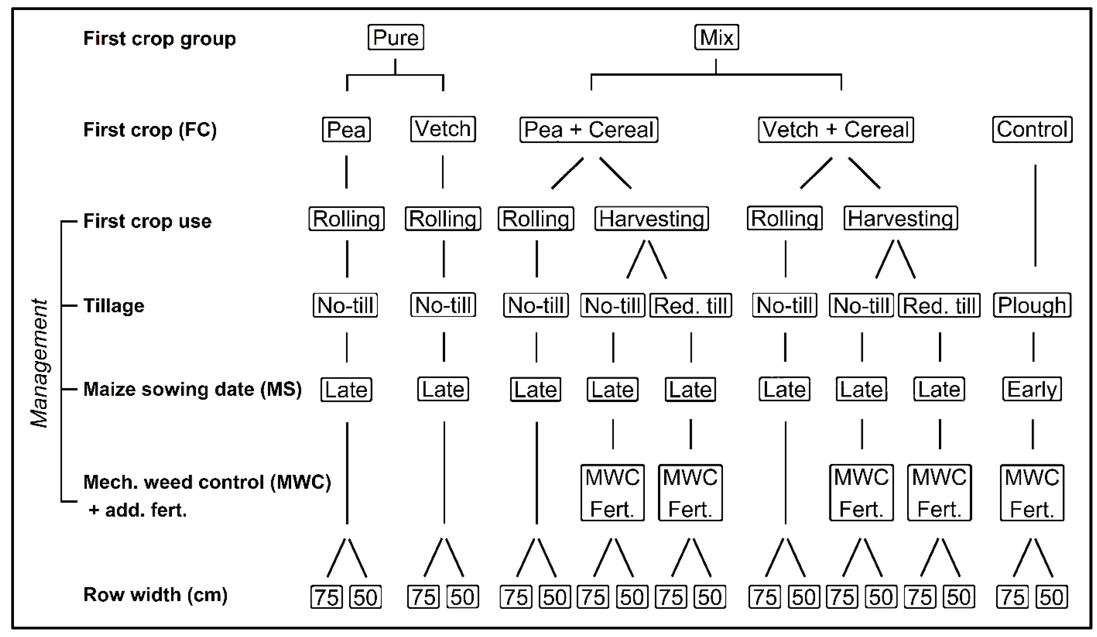
2. Materials and Methods

A field experiment was conducted at two German locations (Trenthorst, Schleswig-Holstein (TRE, N 53.76667 E 10.51667, 40 m above sea level (ASL)) and Neu-Eichenberg, Hessen (NEB, N 51.37936 E 9.91365, 247 m ASL)) in two consecutive years (2019–2020 and 2020–2021) to investigate the weed control efficiency of alternative silage maize cropping systems under organic management. The locations have similar soil type (luvisols), but they have different weather patterns with an average annual temperature and cumulative precipitation of 9.1 °C and 690 mm at TRE, as well as 9.3 °C and 638 mm at NEB. For more information, see Schmidt et al. [3].

The experiment followed a row-column design (4 × 20 units with net 30 m² plots) with four replications, and included 18 shared treatments tested at both locations, comprising alternative silage maize cropping systems, collected under the terms double cropping system (DCS) and roller-crimper terminated, double cropped, mulched system (DCMS), as well as the sole silage maize cropping system (SCS) as a control to represent common farming practices. Factors ranged from first crop (group) (FC (group)—pure winter pea (P) or hairy vetch (V) and their mixtures with a cereal partner (V-Mix, P-Mix), control), management—grouping factor comprising tillage (RT, NT, Roll and CT), additional slurry fertilization (yes-no), mechanical weed control (MWC; yes-no) and row width (75 cm and 50 cm) in a non-orthogonal and unbalanced manner. Please note that the maize sowing date was adjusted to optimize systems to the number of crops—in SCS, maize was sown earlier than in DCS and DCMS—hence any difference among SCS and DCS, DCMS is also based on the combined effect of the maize sowing date and the presence of winter cover crop. Factors and their combinations are described in Figure 1. For clarity, discussed factors are written in italics throughout the paper [3].

The weather conditions varied in the two experimental years: 2019–2020 was relatively dry, especially near the maize sowing and establishment phases. On the other hand, the weather was exceptionally cool and humid for the aforementioned phases in 2020–2021. For more detailed information, see Schmidt et al. [3].

All plots were prepared with conventional tillage (CT) in autumn (September–November). First crops (FCs) were sown briefly after and were harvested or rolled in early-to-full bloom between the end of May and the beginning of June. Maize was sown shortly after with non-inversion tillage (DCS RT) or no tillage (DCS NT, DCMS) practices. Maize in the control plots (SCS) was sown earlier (beginning of May) after a shallow soil preparation just as for DCS RT. In 2020–2021, there was a ca. 1 month delay of maize sowing in SCS at TRE due to weather circumstances. FC varieties were identical across locations, but maize varieties were adjusted for best results for each location. DCS and SCS were slurry-fertilized in the first four weeks of sowing (60–80 kg N ha⁻¹, location-specific) and hoed on average two times per season (see Schmidt et al. [3] Table A2 for specificities). In the DCS 50 cm treatments at NEB, no MWC could be conducted in 2020–2021. Maize harvesting took place in September–October at BBCH 83–87. In the first experimental year at TRE, a shallow soil disturbance before maize sowing was performed in every DCS plot, and therefore eliminated DCS NT from the experiment (and doubled the representation of DCS RT) [3]. See Schmidt et al. [3] (Appendix A) for more information on the locations, experimental conduct and experimental design.

Weed control efficiency was assessed through the ratio of weed groundcover to maize groundcover development (GC_weed) and dominant weed species development (DWS, presence-absence), also grouped by life form (DWS_group), related to the groundcover of each species over time. Generally, only one species was selected as DWS (presence), whereas the other species were recorded as absent (not the DWS) for each time-step. The measurements took place on three 0.5 m × 0.5 m permanent quadrats. Quadrats were fully randomized between two rows in the first year (2019–2020), whereas they were always edging a row in the second year (2020–2021). The measurements took place in a two-week rhythm from the silage maize sowing date in the DCS and DCMS systems until canopy closing in the respective plot, giving ca. four repeated measurements in SCS and ca. five in DCS and DCMS (see

Table A1. Measurement dates (t_i) in days after sowing (DAS, d) for each treatment. (TRE = Trenthorst, NEB = Neu-Eichenberg; SCS = sole cropped system, DCS = double cropping system, DCMS = double cropped, mulched system, 75 cm = 75 cm row width of maize, 50 cm = 50 cm row width of maize).

Location	Year	Distinct Factors	t0	t1	t2	t3	t4	t5	t6
TRE	2019–20	SCS	0	57	71	85
		DCS, DCMS	0	10	24	38	52	66	80
	2020–21	SCS	0	14	29	40	54	70	85
		DCS	0	8	23	34	48	64	79
		DCMS	0	9	20	34	50	65
NEB	2019–20	SCS	0	36.5	50
		SCS, row 1	0	13.5	28	41.5	55.5
		DCS, DCMS	0	13.5	28	41.5	55.5	75.5
	2020–21	SCS	0	48	63	76.5	90.5
		DCS 75 cm	0	23	38	51.5	65.5
		DCMS	0	15	30	43.5	57.5
		DCS 50 cm	0	10	25	38.5	52.5

for more information).

This methodology (DWS on a dependent multinomial scale) only assesses the most dominant species per treatment and does not relate 1:1 to the intact weed community. Species may have been consistently present in a treatment, yet never to the extent to be the DWS. Thus, the evaluation has three important limitations: (1) Results are dependent. If a species or group is highly represented, other species or groups will be less represented. Therefore, each group (or species) needs to be seen as a part of the whole community—here, the DWS community. (2) Introduced species (FC) and the natural vegetation were not distinguished from each other for DWS, due to their dependent nature and potential competition with maize. (3) Results only show the DWS community and not the intact/full community structure of the field, as the proportion of DWS and not the proportion of all observed weed species were measured. Nevertheless, this methodology allows a focused comparison of treatments, with only the most thriving species being considered.

Data were organized, graphically presented and statistically analyzed with Microsoft Excel 2016 and R version 4.0.4 [48] through RStudio version 1.4.1106 [49].

Due to subsampling and the time series nature of the data, pre-processing was carried out prior to statistical analysis. GC_weed was averaged over each plot and summarized over time according to the relative area under the disease progress stairs (AUDPS) process [50]. The relative proportion of DWS was calculated within a plot and summarized over time with the relative AUDPS process. DWS values were again adjusted to give a plot sum of 1. The resulting DWS dataset contained nearly 95% zero values in each location; therefore, species were grouped by life form—according to [51]—into four groups (DWS_group): (1) winter annuals (primary emergence in autumn), (2) summer annuals (primary emergence in spring), (3) winter-summer annuals (similar emergence in autumn and spring) and (4) biannuals-perennials for modelling and statistical analysis. Further information on measuring GC_weed and the data preparation can be found in Appendix B, whereas all species and their respective groups are listed in

Table A3. Average representation of the species (%) on the field averaged over year in each DWS_group at the locations. Sum of total species is put into parentheses and differentiated between more common and seldom (below 1% representation on the field) species.

Life form (DWSgroup)	Location (Total Species)	DWS (%)	Percent of Total (%)
winter annuals	TRE (4)	Vicia villosa Roth (10), Pisum sativum L. (6), × Triticosecale Wittm. ex A. Camus (4), Secale cereale L. (3)	23
	NEB (4)	Vi. villosa (16), Pi. sativum (9), Se. cereale (7), × Triticosecale (5)	37
summer annuals	TRE (5 + 2)	Lamium purpureum L. (19), Poa annuaa L. (2), Chenopodium polyspermum L. (1), Persicaria spp. b (1), Capsella bursa-pastoris c (L.) Medik. (1), Fallopia convolvulus (L.) Á. Löve (<1), Viola arvensis Murray (<1)	24
	NEB (3 + 4)	Fa. convolvulus (10), Chenopodium album L. (5), Persicaria lapathifolia (L.) Gray (4), Pe. maculosa Gray (<1),Ca. bursa-pastorisc (<1), La. purpureum (<1), Vi. arvensis (<1)	19
winter-summer annuals	TRE (6 + 2)	Veronica spp. d (10), Matricaria spp. e (10), Myosotis arvensis f (L.) Hill (8), Stellaria media (L.) Vill. (7), Alopecurus myosuroides Huds. (5), Galium aparine L. (1),Geranium rotundifolium L. (<1), Thlaspi arvense L. (<1)	41
	NEB (9 + 4)	My. Arvensisf (10), St. media (5), Aphanes arvensis L. (3), Ga. aparine (3), Matricaria chamomilla L. (2), Veronica persica Poir. (2), Ve. arvensis L. (1), Tripleurospermum inodorum (L.) Sch. Bip. (1), Th. arvense (1), Sonchus asper (L.) Hill (<1), Senecio vulgaris L. (<1), Lamium amplexicaule L. (<1), So. oleraceus L. (<1)	28
biannuals-perennials	TRE (4 + 4)	Lolium perenne L. (6), Equisetum arvense L. (1), Trifolium spp. g (1), Cirsium arvense (L.) Scop. (1), Rumex spp. (<1), Quercus spp. (<1), Cichorium intybus L. (<1), Taraxacum officinale F.H. Wigg. (<1)	9
	NEB (3 + 6)	Ci. arvense (8), Medicago sativa h L. (2),Rumex crispus L. (2), Solanum tuberosum L. (<1), Trifolium spp. (<1), Lolium multiflorum i Lam. (<1), Ru. obtusifolius L. (<1), Silene latifolia Poir. (<1), Ta. officinale (<1)	12

^a Poa annua is either summer annual or perennial (with a life span of only a few years). ^b Persicaria spp. are mainly Pe. maculosa and less abundantly Polygonum aviculare L. ^c Capsella bursa-pastoris is either summer annual or biannual. ^d Veronica spp. contains mainly Ve. persica and, less abundantly, Ve. agretis L. and Ve. arvensis. ^e Matricaria spp. contains mainly Tr. inodorum and, less abundantly, Ma. chamomilla, Ma. discoidea DC. and Anthemis arvensis L. ^f Myostois arvensis is either summer annual, biannual or winter annual. ^g Trifolium spp. at TRE mainly contained Tr. repens L. ^h Medicago sativa is either winter-summer annual or perennial. It is under the name Me. x varia Martyn (pro. sp.) in [51]. ⁱ Lolium multiflorum is winter annual, biannual or hapaxanth.

.

Based on Schaarschmidt and Vaas [52] and Piepho et al. [53], a generalized linear mixed effect model (GLMM) with a single fixed effect for all 18 treatment combinations (Figure 1) was fitted for both locations separately with a random effect for year (n = 2). This analysis provided mean estimates for GC_weed and each DWS_group across the two years. The model for GC_weed is:

treatment + year + (1|year:treatment) + (1|year:row) + (1|year:column)

(1)

with the notation: fixed + (1|random). Models were fitted with a beta distribution and cloglog (TRE) or probit (NEB) link. The models of each DWS_group followed a simplified structure:

treatment + year + year:row + (1|year:treatment)

(2)

with the notation: fixed + (1|random). Models fitted a quasibinomial distribution with logit link and binomial variance, allowing up to 981 iterations. More model specifications are listed in Appendix B.

Following Schmidt et al. [3], contrasts were employed to test hypotheses with three foci: (I) DCS and DCMS versus SCS (pseudo-one-factorial), (II) management factor (mixtures only) with FC or row width interactions and (III) FC factor (DCMS only) with row width interaction. Using these contrasts, main factor effects (management, FC and row width) and factor interactions were assessed graphically. Means were adjusted for unequal sampling when needed (e.g., at TRE). Confidence intervals for means, contrasts and pairwise differences were adjusted to control the family-wise type I error rate at 5% using the multivariate t (mvt) distribution [54]. The graphs presented for focus (I) allow an in-depth exploration of multi-way factorial interactions. Three-way and higher interactions were not considered in detail because they were often inconsistent.

Additionally, to assess year and year:treatment interaction effects, a model with both year and treatment as fixed effects was created. The model is

treatment + year + year:treatment + (1|year:row) + (1|year:column)

(3)

in the case of GC_weed with the following notation: fixed + (1|random). The year-wise model was fitted with a gamma distribution and inverse link for TRE, whereas it used a beta distribution and logit link for NEB. The corresponding model for individual DWS_group is

treatment + year + year:treatment + (1|year:row)

(4)

with the notation: fixed + (1|random). The model contained a random effect only for NEB, whereas for TRE, this was eliminated due to singularity issues. Hypotheses were tested similarly as mentioned above, including an additional year interaction (difference of differences for factor year), as described in Schaarschmidt and Vaas [52]. Further assessment of year:treatment interactions was conducted by a graphical inspection.

DWS_group model estimates were divided by the sum of all groups for each treatment to force the treatment sum to unity. Then, each raw species proportion was averaged over the years (including absences) and adjusted to their respective DWS_group proportion. The resulting DWS proportions were used to identify the species responsible for up to 75% of the total infestation in the individual treatments, excluding likely rare and underrepresented species with possibly strong spatial dependencies. This resulting subset of the data—also with DWS_group information—was used to compare locations and treatments.

A possible relationship between GC_weed and maize DMY was assessed visually using the raw data points. The details for maize dry matter yield (DMY, t ha⁻¹) quantified from silage-mature biomass samples dried at 105 °C can be found in Schmidt et al. [3].

The most important statistical packages used were: agricolae [55], glmmTMB [56], MASS [57], DHARMa [58], emmeans [59] and RVAideMemoire [60]. Further packages are listed and detailed information on the analyses can be found in Appendix B.

3. Results

In the following sections, results are discussed over location and year, followed by the three foci of the contrasts: (I) alternative systems versus control, (II) management factor and (III) FC factor.

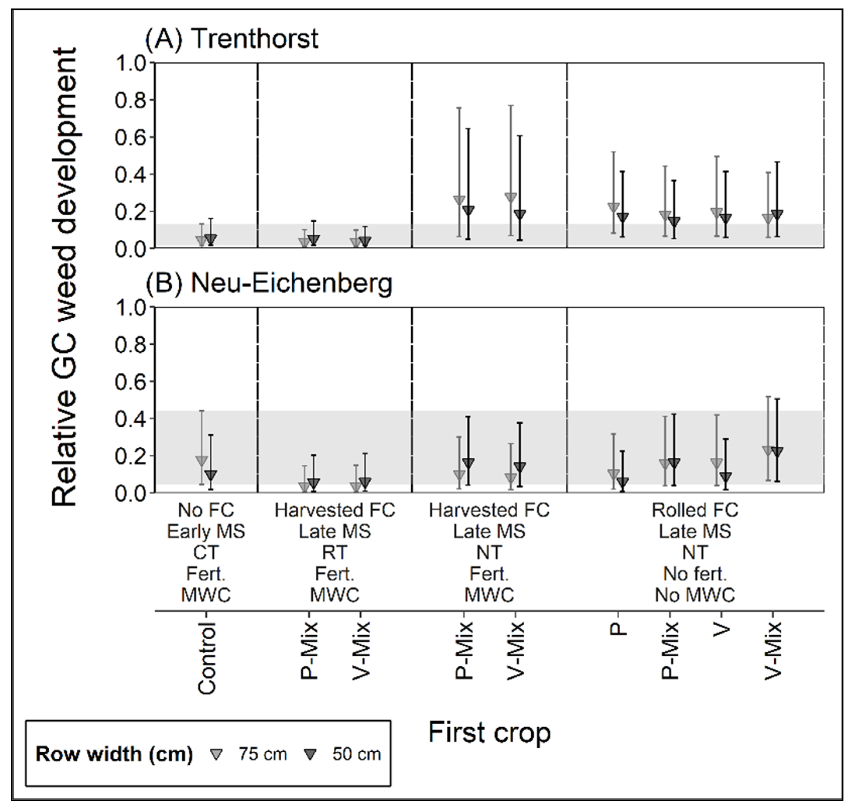
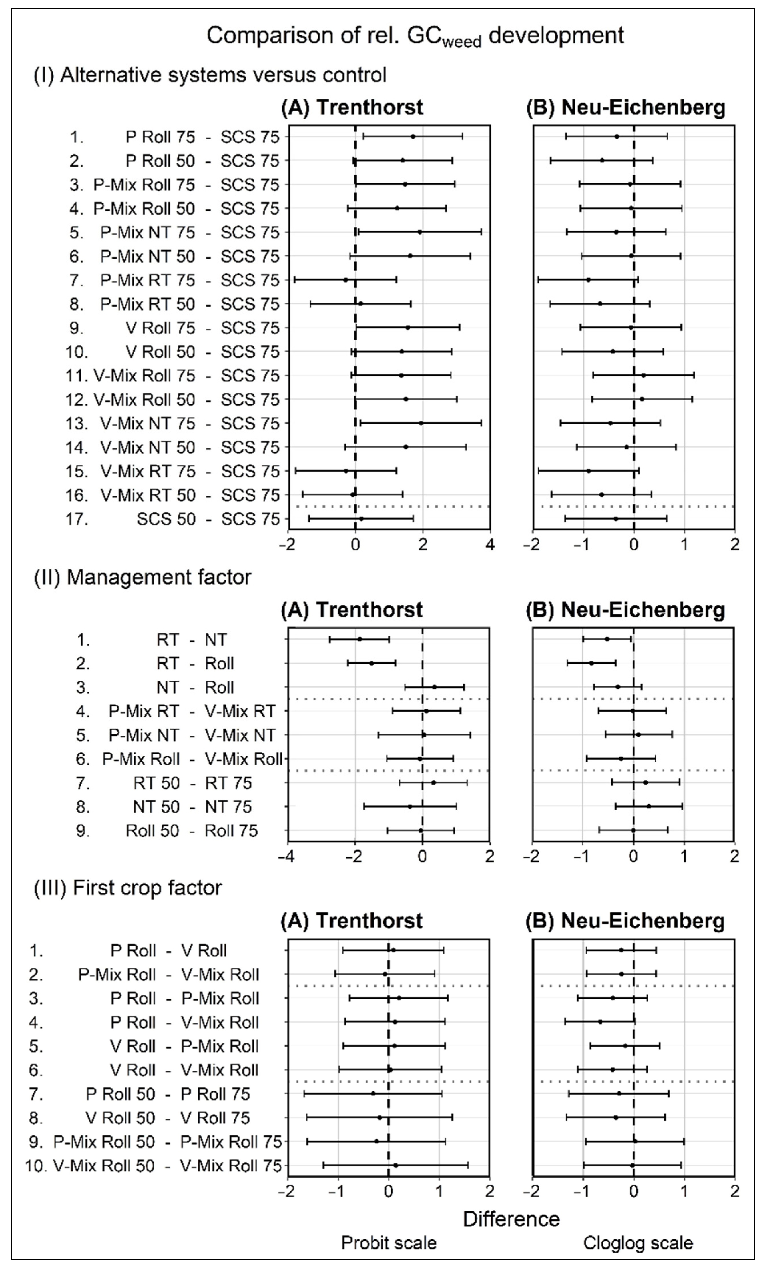
3.1. Relative Weed Groundcover Development

Relative weed groundcover development (GC_weed) was similar across locations and stayed below 0.28 (e.g., 28%) in all treatments (TRE: $\overline{\mathrm{x}}$ = 0.15, $\overline{\mathrm{sd}}$ = 0.08; NEB: $\overline{\mathrm{x}}$ = 0.12, $\overline{\mathrm{sd}}$= 0.06). The overall mean GC_weed difference in the second year compared with the first year was marginal (TRE: −0.05; NEB: 0.07).

Focus I: DCS/DCMS GC_weed compared with SCS were site-specific (significantly) higher (mostly part of TRE), statistically similar (partially TRE and mostly part of NEB) or non-significantly (NS) lower (partially NEB) (Figure 2 and Figure 3 part I). The reduced row width in SCS had no (TRE) or only a marginal effect (NEB). Despite the differences to the 75 cm SCS, factor effects behaved in a similar manner:

Focus II: Management was the most influential factor in the model at both locations, where RT significantly reduced GC_weed compared with NT and Roll (Figure 3 part II). NT was similar to Roll. There was no apparent two-way interaction between management and FC at any location and only a marginal interaction between management and row width at NEB (RT and NT suppressed slightly more weeds in maize with 75 cm row width).

Focus III: FC or FC group had little influence on GC_weed at both locations (Figure 3 part III). There was a slight trend at NEB with fewer weeds in Pure and in P(-Mix) versus V(-Mix). Row width had no (TRE) or marginal influence—only in DCMS Pure (NEB).

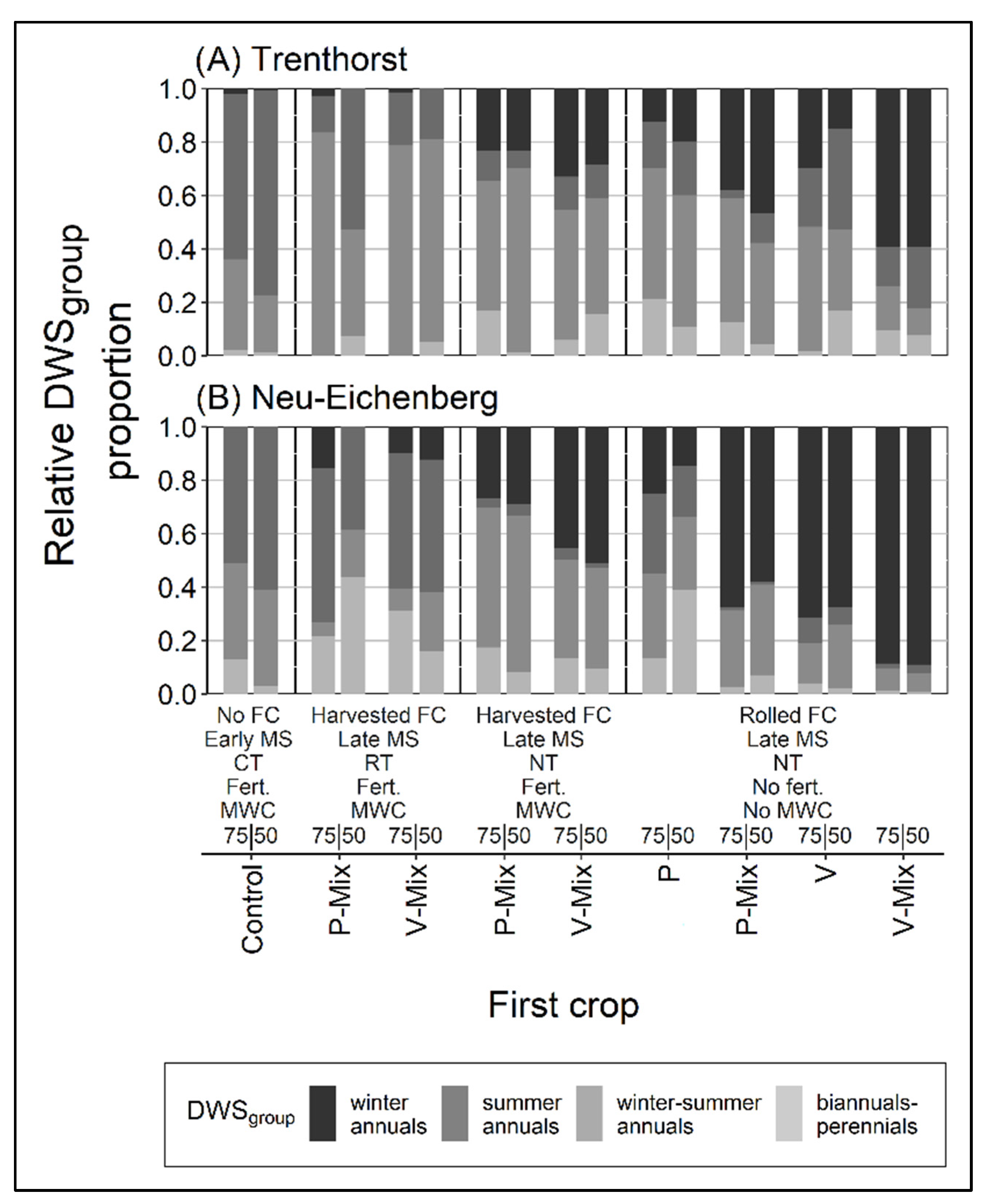
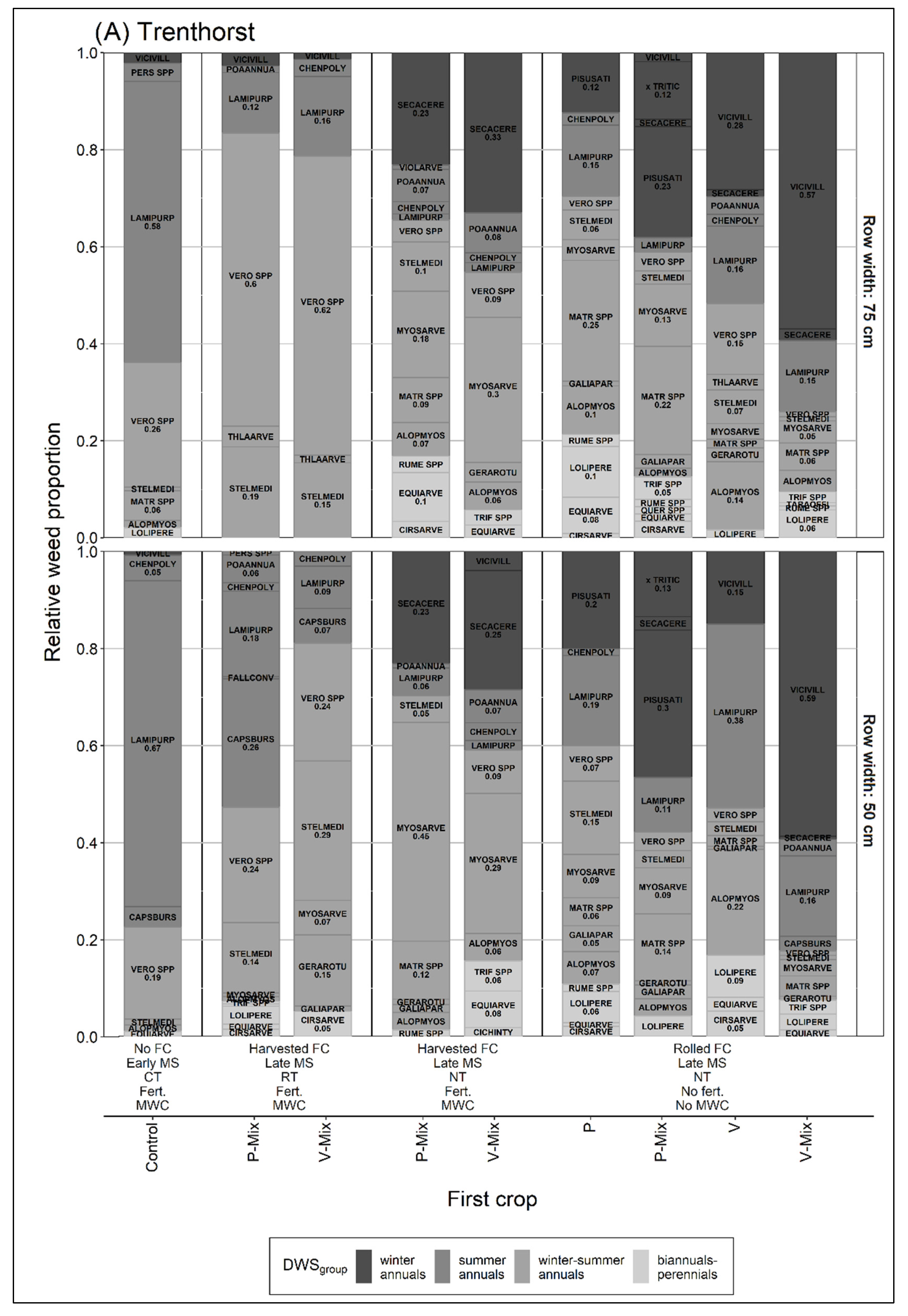
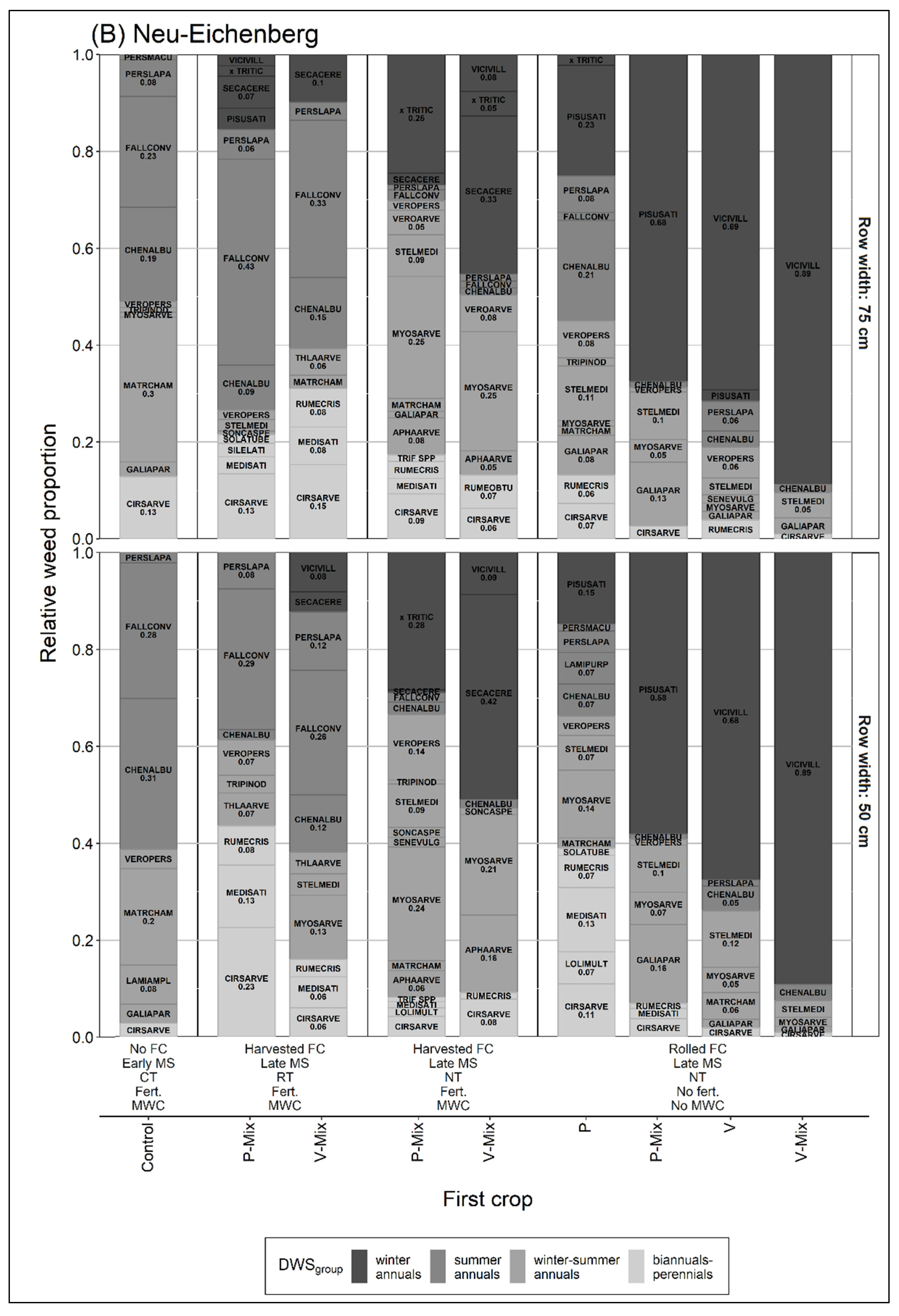
3.2. Relative Proportion of Dominant Weed Species Groups over the Season

In the following subsections, winter annuals—introduced species (FC)—are evaluated separately, as these species are part of DCS and DCMS. Summer and winter-summer annuals are discussed together, whereas biannuals-perennials are excluded from the comparisons due to low representation in the field, especially at TRE (

Table A2. Proportion of zero and one values of the raw datasets of each dominant weed species group (DWS_group) at each location and the iterations of the quasibinomial models. (TRE = Trenthorst, NEB = Neu-Eichenberg).

Location	DWSgroup	Proportion of Zero Values (%)	Proportion of One Values (%)	Model Iterations
TRE	winter annuals	50	0	980
	summer annuals	38	7	4
	winter-summer annuals	31	4	4
	biannuals-perennials	70	0	980
NEB	winter annuals	45	7	981
	summer annuals	46	5	3
	winter-summer annuals	42	3	981
	biannuals-perennials	58	1	895

). Figure 6 summarizes the results over every DWS_group. DWS and their respective groups are listed in Table A3, whereas their proportions are shown in Figure A3. After the first mention of the scientific names of individual species, the genus is abbreviated with two letters to exclude confusion among different genera. In species assemblages, the first species listed refers to the most abundant species. For example, in Veronica spp. (Ve. persica Poir., Ve. agrestis L., Ve. arvensis L.), it is Ve. persica. All other species are listed irrespective of their weight in the total abundance in the respective assemblage.

Measurements only assessed the most important genera per quadrat (one species). Therefore, results do not represent the intact weed community structure (see Section 2 for more detail).

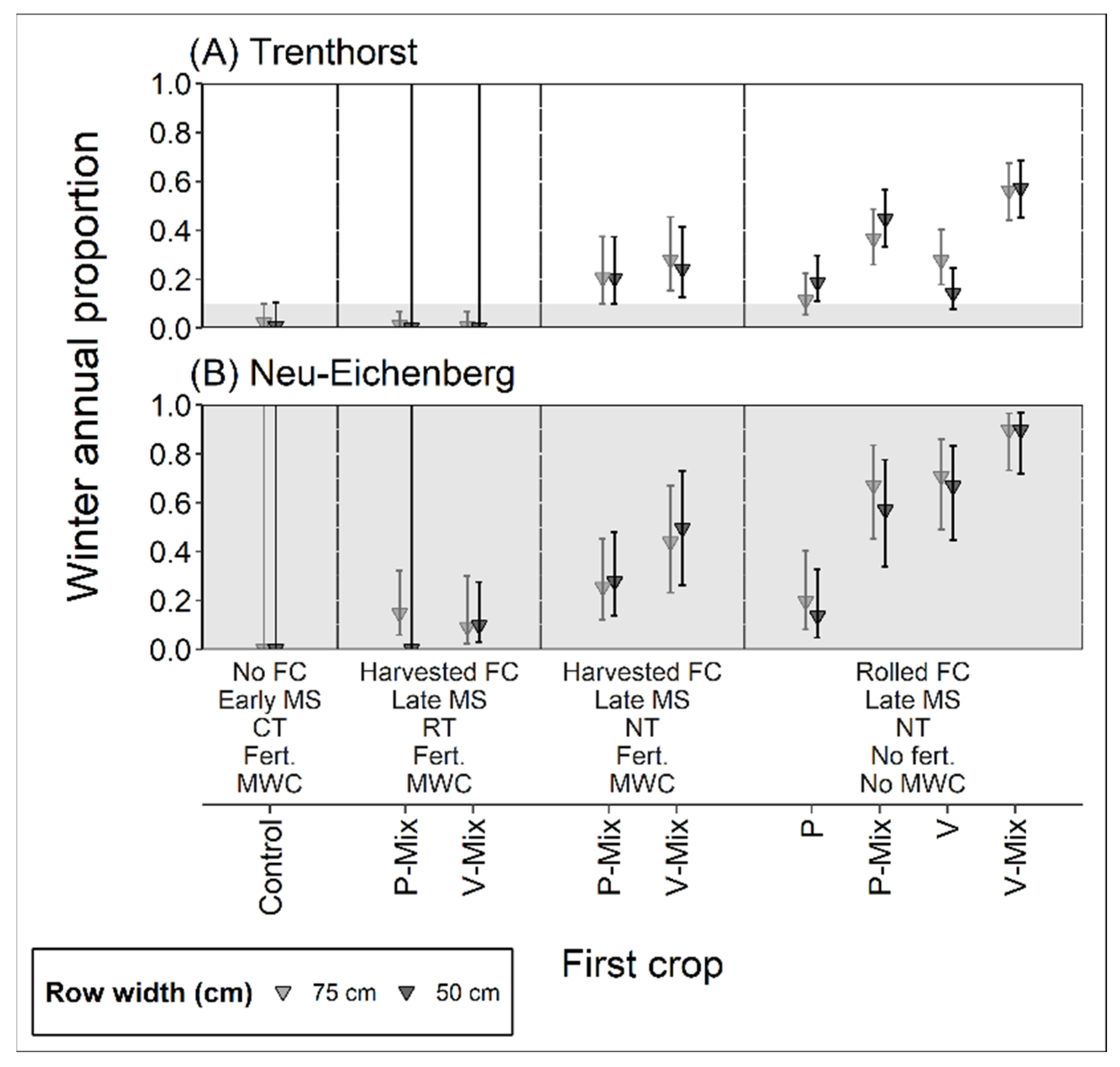
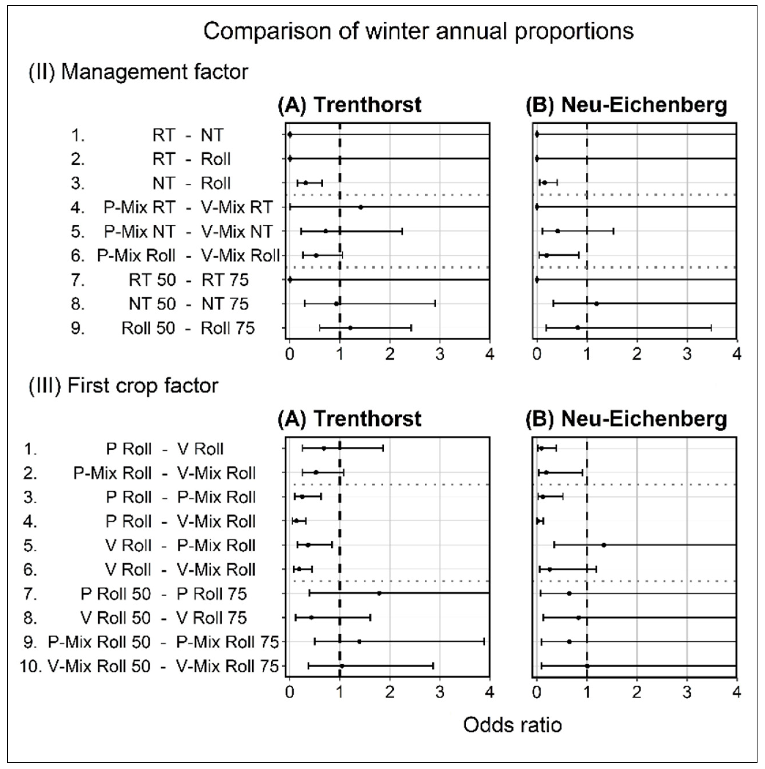
3.2.1. Relative Proportion of Winter Annuals

Winter annuals represented the FC (see Schmidt et al. [3] Table A3 for more information).

The relative proportion of winter annuals among the dominant weed species (DWS) ranged from 0.00 to 0.57 ($\overline{\mathrm{x}}$ = 0.20, $\overline{\mathrm{sd}}$ = 0.19) at TRE and from 0.00 to 0.90 ($\overline{\mathrm{x}}$ = 0.36, $\overline{\mathrm{sd}}$ = 0.31) at NEB. The overall mean proportion at NEB was 180% of that at TRE. A difference in overall mean winter annual proportion compared with the first year was absent at TRE (0.01) and positive at NEB (0.20).

Focus I: DCS/DCMS relative proportion of winter annuals compared with SCS was generally (significantly) higher, except for TRE DCS RT (Figure 4, see Appendix B for reasoning). The reduced row width in SCS naturally had no effect at either location. The factor effects behaved similarly across locations.

Focus II: Management was an influential factor in the model at both locations, in which RT strongly reduced the winter annual proportion compared with NT, which was also significantly more efficient in reducing winter annuals than Roll (Figure 5 part II). NT and RT rather promoted the cereals, whereas Roll favored the viny legumes (Figure A3). The two-way interaction of management with FC or row width was location-specific with similar patterns: For NT and Roll, P-Mix had fewer winter annuals (TRE and NEB). A similar pattern was observed in the RT treatments at NEB, whereas no apparent effect was detectable at TRE. There were only marginal interactions between management and row width.

Focus III: FC and FC group had substantial effects in DCMS at both locations (Figure 5 part III). Mixtures had higher winter annual species proportions than pure legumes. Furthermore, there was a trend of V(-Mix) being a more problematic FC, especially at NEB (significant differences). All DCMS had a considerable infestation of their respective legume species (Figure A3). Two-way interaction between FC and row width was mostly consistent (positive: TRE V, NEB P(-Mix), V; non-existent: V-Mix).

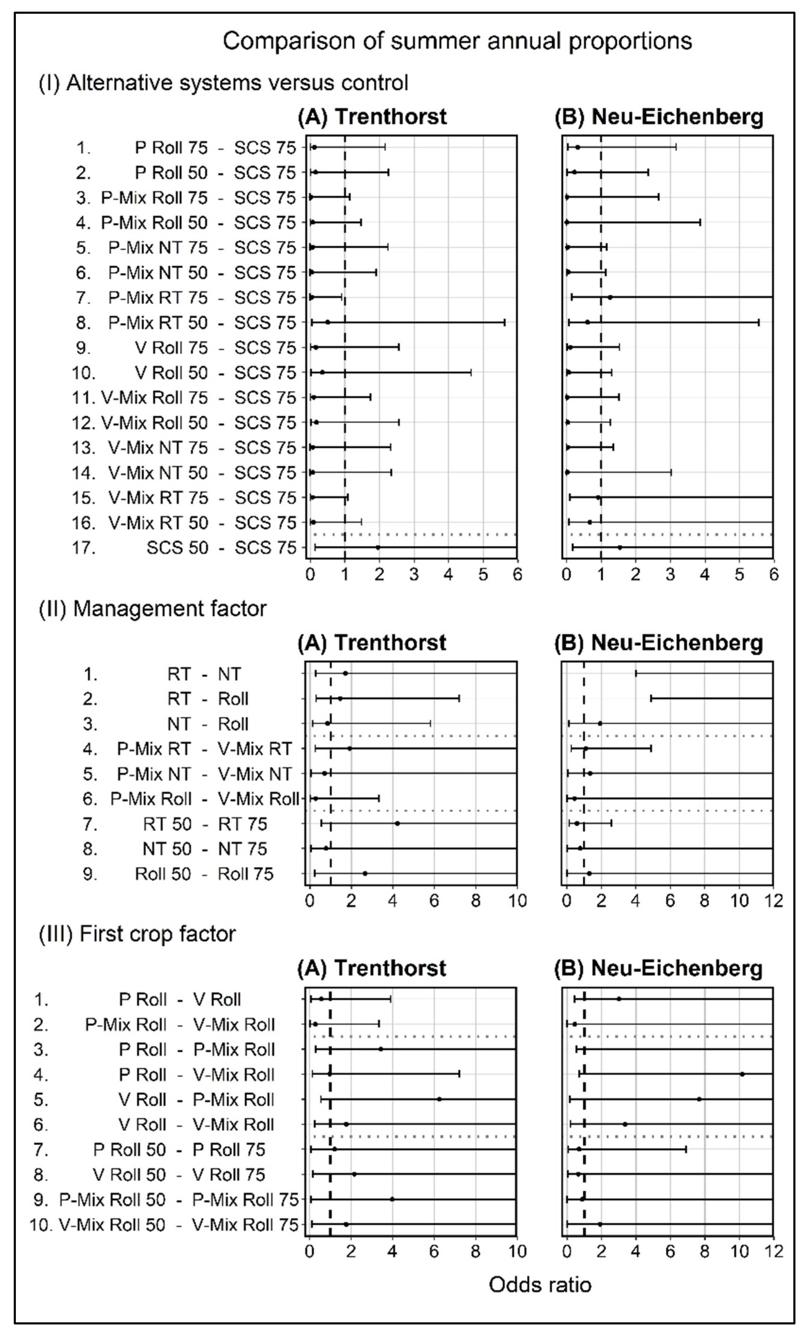
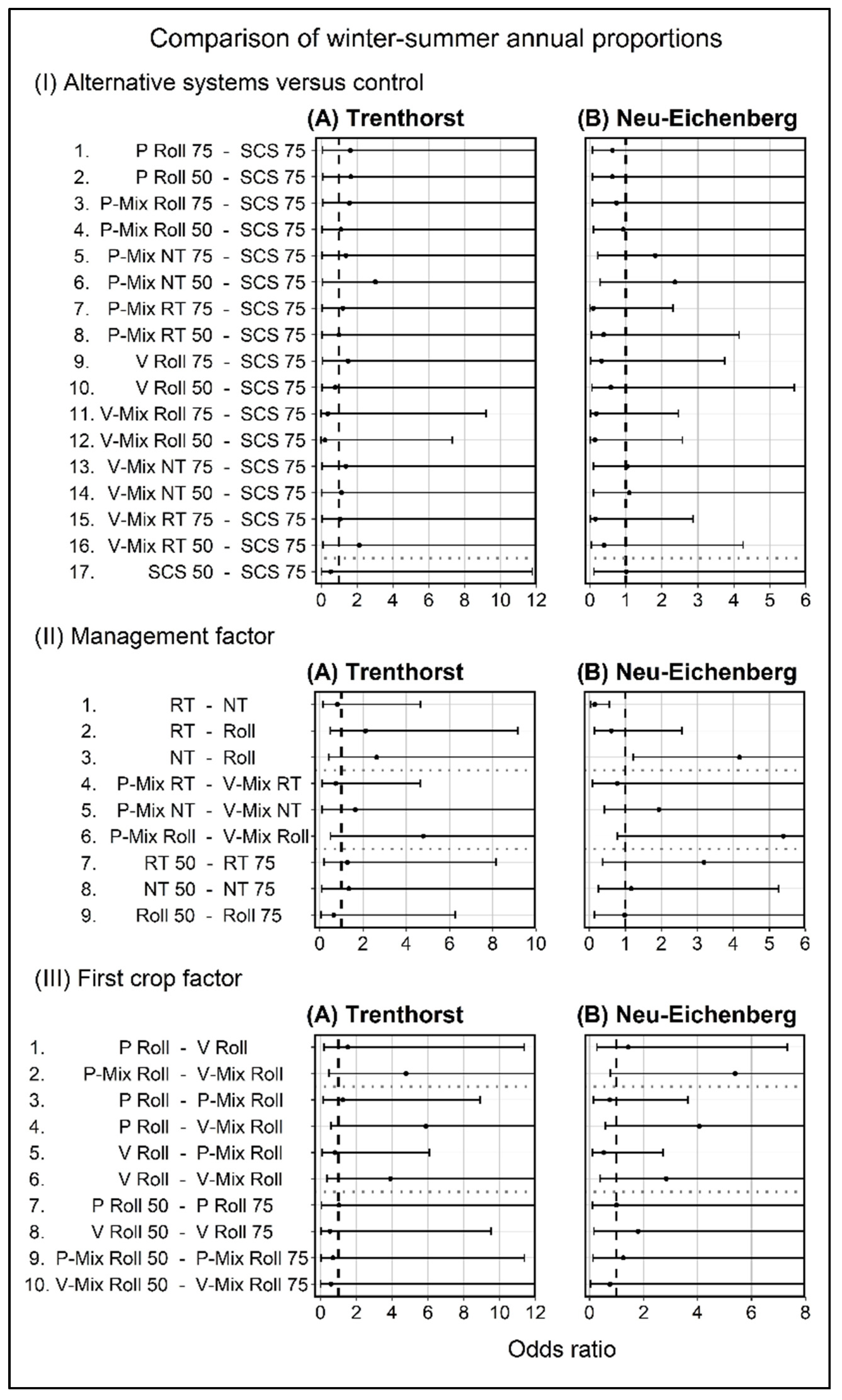
3.2.2. Relative Proportion of Summer and Winter-Summer Annuals

The two locations differed in DWS_group representation, but patterns were similar: More winter-summer annuals than summer annuals were present at both locations. There was an additionally large Lamium purpureum L. infestation (summer annual) at TRE, especially in the second year. The most important summer annual species were La. purpureum L., Poa annua L. and Capsella bursa-pastoris (L.) Medik. at TRE and Chenopodium album L., Fallopia convolvulus (L.) Á. Löve, Persicaria lapathifolia (L.) Gray and La. purpureum at NEB. The most important winter-summer annuals were Veronica spp. (Ve. persica Poir., Ve. agrestis L. and Ve. arvensis L.), Myosotis arvensis (L.) Hill., Matricaria spp. (Tripleurospermum inodorum (L.) Sch. Bip., Anthemis arvensis L., Matricaria chamomilla L. and Ma. discoidea DC.), Stellaria media (L.) Vill., Alopecurus myosuroides Huds. and Geranium rotundifolium L. at TRE, and My. arvensis, St. media, Ve. persica, Ma. chamomilla, Aphanes arvensis L., Galium aparine L. and Ve. arvensis at NEB.

The relative proportion of summer annuals among the DWS ranged from 0.03 to 0.75 ($\overline{\mathrm{x}}$ = 0.21, $\overline{\mathrm{sd}}$ = 0.20) at TRE and from 0.01 to 0.60 ($\overline{\mathrm{x}}$ = 0.20, $\overline{\mathrm{sd}}$ = 0.21) at NEB. The difference in overall mean summer annual proportion compared with the first year was positive at TRE (0.11) and absent at NEB (0.00). The relative proportion of winter-summer annuals among the DWS ranged from 0.10 to 0.61 ($\overline{\mathrm{x}}$ = 0.37, $\overline{\mathrm{sd}}$ = 0.12) at TRE and from 0.05 to 0.56 ($\overline{\mathrm{x}}$ = 0.26, $\overline{\mathrm{sd}}$ = 0.15) at NEB. The difference in overall mean winter-summer annual proportion compared with the first year was absent at TRE (0.07) and positive at NEB (0.26).

Focus I: Relative proportion of summer annuals in DCS/DCMS was lower compared with SCS, except for DCS RT at NEB (Figure A1 part I), whereas winter-summer annual proportions were slightly lower (NEB) or similar (TRE) to that of SCS (Figure A2 part I). Exceptions were DCS NT P-Mix (TRE only with 50 cm row width) with higher winter-summer annual proportions, DCS RT at NEB and DCMS V-Mix with lower proportions than SCS (TRE and NEB). Both locations had similar summer annuals in SCS and DCS RT—TRE: La. purpureum; NEB: Ch. album, Fa. convolvulus (Figure A3). Additionally, La. purpureum was present in DCMS at TRE. However, these species were not important in DCS NT at either location. Winter-summer annual species were only consistently similar to SCS in DCS RT at TRE (Veronica spp.). Row width in SCS had only marginal effects on both DWS_group and no detected effect on the species.

Focus II: Management was an influential factor for both summer annuals and winter-summer annuals at NEB, whereas at TRE, effects were more marginal with one distinct treatment (Figure A1 part II and Figure A2 part II). The resulting patterns were complementary over the two proportions—when one was higher, the other one would be lower—except in Roll V-Mix. Two-way interaction between management and FC was rather present for NT and Roll in winter-summer annuals for both locations, whereas no such interaction was detectable for summer annuals. Management:row width interaction had mostly marginal and inconsistent effects across locations. Summer annual species were present and shared between RT and Roll at TRE (La. purpureum), whereas at NEB, only RT showed a consistent presence of summer annuals (Fa. convolvulus, Ch. Album and Pe. lapathifolia), distinguishing itself from NT and Roll (Figure A3). Winter-summer annual species were different at both locations: at TRE, NT promoted My. arvensis, RT Veronica spp. and St. media, whereas Roll was associated with Matricaria spp. and My. arvensis (Figure A3). A slight pattern of DWS in management over different FC was present: Matricaria spp. and My. arvensis were more common in NT P-Mix and Roll P-Mix, whereas Veronica spp. were more frequently found in NT V-Mix and RT V-Mix. At NEB, NT also promoted My. arvensis, whereas RT promoted no winter-summer annual species. Roll had a strong interaction with FC: Roll V-Mix—just like in RT—did not promote winter-summer annuals, whereas Roll P-Mix promoted Ga. aparine and St. media. Additionally, St. media was the shared species for P-Mix over NT and Roll at NEB.

Focus III: The FC effect was relevant at both locations but to a different extent in different DWS_group (Figure A1 part III and Figure A2 part III). At TRE, summer annuals in pure legumes and in V(-Mix) had higher proportions than in mixtures or in P(-Mix). At NEB, pure legumes had a similar pattern of more summer annual infestation, but P had higher proportions than V or any mixture at this location. A consistent interaction between FC and row width was only present at TRE and over pure legumes at NEB. FC patterns in the winter annuals were also more consistent in magnitude: all treatments except V-Mix were similarly highly infested, whereas V-Mix had a low infestation. There were consistently no FC:row width interactions for P. However, a consistent reduction with 50 cm row width for all other treatments was found at TRE. Summer annuals species were similar at TRE (La. purpureum) but not at NEB, where a separation over FC group occurred: only pure legumes facilitated summer annuals, yet the species themselves were inconsistent (Figure A3)—except for Ch. album in P. From the winter-summer annuals, My. arvensis and Matricaria spp. were promoted by P-Mix, whereas Poaceae—Al. myosuroides, the summer annual Po. annua and the perennial Lolium perenne L.—were favored by pure legumes. At NEB, St. media seemed to be more promoted in P(-Mix), and additionally, Ga. aparine was more present in P-Mix than any other FC.

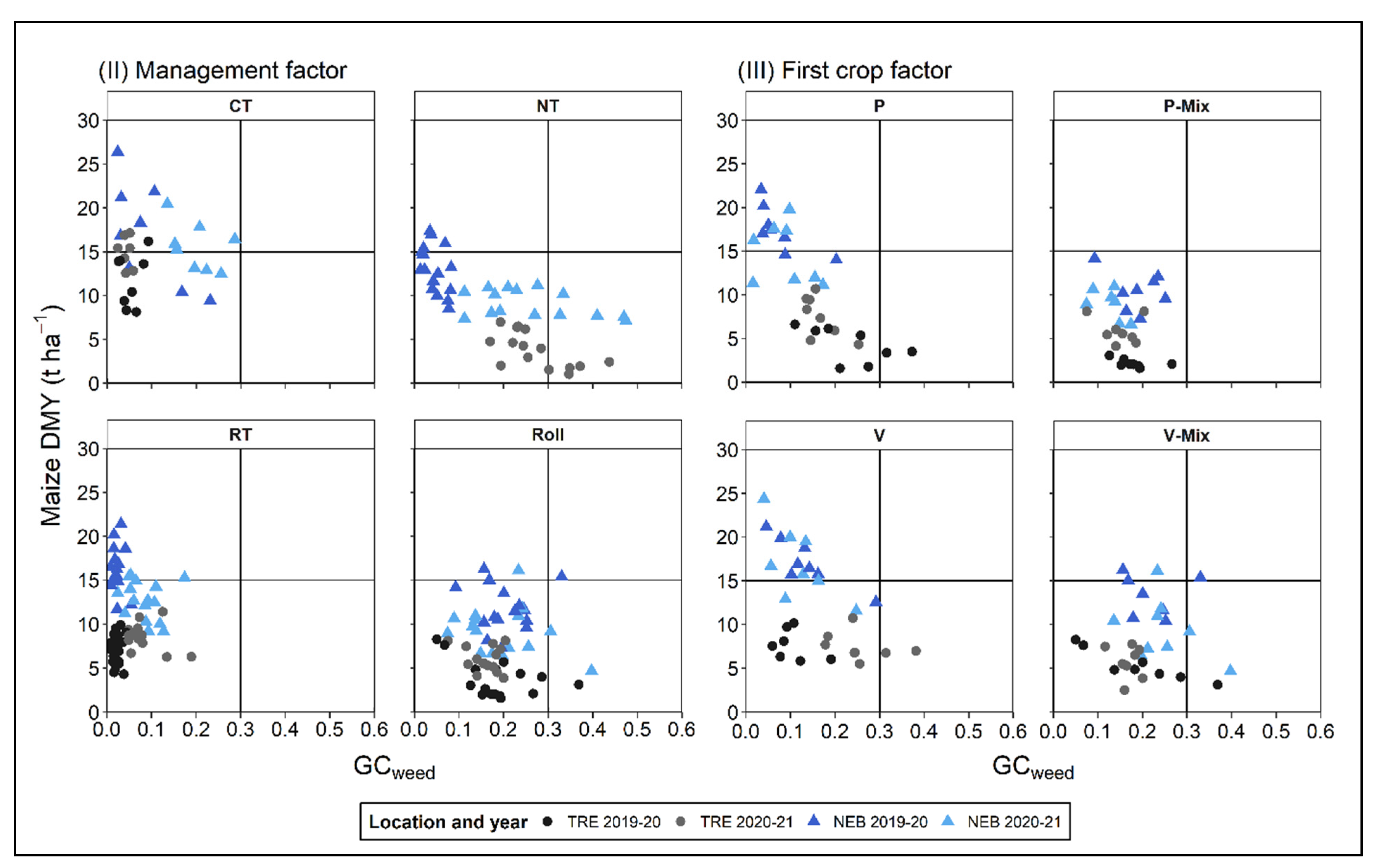
3.3. Relationship between Weed Groundcover and Maize Dry Matter Yield

Relative GC_weed over the season and maize dry matter yield had no detectable relationship with management, although an apparent negative relationship with some levels of FC—P, partially V and V-Mix—was present (Figure A4).

4. Discussion

Results varied across years and distinct locations for all measured parameters. Nonetheless, responses to management, partly to FC and row width were similar across locations, with an occasionally strong influence of year, as the two years under inspection differed throughout the maize cropping season. Consequently, year:treatment, year:location and year:location:treatment interactions regarding total weed presence and species composition were relevant for the measured parameters [39,40]. Differences may depend on the longer-term field history, relative quadrat location (relevant for 75 cm row width) and weather. Substantial weather differences were observed near maize sowing: 2020 was drier, whereas 2021 was cooler and rainier at both locations [3]. These differences influenced sowing dates and further possibilities of MWC (Schmidt et al. [3] Table A2), which likely affected weed presence and species composition. This resulted in no MWC at NEB for DCS in 50 cm row width in 2021. Furthermore, at TRE during 2020, no DCS NT treatment was present.

4.1. Relative Weed Groundcover Development

Weed groundcover (GC_weed) was low in all treatments over the two years and locations (estimates always below 0.28), with a relevant year effect only at NEB (highest estimate 52% higher in the second year compared with the first year). Treatments—maize and weed emergence, as well as development in general—were strongly influenced by spring soil conditions (e.g., water, temperature and mineralization-complex) [17,19,26,34,61,62,63,64,65]. See Schmidt et al. [3] for a more detailed explanation of these effects of the treatments at hand. These conditions relate to the system and management factors (SCS CT, DCS NT, DCS RT and DCS Roll). The patterns of GC_weed in these factor combinations were similar at both locations and years (DCS RT ≤ SCS CT ≤ DCS NT ≤ DCMS Roll) and were analogous to the effects observed in maize dry matter yield (DMY) of the same experiment [3], even if no apparent correlation of the two variables was present (Figure A4).

Both FC and row width had comparatively lower effects than system:management, but with mostly consistent directions over year and location: FC only influenced GC_weed at NEB, where FC regrowth was a serious problem (Figure 6), especially in mixtures and V. This coincided with the higher FC DMY at this location [3], which could have contributed to inadequate control of the FC with the roller-crimper. Furthermore, the early-to-full bloom stage of Vi. villosa may have been too early for a successful control of the species, corroborating the findings of Mischler et al. [33] but not by Parr et al. [22]. Thus, these treatments rather introduced weeds (FC) in the rotation. Consequently, the mulch effect on only the native weed infestation (GC_weed) cannot be evaluated in this experiment. Therefore, the differences between DCMS Pure and Mix regarding the physical boundaries posed on maize development [3] cannot be confirmed for weed development. The row width effect was consistent at each location over the two years, but they were—except for DCMS Pure—location-specific. Some artefacts near detection/model boundaries may be created (for TRE SCS CT, DCS RT and NEB DCS RT). Nevertheless, every SCS and DCS at NEB—in contrast to DCMS Pure—consistently showed higher weed infestations in reduced row width, while year influenced only the magnitude, due to the generally higher weed infestation in year 2020–2021, which was attributed to wet weather circumstances and resulted in suboptimal conditions for crop management. Results contradict previous findings [16,25], where a narrower row width reduced weed infestations. However, in this experiment, relative to row width, only two-thirds (75 cm) or the whole width (50 cm) between rows were sampled, which may have distorted results due to unequal representation of between-row space. Furthermore, the methodology differed between years, so results related to row width must be treated with caution. An additional, system-related error source was the missing MWC at NEB for DCS 50 in the wet and cool 2020–21. Two-way interactions of management:FC or management:row width were generally marginal.

4.2. Relative Proportion of Dominant Weed Species

As mentioned above, year:location may have influenced results due to the exact field location and field history, relative location of quadrats to row, as well as weather conditions. Additionally, the chosen methodology only allows a constrained comparison of treatments. The three crucial constraints are: (1) Each DWS and DWS_group is part of the whole. Therefore, individual results are dependent on the respective community composition; (2) the natural weed community and FC regrowth were evaluated on the same scale (DWS). Due to this, detecting a particular effect on the natural weed flora was limited in some cases. (3) Only the DWS community was evaluated and not the community of all observed weed species present in the fields. Therefore, caution is required when interpreting individual DWS responses to factor/factor level.

4.2.1. Relative Proportion of Winter Annuals

Relative proportion of winter annuals was greatly influenced by system (DCS and DCMS versus SCS) and further by both management and FC. Marginal regrowth was observed in RT, whereas NT and especially Roll had substantial FC regrowth. In NT, the problematic FC-component was the cereal partner, which could not be adequately destroyed without a shallow soil tillage. After the first MWC, proportions of FC in the weed flora were substantially reduced. In Roll, the legume partners could survive the rolling with roller-crimper in the mixtures—especially at NEB—possibly related to biomass production, machinery and FC phenology [33] (see Section 4.1). Termination problems prevailed at NEB even after using a Cambridge roller combined with the roller-crimper in 2020–2021. Therefore, a less aggressive, probably earlier maturing hairy vetch (and winter pea) variety, a further reduction or omission of the cereal companion in the mixtures and/or an improved destructive power by the roller-crimper (weight) may increase FC destruction success in DCMS.

4.2.2. Relative Proportion of Summer and Winter-Summer Annuals

Relative proportions of summer and winter-summer annuals were location-specific and highly influenced by year (data not shown). Rotations at both locations focused on summer and winter cereals (not maize) and moderately on legumes and grass-clover mixtures. Other crops, such as rapeseed or potato were occasionally present in the past 10 years. Therefore, one would expect a greater proportion of winter-summer annuals than summer annuals in the weed community [39,40,44].

At TRE in 2020–2021, the increase in summer annuals in the second year was probably related to the massive infestation of La. purpureum and from Po. annua, whereas the slight increase in winter-summer annuals could not be attributed to individual species. Summer annuals were also highly influenced by year at NEB—increased in DCS RT and SCS CT; decreased in DCS NT and DCMS—despite having no difference between grand means. Winter-summer annuals showed a complementary pattern, except in DCS RT and DCMS V-Mix, which both remained less infected by winter-summer annuals.

In the case of summer annuals, system (TRE) or system:management (NEB) explained most of the variation. The system-effect probably goes beyond the maize sowing date, as no differences were observed among early and late sown SCS at TRE (data not shown). Both SCS CT and DCS RT were made up of similar summer annuals, whereas DCS NT and DCMS had only a marginal summer annual presence, which suggests that the similarities in these groups may guide the DWS community for summer annuals. A logical explanation would be that summer annuals—such as Fa. convolvulus, Ch. album, Persicaria spp. and Ca. bursa-pastoris—have relatively high temperature requirements for emergence, which could be reached through shallow soil disturbance (seedbed preparation or MWC) [17,61,62,63], and their predominant emergence time coincides with related management steps in maize production [8,25,26,31,38,40]. This is supported by the fact that these species are rather well represented throughout the maize fields in Germany [41]. On the other hand, La. purpureum, as the most problematic species at TRE, could only be successfully reduced by DCS NT, suggesting that other mechanisms are also involved in the germination of La. purpureum which are not connected to soil disturbance or light conditions due to the difference among DCS NT and DCMS (Mix and Pure) [65]. Nevertheless, the FC group also had a location-specific strong effect on summer annuals: pure legume mulches facilitated (slightly) more summer annuals than the mixtures. At NEB, the strong overrepresentation of the Vi. villosa probably reduced the magnitude of this effect. This could be related to more differences, e.g., light, temperature and nutrient requirements for emergence and establishment that are hindered to a different extent in DCMS Pure and Mix [18,21,22,28,30,34].

Winter-summer annuals were more location-specific than any other DWS_group. At TRE, only DCMS V-Mix was different from all other treatments. Nevertheless, a slight variation was still present—following the pattern seen at NEB—which pattern could appear more pronounced with increasing yearly repetitions. At NEB, management affected the winter-summer annuals strongly, where especially DCS RT had consistently low infestations. Species followed a similar trend, with system:management-specific DWS communities in the group. Only one species assemblage—Veronica spp.—at TRE was shared by SCS CT and DCS RT. The apparently missing effect of SCS sowing date stays uncertain due to the steeply increased representation of Veronica spp. in year 2020–21, where SCS sowing dates were only one week apart. Nevertheless, similarly as for summer annuals, the common soil disturbance in the early season possibly promoted the emergence [17,61,62,63]. However, de Mol et al. [39] found that these species—mainly representing Ve. persica, such as in this experiment—prefer unploughed fields with high crop densities. Additionally, with the late maize sowing date, St. media presence—one of the most common species in maize fields [39,42]—increased in DCS CT, making it similar to DCS RT (data not shown). This species was also more represented in 2020–21. My. arvensis was the only species consistently represented at both locations in DCS NT. This species (phenotype) may require light for emergence, as suggested by their lower presence in disturbed or mulched plots. Nevertheless, both locations showed an interaction of management and FC for this species, suggesting a residue quality-based difference of the legumes. At NEB, winter-summer annuals were not promoted in DCS RT, possibly due to the higher proportion of summer annuals and biannuals-perennials. Despite the low GC_weed in DCS RT—therefore a generally good weed control—perennial weed species are still present in the DWS flora (Figure 6) and may cause problems throughout the rotation [25,44,66]. Next to management, FC also had a very strong effect, where V-Mix promoted fewer winter-summer annuals than any other FC. This is possibly related to the high presence of Vi. villosa (TRE and NEB) and La. purpureum (TRE). Furthermore, DCMS Pure promoted more Poaceae at TRE, irrespective of their DWS_group, possibly related to the efficient nutrient scavenging of these species [19,20]. Further patterns of management:FC, FC or FC group were also present (Matricaria spp., My. arvensis), suggesting similar possibilities as for My. arvensis discussed for management:FC.

4.3. Relationship between Weed Groundcover and Maize Dry Matter Yield

GC_weed and maize DMY had no apparent relationship with the management factor and only a partial relationship with FC (Figure A4). General weed infestation was indeed low relative to maize groundcover, which could result in low interspecies competition [25,67]. The high regrowth of legumes in the DCMS Mix also did not influence maize DMY consistently. However, due to the weather variation and low year:location combinations, no clear pattern only shows that in distinct conditions, this method did not find any clear evidence of a relationship between these variables [26]. Even if weed infestation did not influence maize DMY, there could still be a negative effect on the following crops if species can reproduce [25].

5. Conclusions

In this study, a wide scope of factor combinations were examined (FC, management and row width) on weed groundcover development (GC_weed) and short-term dominant weed species group (DWS_group—winter annuals, summer annuals, winter-summer annuals, biannuals-perennials) shifts, proportional to the community of DWS_group. Effects on some DWS could also be evaluated with care on representation in the field and year.

A high variation among environments (years and locations) occurred, yet patterns were similar across locations: Number of crops (system) and their interaction with management had the biggest influence on the measured parameters, followed by management and FC. Row width had location-specific and/or marginal effects. Weed infestation (GC_weed) was generally low, thus seemingly not influencing maize dry matter yield, despite the complementarity observed. A clear pattern in management, and/or system:management interaction was present for GC_weed and DWS_groups—for winter annuals (FC regrowth) and the natural weed flora (summer and winter-summer annuals). Differences were seemingly promoted by system-induced technical problems (FC regrowth) and the early soil disturbance (SCS CT and DCS RT versus DCS NT and DCMS), acting possibly through light, soil temperature and mineralization conditions. Individual DWS could be altered through management and management:FC interactions.

DCS RT was consistently offering good weed control while reducing the soil erosion risk to an extent. On the other hand, DCS NT and DCMS introduced weeds into the system (FC regrowth), due to the technical problems of FC destruction. Particularly DCMS should be further improved through earlier maturing FC varieties, reduction or omission of cereal companion in the mixture and/or more destructive termination to reduce system-induced weed problems. Further research in a similar context, assessing the intact weed community shifts throughout a rotation—before and after the alternative systems—is required to further evaluate the viability of these systems.

References

1. Graß, R.; Heuser, F.; Stülpnagel, R.; Piepho, H.P.; Wachendorf, M. Energy crop production in double-cropping systems: Results from an experiment at seven sites. Eur. J. Agron. 2013, 51, 120–129. [Google Scholar] [CrossRef]
2. FNR. Bioenergy in Germany: Facts and Figures 2020; Fachagentur Nachwachsende Rohstoffe e.V. (FNR): Gülzow-Prüzen, Germany, 2019. [Google Scholar]
3. Schmidt, F.; Böhm, H.; Piepho, H.; Urbatzka, P.; Wachendorf, M.; Graß, R. Management Effects on the Performance of Double Cropping Systems—Results from a Multi-Site Experiment. Agronomy 2022, 12, 2104. [Google Scholar] [CrossRef]
4. Reckleben, Y. Cultivation of maize—Which sowing row distance is needed? Landtechnik 2011, 66, 370–372. [Google Scholar]
5. Carr, P.M.; Mäder, P.; Creamer, N.G.; Beeby, J.S. Editorial: Overview and comparison of conservation tillage practices and organic farming in Europe and North America. Renew. Agric. Food Syst. 2012, 27, 2–6. [Google Scholar] [CrossRef]
6. Graß, R.; Scheffer, K. Direkt- und Spätsaat von Silomais nach Wintererbsenvorfrucht—Erfahrungen aus Forschung und Praxis. In Proceedings of the 7. Wissenschaftstagung zum Ökologischen Landbau, Wien, Austria, 23–26 February 2003; pp. 45–48. [Google Scholar]
7. Peigné, J.; Lefèvre, V.; Vian, J.F.; Fleury, P. Conservation agriculture in organic farming: Experiences, challenges and opportunities in Europe. In Conservation Agriculture; Farooq, M., Siddique, K.H.M., Eds.; Springer: New York, NY, USA; London, UK, 2015; pp. 559–578. [Google Scholar]
8. Herrmann, A. Biogas Production from Maize: Current State, Challenges and Prospects. 2. Agronomic and Environmental Aspects. Bioenergy Res. 2013, 6, 372–387. [Google Scholar] [CrossRef]
9. Reicosky, D.C.; Sauer, T.J.; Hatfield, J.L. Challenging Balance between Productivity and Environmental Quality: Tillage Impacts. In Soil Management: Building a Stable Base for Agriculture; Hatfield, J.L., Sauer, T.J., Eds.; American Society of Agronomy Soil Science Society of America: Madison, WI, USA, 2011; pp. 13–37. ISBN 9780891181958. [Google Scholar]
10. Finckh, M.R. Integration of breeding and technology into diversification strategies for disease control in modern agriculture. Eur. J. Plant Pathol. 2008, 121, 399–409. [Google Scholar] [CrossRef]
11. MEA Food. Ecosystems and Human Well-Being: Current State and Trends; Balisacan, A.M., Gardiner, P., Eds.; Island Press: Washington, DC, USA, 2005. [Google Scholar]
12. Döring, T.F.; Vieweger, A.; Pautasso, M.; Vaarst, M.; Finckh, M.R.; Wolfe, M.S. Resilience as a universal criterion of health. J. Sci. Food Agric. 2015, 95, 455–465. [Google Scholar] [CrossRef]
13. Wolfe, M.S.; Baresel, J.P.; Desclaux, D.; Goldringer, I.; Kovács, G.; Löschenberger, F.; Miedaner, T.; Østergård, H.; Lammerts van Bueren, E.T. Developments in breeding cereals for organic agriculture. Euphytica 2008, 163, 323–346. [Google Scholar] [CrossRef]
14. IPCC. Climate Change 2014: Synthesis Report; IPCC: Geneva, Switzerland, 2014. [Google Scholar]
15. Marín, C.; Weiner, J. Effects of density and sowing pattern on weed suppression and grain yield in three varieties of maize under high weed pressure. Weed Res. 2014, 54, 467–474. [Google Scholar] [CrossRef]
16. Mhlanga, B.; Chauhan, B.S.; Thierfelder, C. Weed management in maize using crop competition: A review. Crop Prot. 2016, 88, 28–36. [Google Scholar] [CrossRef]
17. Peigné, J.; Ball, B.C.; Roger-Estrade, J.; David, C. Is conservation tillage suitable for organic farming? A review. Soil Use Manag. 2007, 23, 129–144. [Google Scholar] [CrossRef]
18. Snapp, S.S.; Swinton, S.M.; Labarta, R.; Mutch, D.; Black, J.R.; Leep, R.; Nyiraneza, J.; O’Neil, K. Evaluating cover crops for benefits, costs and performance within cropping system niches. Agron. J. 2005, 97, 322–332. [Google Scholar] [CrossRef]
19. Dabney, S.M.; Delgado, J.A.; Reeves, D.W. Using winter cover crops to improve soil and water quality. Commun. Soil Sci. Plant Anal. 2001, 32, 1221–1250. [Google Scholar] [CrossRef]
20. Fageria, N.K.; Baligar, V.C.; Bailey, B.A. Role of cover crops in improving soil and row crop productivity. Commun. Soil Sci. Plant Anal. 2005, 36, 2733–2757. [Google Scholar] [CrossRef]
21. Holderbaum, J.F.; Decker, A.M.; Messinger, J.J.; Mulford, F.R.; Vough, L.R. Fall-Seeded Legume Cover Crops for No-Tillage Corn in the Humid East. Agron. J. 1990, 82, 117–124. [Google Scholar] [CrossRef]
22. Parr, M.; Grossman, J.M.; Reberg-Horton, S.C.; Brinton, C.; Crozier, C. Nitrogen delivery from legume cover crops in no-till organic corn production. Agron. J. 2011, 103, 1578–1590. [Google Scholar] [CrossRef]
23. Videnović, Ž.; Simić, M.; Srdić, J.; Dumanović, Z. Long term effects of different soil tillage systems on maize (Zea mays L.) yields. Plant Soil Environ. 2011, 57, 186–192. [Google Scholar] [CrossRef]
24. Krauss, M.; Berner, A.; Burger, D.; Wiemken, A.; Niggli, U.; Mäder, P. Reduced tillage in temperate organic farming: Implications for crop management and forage production. Soil Use Manag. 2010, 26, 12–20. [Google Scholar] [CrossRef]
25. Nichols, V.; Verhulst, N.; Cox, R.; Govaerts, B. Weed dynamics and conservation agriculture principles: A review. F. Crops Res. 2015, 183, 56–68. [Google Scholar] [CrossRef]
26. Liebman, M.; Gallandt, E.R. Many Little Hammers: Ecological Management of Crop-Weed Interactions. In Ecology in Agriculture; Jackson, L.E., Ed.; Academic Press: San Diego, CA, USA, 1997; pp. 291–343. [Google Scholar]
27. Bhatt, R. Zero tillage for mitigating global warming consequences and improving livelihoods in South Asia. In Environmental Sustainability and Climate Change Adaptation Strategies; Information Science Reference: Hershey, PA, USA, 2016; pp. 126–161. [Google Scholar] [CrossRef]
28. Dierauer, H.; Hegglin, D.; Böhler, D. Direktsaat von Mais im Biolandbau; FiBL: Frick, Switzerland, 2015. [Google Scholar]
29. Baraibar, B.; Hunter, M.C.; Schipanski, M.E.; Hamilton, A.; Mortensen, D.A. Weed Suppression in Cover Crop Monocultures and Mixtures. Weed Sci. 2018, 66, 121–133. [Google Scholar] [CrossRef]
30. Drinkwater, L.E.; Wagoner, P.; Sarrantonio, M. Legume-based cropping systems have reduced carbon and nitrogen losses. Nature 1998, 396, 262–265. [Google Scholar] [CrossRef]
31. Shilling, D.G.; Brecke, B.J.; Hiebsch, C.; MacDonald, G. Effect of Soybean (Glycine max) Cultivar, Tillage, and Rye (Secale cereale) Mulch on Sicklepod (Senna obtusifolia). Weed Technol. 1995, 9, 339–342. [Google Scholar] [CrossRef]
32. Teasdale, J.R.; Beste, C.E.; Potts, W.E. Response of Weeds to Tillage and Cover Crop Residue. Weed Sci. 1991, 39, 195–199. [Google Scholar] [CrossRef]
33. Mischler, R.; Duiker, S.W.; Curran, W.S.; Wilson, D. Hairy vetch management for no-till organic corn production. Agron. J. 2010, 102, 355–362. [Google Scholar] [CrossRef]
34. Teasdale, J.R.; Mohler, C.L. The quantitative relationship between weed emergence and the physical properties of mulches. Weed Sci. 2000, 48, 385–392. [Google Scholar] [CrossRef]
35. Ashford, D.L.; Reeves, D.W. Use of a mechanical roller-crimper as an alternative kill method for cover crops. Am. J. Altern. Agric. 2003, 18, 37–45. [Google Scholar] [CrossRef]
36. Böhler, D.; Dierauer, H. Direktsaat von Mais in überwinternde Begrünungen unter Biobedingungen: Messerwalze statt Glyphosat. Landwirtschaft Ohne Pflug. 2017, 5, 39–43. [Google Scholar]
37. Wells, M.S.; Reberg-Horton, S.C.; Smith, A.N.; Grossman, J.M. The Reduction of Plant-Available Nitrogen by Cover Crop Mulches and Subsequent Effects on Soybean Performance and Weed Interference. Agron. J. 2013, 105, 539–545. [Google Scholar] [CrossRef]
38. Booth, B.D.; Swanton, C.J. Assembly theory applied to weed communities. Weed Sci. 2002, 50, 2–13. [Google Scholar] [CrossRef]
39. de Mol, F.; von Redwitz, C.; Gerowitt, B. Weed species composition of maize fields in Germany is influenced by site and crop sequence. Weed Res. 2015, 55, 574–585. [Google Scholar] [CrossRef]
40. von Redwitz, C.; Gerowitt, B. Maize-dominated crop sequences in northern Germany: Reaction of the weed species communities. Appl. Veg. Sci. 2018, 21, 431–441. [Google Scholar] [CrossRef]
41. Mehrtens, J.; Schulte, M.; Hurle, K. Unkrautflora in Mais: Ergebnisse eines monitorings in Deutschland. Gesunde Pflanz. 2005, 57, 206–218. [Google Scholar] [CrossRef]
42. Pannwitt, H.; Krato, C.; Gerowitt, B. Unkraut-Monitoring 2.0—Erste Ergebnisse zur aktuellen Unkrautvegetation im Mais. In Proceedings of the 28. Deutsche Arbeitsbesprechung über Fragen der Unkrautbiologie und -Bekämpfung, Braunschweig, Germany, 27 February–1 March 2018; pp. 24–29. [Google Scholar]
43. Pannwitt, H.; Krato, C.; Gerowitt, B. Unkräuter im Mais—Veränderung der Eigenschaften der Unkrautzusammensetzung durch Bodenbearbeitung und Fruchtfolge. In Proceedings of the 29. Deutsche Arbeitsbesprechung über Fragen der Unkrautbiologie und -Bekämpfung, Braunschweig, Germany, 3–5 March 2020; pp. 186–191. [Google Scholar]
44. Armengot, L.; Blanco-Moreno, J.M.; Bàrberi, P.; Bocci, G.; Carlesi, S.; Aendekerk, R.; Berner, A.; Celette, F.; Grosse, M.; Huiting, H.; et al. Tillage as a driver of change in weed communities: A functional perspective. Agric. Ecosyst. Environ. 2016, 222, 276–285. [Google Scholar] [CrossRef]
45. Streit, B.; Rieger, S.B.; Stamp, P.; Richner, W. The effect of tillage intensity and time of herbicide application on weed communities and populations in maize in central Europe. Agric. Ecosyst. Environ. 2002, 92, 211–224. [Google Scholar] [CrossRef]
46. Froud-Williams, R.J.; Chancellor, R.J.; Drennan, D.S.H. The Effects of Seed Burial and Soil Disturbance on Emergence and Survival of Arable Weeds in Relation to Minimal Cultivation. J. Appl. Ecol. 1984, 21, 629–641. [Google Scholar] [CrossRef]
47. Egley, G.H.; Williams, R.D. Decline of Weed Seeds and Seedling Emergence over Five Years as Affected by Soil Disturbances. Weed Sci. 1990, 38, 504–510. [Google Scholar] [CrossRef]
48. R Core Team. R: A Language and Environment for Statistical Computing; Version 4.0.4; R Foundation for Statistical Computing: Vienna, Austria, 2021. [Google Scholar]
49. RStudio Team. RStudio: Integrated Development Environment for R. Version 1.4.1106; RStudio: Boston, MA, USA, 2021. [Google Scholar]
50. Simko, I.; Piepho, H.P. The area under the disease progress stairs: Calculation, advantage, and application. Phytopathology 2012, 102, 381–389. [Google Scholar] [CrossRef] [PubMed]
51. Jäger, E.J. Exkursionsflora von Deutschland 3; Elsevier GmbH.: München, Germany, 2007; ISBN 978-3-8274-1842-5. [Google Scholar]
52. Schaarschmidt, F.; Vaas, L. Analysis of trials with complex treatment structure using multiple contrast tests. HortScience 2009, 44, 188–195. [Google Scholar] [CrossRef]
53. Piepho, H.P.; Büchse, A.; Emrich, K. A Hitchhiker’s Guide to Mixed Models for Randomized Experiments. J. Agron. Crop Sci. 2003, 189, 310–322. [Google Scholar] [CrossRef]
54. Bretz, F.; Hothorn, T.; Westfall, P. Multiple Comparisons Using R; CRC Press: New York, NY, USA, 2011; ISBN 9781584885740. [Google Scholar]
55. de Mendiburu, F. Agricolae: Statistical Procedures for Agricultural Research. Version 1.3–5. 2021. Available online: https://cran.r-project.org/web//packages/agricolae/agricolae.pdf (accessed on 20 November 2022).
56. Brooks, M.E.; Kristensen, K.; van Benthem, K.J.; Magnusson, A.; Berg, C.W.; Nielsen, A.; Skaug, H.J.; Maechler, M.; Bolker, B.M. glmmTMB Balances Speed and Flexibility Among Packages for Zero-inflated Generalized Linear Mixed Modeling. R J. 2017, 9, 378–400. [Google Scholar] [CrossRef]
57. Venables, W.N.; Ripley, B.D. Modern Applied Statistics with S; Springler: New York, NY, USA, 2002; ISBN 0-387-95457-0. [Google Scholar]
58. Hartig, F. DHARMa: Residual Diagnostics for Hierarchical (Multi-Level/Mixed) Regression Models. Version 0.4.1. 2021. Available online: https://cran.microsoft.com/snapshot/2021-09-26/web/packages/DHARMa/vignettes/DHARMa.html (accessed on 20 November 2022).
59. Lenth, R.V. emmeans: Estimated Marginal Means, Aka Least-Squares Means. Version 1.6.1. 2021. Available online: https://github.com/rvlenth/emmeans#readme (accessed on 20 November 2022).
60. Hervé, M. RVAideMemoire: Testing and Plotting Procedures for Biostatistics. Version 0.9–79. 2021. Available online: https://cran.uni-muenster.de/web/packages/RVAideMemoire/RVAideMemoire.pdf (accessed on 20 November 2022).
61. Sierra, J. Temperature and soil moisture dependence of N mineralization in intact soil cores. Soil Biol. Biochem. 1997, 29, 1557–1563. [Google Scholar] [CrossRef]
62. Schwartz, R.C.; Baumhardt, R.L.; Evett, S.R. Tillage effects on soil water redistribution and bare soil evaporation throughout a season. Soil Tillage Res. 2010, 110, 221–229. [Google Scholar] [CrossRef]
63. Dahiya, R.; Ingwersen, J.; Streck, T. The effect of mulching and tillage on the water and temperature regimes of a loess soil: Experimental findings and modeling. Soil Tillage Res. 2007, 96, 52–63. [Google Scholar] [CrossRef]
64. FAO. Crop Evapotranspiration—Guidelines for Computing Crop Water Requirements—FAO Irrigation and Drainage Paper 56; Allen, R.G., Pereira, L.S., Raes, D., Smith, M., Eds.; FAO: Rome, Italy, 1998; ISBN 92-5-104219-5. [Google Scholar]
65. Teasdale, J.R.; Mohler, C.L. Light Transmittance, Soil Temperature, and Soil Moisture under Residue of Hairy Vetch and Rye. Agron. J. 1993, 85, 673–680. [Google Scholar] [CrossRef]
66. Boscutti, F.; Sigura, M.; Gambon, N.; Lagazio, C.; Krüsi, B.O.; Bonfanti, P. Conservation Tillage Affects Species Composition But Not Species Diversity: A Comparative Study in Northern Italy. Environ. Manage. 2015, 55, 443–452. [Google Scholar] [CrossRef]
67. Davis, A.S.; Dixon, P.M.; Liebman, M. Using matrix models to determine cropping system effects on annual weed demography. Ecol. Appl. 2004, 14, 655–668. [Google Scholar] [CrossRef]
68. Wickham, H.; Bryan, J. Readxl: Read Excel Files. Version 1.3.1. 2019. Available online: https://mran.microsoft.com/web/packages/readxl/readxl.pdf (accessed on 20 November 2022).
69. Wickham, H.; François, R.; Henry, L.; Müller, K. Dplyr: A Grammar of Data Manipulation. Version 1.0.6. 2021. Available online: https://mran.microsoft.com/web/packages/dplyr/dplyr.pdf (accessed on 20 November 2022).
70. Firke, S. janitor: Simple Tools for Examining and Cleaning Dirty Data. Version 2.1.0. 2021. Available online: https://cran.r-project.org/web//packages/janitor/janitor.pdf (accessed on 20 November 2022).
71. Kowarik, A.; Templ, M. Imputation with the R Package VIM. J. Stat. Softw. 2016, 74, 1–16. [Google Scholar] [CrossRef]
72. Wickham, H. Reshaping data with the reshape package. J. Stat. Softw. 2007, 21, 1–20. [Google Scholar] [CrossRef]
73. Wright, K. Desplot: Plotting Field Plans for Agricultural Experiments. Version 1.8. 2020. Available online: https://cran.r-project.org/web/packages/desplot/desplot.pdf (accessed on 20 November 2022).
74. Wickham, H. ggplot2: Elegant Graphics for Data Analysis; Springler: New York, NY, USA, 2016; ISBN 978-3-319-24277-4. [Google Scholar]
75. Pedersen, T.L. Patchwork: The Composer of Plots. Version 1.1.1. 2020. Available online: https://cloud.r-project.org/web/packages/patchwork/patchwork.pdf (accessed on 20 November 2022).
76. Schloerke, B.; Cook, D.; Larmarange, J.; Briatte, F.; Marbach, M.; Thoen, E.; Elberg, A.; Crowley, J. GGally: Extension to “ggplot2”. Version 2.1.1. 2021. Available online: https://mode.com/blog/r-ggplot-extension-packages/ (accessed on 20 November 2022).
Figure 1. Treatment combinations common at both experimental locations. Abbreviations: red. = reduced, till = tillage, add. fert. = additional fertilization.
Agronomy 13 00467 g001
Figure 2. Relative weed groundcover (GCweed) development over the season averaged over year at the two locations. The x-axis shows the first crop factor (P = winter pea, V = hairy vetch, P-Mix = winter pea and cereal mixture, V-Mix = hairy vetch and cereal mixture) grouped by management (FC = first crop, MS = maize sowing, CT = conventional tillage, RT = reduced tillage, NT = no tillage, Fert. = fertilization, MWC = mechanical weed control). Row width is indicated by colours. Error bars represent the 95% CI of the estimates after multivariate t adjustment. The grey background indicates the 95% CI of the 75 cm SCS for a better comparison. Please note that TRE had DCS NT treatments only in the second year.
Agronomy 13 00467 g002
Figure 3. Comparison of relative weed groundcover (GCweed) averaged over year at the two locations with the foci: (I) Alternative systems versus control, (II) Management factor, (III) First crop factor. The contrast in question is shown on the y-axis, whereas its scale is on the x-axis. Factor levels for first crop are: P = winter pea, V = hairy vetch, P-Mix and V-Mix = their mixtures with a cereal partner; for management are: SCS = control, RT = reduced tillage, NT = no tillage, Roll = rolling of first crop; and for row width are: 75 cm and 50 cm. Points represent the linear contrasts of mean estimates as subtraction (on probit or cloglog scale). The vertical dashed lines at 0 show the H0, where the difference of estimates is 0 (estimated means are equal). Error bars show the 95% CI of the estimated difference after multivariate t adjustment. Thus, when this crosses the vertical dashed line (H0), there is statistically no or non-significant difference between means at α = 0.05. Each focus group is analyzed independently. Please note that DCS NT treatments at TRE were only present in the second year.
Agronomy 13 00467 g003
Figure 4. Winter annual proportions at the two locations averaged over year. The x-axis shows the first crop factor (P = winter pea, V = hairy vetch, P-Mix = winter pea and cereal mixture, V-Mix = hairy vetch and cereal mixture) grouped by management (FC = first crop, MS = maize sowing, CT = conventional tillage, RT = reduced tillage, NT = no tillage, Fert. = fertilization, MWC = mechanical weed control). Row width is indicated by colours. Error bars represent the 95% CI of the estimates after multivariate t adjustment. The grey background indicates the 95% CI of the 75 cm SCS for a better comparison. Please note that for treatments with only zero observations, the model estimates the full possible range (0–1) as CI. Additionally, DCS NT treatments at TRE were only in the second year present.
Agronomy 13 00467 g004
Figure 5. Comparison of winter annuals averaged over year at the two locations with the foci: (II) Management factor, (III) First crop factor. The contrast in question is shown on the y-axis, whereas its scale is on the x-axis. Factor levels for first crop are: P = winter pea, V = hairy vetch, P-Mix and V-Mix = their mixtures with a cereal partner; for management are: SCS = control, RT = reduced tillage, NT = no tillage, Roll = rolling of first crop; and for row width are: 75 cm and 50 cm. Points represent odds ratios for treatment comparisons. The odds ratios were computed using exponential transformation of the linear contrasts of mean estimates on the logit-scale (log-odds scale). The vertical dashed lines at 1 show the H0, where the odds ratio of the estimates is 1 (estimated means are equal). Error bars show the 95% CI of the estimated difference after multivariate t adjustment. Thus, when this crosses the vertical dashed line (H0), there is statistically no or non-significant difference between means at α = 0.05. Each focus group is analyzed independently. Please note that for treatments with only zero observations, the model estimates the full possible range (0–1) as CI. Additionally, DCS NT treatments at TRE were only present in the second year.
Agronomy 13 00467 g005
Figure 6. Relative proportion of dominant weed species groups (DWSgroup) at the two locations averaged over year. The x-axis shows the first crop factor (P = winter pea, V = hairy vetch, P-Mix = winter pea and cereal mixture, V-Mix = hairy vetch and cereal mixture) grouped by management (FC = first crop, MS = maize sowing, CT = conventional tillage, RT = reduced tillage, NT = no tillage, Fert. = fertilization, MWC = mechanical weed control) and row width (75 cm and 50 cm). Colours indicate DWSgroup. Proportions were related to total DWS based on estimates. Additionally, DCS NT treatments were only present in the second year.
Agronomy 13 00467 g006
Disclaimer/Publisher’s Note: The statements, opinions and data contained in all publications are solely those of the individual author(s) and contributor(s) and not of MDPI and/or the editor(s). MDPI and/or the editor(s) disclaim responsibility for any injury to people or property resulting from any ideas, methods, instructions or products referred to in the content.