Article

Net Primary Productivity Estimation Using a Modified MOD17A3 Model in the Three-River Headwaters Region

1
State Key Laboratory of Resources and Environmental Information System, Institute of Geographic Sciences and Natural Resources Research, Chinese Academy of Sciences, Beijing 100101, China
2
University of Chinese Academy of Sciences, Beijing 100049, China
3
Academy of Forest Inventory and Planning, National Forestry and Grassland Administration, Beijing 100013, China
*
Author to whom correspondence should be addressed.
Agronomy 2023, 13(2), 431; https://doi.org/10.3390/agronomy13020431
Submission received: 29 December 2022 / Revised: 20 January 2023 / Accepted: 29 January 2023 / Published: 31 January 2023

Abstract

:
Remote sensing (RS) models can easily estimate the net primary productivity (NPP) on a large scale. The majority of RS models try to couple the effects of temperature, water, stand age, and CO2 concentration to attenuate the maximum light use efficiency (LUE) in the NPP models. The water effect is considered the most unpredictable, significant, and challenging. Because the stomata of alpine plants are less sensitive to limiting water vapor loss, the typically employed atmospheric moisture deficit or canopy water content may be less sensitive in signaling water stress on plant photosynthesis. This study introduces a soil moisture (SM) content index and an alpine vegetation photosynthesis model (AVPM) to quantify the RS NPP for the alpine ecosystem over the Three-River Headwaters (TRH) region. The SM content index was based on the minimum relative humidity and maximum vapor pressure deficit during the noon, and the AVPM model was based on the framework of a moderate resolution imaging spectroradiometer NPP (MOD17) model. A case study was conducted in the TRH region, covering an area of approximately 36.3 × 10⁴ km2. The results demonstrated that the AVPM NPP greatly outperformed the MOD17 and had superior accuracy. Compared with the MOD17, the average bias of the AVPM was −9.8 gCm−2yr−1, which was reduced by 91.8%. The average mean absolute percent error was 57.0%, which was reduced by 68.2%. The average Pearson’s correlation coefficient was 0.4809, which was improved by 30.0%. The improvements in the NPP estimation were mainly attributed to the decreasing estimation of the water stress coefficient on the NPP, which was considered the higher constraint of water impact on plant photosynthesis. Therefore, the AVPM model is more accurate in estimating the NPP for the alpine ecosystem. This is of great significance for accurately assessing the vegetation growth of alpine ecosystems across the entire Qinghai–Tibet Plateau in the context of grassland degradation and black soil beach management.

1. Introduction

The Three-River Headwaters (TRH) region, which is the source of the Yangtze River, the Yellow River, and the Lantsang River, is located in the hinterland of the Qinghai–Tibet Plateau (QTP) and is considered the “Water Tower of China” [1,2]. Alpine grassland is dominant in the TRH region and has experienced severe degradation as a result of human activity and climate change [3,4,5,6]. Net primary productivity (NPP), defined as the difference between gross primary productivity (GPP) and maintenance respiration [7], is the critical indicator to estimate vegetation growth conditions. Thus, it is of great importance to use the NPP to accurately understand the vegetation growth conditions in the TRH region.
Satellite data provide remote sensing (RS) models with abundant information on vegetation patterns and activities at high resolution, enabling easy NPP estimation on a large scale [8,9,10,11,12,13]. Most RS models attempt to couple various effects (temperature, water, stand age, CO2 concentration, etc.) as constraints to attenuate the potential light use efficiency (LUE) to the actual LUE [10,14,15,16]. Meanwhile, water stress is considered the most uncertain, important, and challenging [17,18,19], and numerous methods have been defined to describe it. According to the pathway of water effect on vegetation photosynthesis, these water stress methods can be grouped into the following three classes: (1) on the stomatal conductance, e.g., the vapor pressure deficit (VPD) in the two-leaf light use efficiency model and the MODerate resolution imaging spectroradiometer NPP (MOD17) model [10,20]; (2) on the canopy water content, e.g., the land surface water index (LSWI) in the vegetation photosynthesis model, the vegetation photosynthesis and respiration model, and the photosynthetic capacity model [15,21,22]; (3) on the soil moisture (SM) content, e.g., the RS soil moisture in the Carnegie-Ames-Stanford approach and the physiological processes predicting growth model [23,24].
The VPD indicates the impact of stomatal conductance on plant photosynthesis. However, in alpine ecosystems, stomata are less sensitive to limiting water vapor loss [25,26,27]. Water deficiency at low altitudes causes plants to close their stomata, while at high altitudes this phenomenon is not observed due to a greater relationship with net radiation [25,26,27]. Further, many studies have shown that VPD is insufficient to fully explore the spatiotemporal heterogeneity of water stress on plant photosynthesis [17,18,28]. Therefore, it is difficult to directly using VPD to accurately indicate the water stress for alpine plants on the QTP.
The LSWI is an RS index reflecting the impact of canopy water content on plant photosynthesis. However, the instantaneous vegetation water status observed by RS cannot determine whether the vegetation is really in a state of water shortage because the same canopy water may be caused by stomatal closure due to a real water shortage or by high soil moisture content with a large stomatal cycle for alpine plants [27]. Therefore, LSWI cannot accurately reflect the real state of the water received by the photosynthesis of alpine vegetation [17,29,30,31].
Studies have shown that SM determines the ecosystem’s carbon sink [32,33], and the SM rather than the stomatal conductance limits plant photosynthesis [34,35], particularly for the alpine ecosystem, where the root system is more developed than that of low-altitude vegetation [27]. The effect of SM on the NPP has been estimated using a normalized method [36,37], a one-layer bucket method [38,39,40], a contextual approach [41], a machine learning method [32], etc. These methods quantified the constraints on the NPP, probably by directly using SM. However, reliable and continuous global or regional RS soil moisture products with relatively high resolution are currently lacking [42,43,44,45].
The VPD is still the most commonly used index to quantify the impact of water stress [46]. VPD can indicate the impact of water stress on plant photosynthesis from stomatal conductance changes. It can also indicate the impact of soil moisture due to its close relationship with adjacent atmospheric moisture [47]. However, this link is compromised because it includes periods when the atmospheric indicators are independent of the soil moisture. For example, at night, the temperature drops rapidly and the relative humidity (RH) tends to be 100% due to the cooling temperature, while at the same time, the soil moisture stays relatively stable without rapid changes [46]. The strongest link between the atmosphere and the soil moisture is at noon under convective conditions with strong vertical mixing and the influence of surface conditions on the atmosphere [46]. Thus, using the atmospheric indicators during noon, which correspond to the maximum VPD ( VPD max ) and minimum relative humidities ( RH min ), is better correlated with the soil moisture conditions than their averages.
In light of this, the purpose of this work is to present a new, more accurate water stress model based on the indication of soil moisture content compared with previous studies. The objectives of this paper are as follows: (a) to introduce a new model for measuring water stress that describes the impact of water content as a function of RH min and VPD max ; (b) to build an alpine vegetation photosynthesis model (AVPM) under the framework of the MOD17 NPP model and introduce the new water stress model to the AVPM; c) to perform a spatio-temporal analysis of the NPP on the TRH region so that the grassland growth status from 2001 to 2020 can be clearly quantified.

2. Study Area and Materials

2.1. Study Area

The study area is the Three-River Headwaters (TRH) region in Qinghai Province, China. The TRH region ranges from 31°39′ N to 37°10′ N from south to north and from 89°24′ E to 102°27′ E from west to east (Figure 1). It covers an area of approximately 36.3 × 10⁴ km2, with an average elevation of over 4000 m. Most areas of the TRH region are characterized by a semiarid climate, with an annual precipitation range of 262.2~772.8 mm and an annual temperature range of −5.6~3.8 °C. A proportion of 25% of the Yangtze River, 49% of the Yellow River, and 15% of the Lantsang River originate from this region, which is, therefore, known as the “Water Tower of China” [48]. A proportion of 48% of the TRH region is occupied by grasslands, mainly containing alpine meadows and alpine steppes [6]. Because of its important ecological functions for national security and regional sustainable development, research on vegetation degradation, restoration, and attribution analysis has been widely conducted in this field [22,49,50,51,52,53,54]. Therefore, in this paper, the TRH region is selected as an instance to explore the water stress method that can be used to accurately estimate the NPP.

2.2. Datasets and Preprocessing

2.2.1. Satellite Data and Quality Control

The monthly specific humidity (SH) was obtained from the Famine Early Warning Systems Network Land Data Assimilation System (FLDAS) (GES DISC, Greenbelt, MD, USA) [55]. The maximum temperature ( T max ) and the minimum temperature ( T min ) at a monthly scale were acquired from TerraClimate (TC) [56]. The remote sensing NDVI (MOD13), LAI (MOD15), and NPP (MOD17) were obtained from the moderate resolution imaging spectroradiometer (MODIS) (LAADS DAAC, Greenbelt, MD, USA) [11,56,57,58,59]. From 2001 to 2020, a total of 240 SH images, 240 T max images, 240 T min images, 460 MOD13 NDVI images, 917 MOD15 LAI images, and 20 MOD17 NPP images were selected in the study area.
First, the daytime temperature ( T day ) was calculated for each month using the following equation [60]:
T day = 0.509 α + β
where α and β are calculated using T max and T min .
α = T max T min 2
β = T max + T min 2
where T max is the maximum temperature and T min is the minimum temperature.
Then, the monthly minimum relative humidity ( RH min ) was converted using the following equation [60]:
RH min = 0.263 × P × SH exp ( 17.67 T max / ( T max + 243.5 ) )
where SH is the specific humidity, T max is the maximum temperature, and P is the air pressure, which was calculated using the following equation [61]:
P = 101.3 ( 293 0.0065 ele 293 ) 5.26
where P is the air pressure and ele is the elevation.
Secondly, the maximum vapor pressure deficit ( VPD max ) was calculated using the following equation [62]:
VPD max = e s ( 1 RH min )
e s = 4098 [ 0.6108 exp ( 17.27 T max T max + 237.3 ) ] ( T max + 237.3 ) 2
where e s is the saturated vapor pressure, RH min is the minimum relative humidity, and T max is the maximum temperature.
Finally, all 8- and 16-day data were composited to a monthly scale by the maximum value composite (MVC) technique [63] for fitting the monthly AVPM NPP. The MVC technique aimed to select the maximum value of each period in order to minimize the effects of atmospheric and residual clouds [63].
All of the above data and data processing were conducted using the JavaScript programming language (Netscape, Mountain View, CA, USA) based on the Google Earth Engine platform (https://code.earthengine.google.com/, accessed on 7 November 2022).

2.2.2. DEM Data

The digital elevation model (DEM) data with a spatial resolution of 90 m were downloaded from the Shuttle Radar Topography Mission (SRTM) database (http://srtm.csi.cgiar.org/, accessed on 7 November 2022, CGIAR-CSI, Montpellier, France). The SRTM DEM is the most popular and highest-quality terrain data, consistently covering a large proportion of the global surface [64,65].

2.2.3. Validation Data

(1) Aboveground fresh weight and NPP
The aboveground fresh weight was derived from the Qinghai Forestry and Grassland Administration (QFGA) (https://lcj.qinghai.gov.cn/, Xining, China, accessed on 7 November 2022). The monitoring sites were determined by the grid sampling method. The monitoring was performed during the peak growth period in the summer. The area of each monitoring site was not less than 1 km2, and 3 to 6 sample plots were selected at equal intervals for each monitoring site. The distance between the sample plots was about 250 m. The sample area of each plot was set to 1 m × 1 m and 2 m × 2 m, respectively, for grassland and shrubland. In accordance with this principle, about 225 monitoring sites were arranged for each year from 2012 to 2019.
The aboveground plant samples were cut and averaged as field aboveground fresh weight. The aboveground samples of each plot were cut, and their average was taken as the aboveground fresh weight of this monitoring site. Then, the aboveground fresh weight was converted to aboveground biomass (AGB).
The conversion coefficient between the aboveground fresh weight and the AGB was obtained from the field survey data of the research group from 2017 to 2018. First, the research group obtained the fresh weight of 11 sampling sites in 2017 and 12 sampling sites in 2018 using the same sampling method. Second, the aboveground fresh samples were dried at a thermostat of 65 °C until the weight remained stable; the weight was recorded as AGB. Then, the conversion coefficient between the aboveground fresh weight and the AGB was calculated, and the fresh weight of QFGA to AGB was converted using this coefficient. In this way, a total of 1793 AGB records were obtained from 2012 to 2019.
Yearly and point-based outlier detection was first conducted for the NPP data using boxplots [66] as follows:
Q 1 k ( IQR ) < x i < Q 3 + k ( IQR )
where IQR is the difference between the upper quantile ( Q 3 ) and the lower quantile ( Q 1 ), k is 1.5, and x i is the reasonable data range. When the measured data were out of the x i , they were considered outliers or extreme values and were excluded. After the outlier detection, a total of 1527 AGB records remained.
For deciduous grasses, AGB is generally considered comparable to aboveground NPP (ANPP); therefore, the ANPP can be calculated using the following equation [67]:
ANPP = AGB × C a
While the belowground biomass data are missing for the sample, the belowground NPP (BNPP) was converted using the following method [68]:
BNPP = ( AGB × C a ) × ( R S × C b C a × t )
t = 0.0009 × AGB + 0.25
where AGB is the aboveground biomass, R / S is the root and shoot ratio, C b is 1.43, C a is 0.37 for the grassland, representing the carbon content below and above the ground, and t is the root turnover, indicating the ratio of root growth or death to the total biomass per unit time, which is correlated with the aboveground biomass.
In total, the field sampling NPP was calculated using the following equation:
NPP = ANPP + BNPP
(2) Soil water data
This paper collected ground-measured soil moisture data from the Qinghai Meteorological Bureau (http://qh.cma.gov.cn/, Xining, China, accessed on 7 November 2022). The observation dataset consisted of the Guide station and the Tuotuo River station in the study area from 2014 to 2017. Each station recorded the gravimetric water 2 to 3 times every month, and the observation time was 2:00 pm. The observation data included the following three soil layers: 0–10 cm, 10–20 cm, and 20–30 cm. Considering that the SM assessments for an alpine terrain typically cover the top 15 cm of the profile [27], the average soil moisture of 0–20 cm for each record was calculated, and a monthly scale synthesis was performed.

3. Methodology

3.1. NPP Estimation

3.1.1. Model Description

This study proposed an alpine vegetation photosynthetic model (AVPM) to estimate the net primary productivity. This model improved the water stressor part of the MOD17 model [11,69]. The AVPM NPP was calculated using the following equation:
NPP = GPP R a
where NPP is the net primary productivity (gCm−2month−1), GPP is the gross primary productivity (gCm−2month−1), and R a is the automatic respiration (gCm−2month−1).
Then, the GPP was estimated based on the LUE theory, suggested by Monteith [70], as follows:
GPP = PAR × FPAR × 0.45 × ε
where PAR is the total incident solar radiation (MJ m−2month−1) and FPAR accounts for the fraction intercepted by PAR (0~1). The constant 0.45 represents that approximately half of the PAR was useful for photosynthesis and ε is the radiation efficiency coefficient (gC/MJ).
PAR is calculated as being equal to the solar shortwave radiation from the sun. FPAR measures the available radiation in the photosynthetically active wavelengths that are absorbed by the plant canopy. FPAR is calculated using the following equation [71]:
FPAR = APAR / PAR NDVI
where PAR is the total incident solar radiation, APAR is the activated PAR, and NDVI is the normalized difference vegetation index, which directly quantifies absorbed FPAR (ranging from 0 to 1).
Temperature and water are two indicators that attenuate ε max to ε using the following equation:
ε = ε max × f ( T ) × f ( W )
where f ( T ) and f ( W ) represent the ecophysiological constraints of temperature and soil moisture on ε max . The equation of f ( W ) refers to Section 3.1.2. The f ( T ) is a simple linear function with the temperature [71] as follows:
f ( T ) = { 0 ,                                     if   T min T mmin T min T mmin T mmax T mmin ,                 if   T mmax > T min > T mmin 1 ,                                       if   T min T mmin
where T min is the minimum temperature, T mmax is the maximum temperature, at which ε = 0.0 , and T mmin is the minimum temperature, at which ε = ε max .
The light use efficiency (LUE) is the ratio of the latent chemical energy contained in the dry matter produced to the photosynthetic active radiant energy per unit area within the same period [72]. MOD17 considers 11 different vegetation types and defines their LUE as a range of 0.604~1.259 gC/MJ. For more detailed parameters, refer to MOD17 [71].
Automatic respiration includes maintenance respiration and growth respiration. The former relates to the maintenance respiration coefficient of each tissue and organ [73,74], and the latter depends on the amount and tissue type of plant tissue [73,74,75]. The equation is as follows [71]:
R a = i = 1 N R m ,   i + R g
where R a represents the auto respiration, R m ,   i is the maintenance respiration, i is an index for the different plant components, and R g is the growth respiration. The different allocation patterns between the ecosystems are likely to modify the maintenance respiration coefficient of the whole plant; therefore, it seems better to consider a different maintenance coefficient for each organ [73,74].
R m , i = M i r m , i Q 10 ( T T b ) / 10
where M i is the biomass of different plant tissues, r m , i is the maintenance respiration coefficient for the tissue i, Q 10 is the temperature sensitivity factor, T is the air temperature, and T b is the base temperature. These allometric relationships were derived from an extensive literature review and incorporated the same parameters as those used in the BIOME-BGC ecosystem process models (Running and Hunt 1993; White et al., 2000).
The R g was linearly correlated with the NPP [71].
R g = 0.25 × NPP
Then, Equation (13) can be calculated as follows:
NPP = GPP R m R g = GPP R m 0.25 × NPP
Further,
NPP = 0.8 × ( GPP R m )   When   GPP R m   0
NPP = 0   When   GPP R m < 0

3.1.2. The Improved Water Stress in the AVPM Model

The relative humidity and vapor pressure deficit are two indicators of atmospheric demand that are closely correlated with soil moisture. The strongest link between the atmosphere and the soil moisture is at noon under convective conditions with strong vertical mixing [46]. Therefore, using the atmospheric indicators during noon (generally corresponding to the maximum temperature) is better than using their averages. In this paper, under the assumption that the soil moisture condition is linearly correlated with the RH min and considering that the RH min is lower than the expected water stress at high VPD max and higher than the expected water stress at low VPD max [46], the impact of water stress on photosynthesis is quantified as the exponential function of RH min and VPD max .
f ( W ) = RH min VPD max
where VPD max is the vapor pressure deficit at noon and RH min is the minimum relative humidity at noon.

3.1.3. Model Validation

To assess the performance and certify the improvement of the AVPM, this paper validated the AVPM and MOD17 per year from 2012 to 2019. Three indices were computed, including bias, mean absolute percent error (MAPE), and Pearson’s correlation coefficient (r). The bias measures how a modeled value deviates from the observed value (Equation (25)). MAPE is the mean absolute percent error of the prediction errors, which explains how concentrated the data are around the observed data (Equation (26)). The r was bounded with its value ranging from −1.0 to 1.0, which provides some information about the interannual variation or the consistency of variation between the simulated and observed NPP values (Equation (27)). The equations are as follows:
Bias = 1 n i = 1 n ( y i x i )
MAPE = 1 n i = 1 n | y i x i | × 100
r = i = 1 n ( x i x ¯ ) ( y i y ¯ ) i = 1 n ( x i x ¯ ) 2 i = 1 n ( y i y ) 2
where n is the number of samples, x i and y i represents the observed and estimated values, and i is the serial number ranging from 1 to n.

3.2. NPP Trend in the TRH Region

The Theil–Sen median, known as the Sen’s slope estimation (senSlope), was used to compute the NPP’s changing trends. This method is a robust nonparametric statistical trend analysis method, usually used in combination with the Mann-Kendall (MK) test. The senSlope tests the trend of a long-term series, and the MK indicates the significance of the trend [76,77,78]. The method has a strong ability to resist outliers and has a solid statistical theoretical basis for the test of the significance level, making the results scientific and credible. The equation of senSlope can be written as follows:
S NPP = Median ( NPP j NPP i j i )
where S NPP indicates the NPP’s changing trends, i and j represent the time series ( 2001 i j 2020 ), NPP i and NPP j indicate the NPP values of years i and j, respectively. The NPP trends are divided into the following three cases by the threshold method: (1) S NPP > 0 means an increasing NPP trend, (2) S NPP = 0 represents a stable NPP trend, and (3) S NPP < 0 means a decreasing NPP trend.
The Hurst (H) analysis was used to indicate the long-term sustainability of the NPP trends [79]. This method is an effective statistical approach for quantitatively describing the long-term dependence of a time series and can be used to explore the persistence of a time series. The Hurst (H) can be computed using the following equation:
R ( τ ) S ( τ ) = ( c τ ) H
where R ( τ ) is the range of the first τ cumulative deviations from the mean, S ( τ ) is the series of the first τ standard deviation, τ is the observation period, and c is a constant.
The H value ranges from 0 to 1.0. When 0 < H < 0.5, it means that the time series has anti-persistence, illustrating a negative consistency of the time series in the future. When 0.5 < H < 1, it indicates that the series has persistence, meaning that the trend observed during the study period will continue. When H = 0.5, it indicates that the changing trend of the time series is unrelated to that of the study period [79].

4. Results

4.1. Accuracy Assessment

The results showed that the AVPM had higher accuracy and significantly outperformed the MOD17 from 2012 to 2019. The AVPM significantly reduced the bias and made the fluctuation of the estimated NPP closer to the field sampling data. The average bias of the MOD17 was 120.2 gCm−2yr−1, and the average bias of the AVPM was −9.8 gCm−2yr−1, which was reduced by 91.8%. The AVPM significantly reduced the MAPE, and the degree to which the estimated NPP deviates from the field sampling value was greatly reduced. The average MAPE of the MOD17 was 179.0%, and the average MAPE of the AVPM was 57.0%, which was reduced by 68.2%. Further, the AVPM improved the correlation between the observed and estimated data. The average r of the MOD17 was 0.3698, and the average r of the AVPM was 0.4809, which was improved by 30.0% (Table 1).
The AVPM improved the year-to-year generalization of the model’s estimation. The maximum bias of the MOD17 was 178.8 gCm−2yr−1. The minimum bias of the MOD17 was 72.7 gCm−2yr−1. The difference was 106.1 gCm−2yr−1, while the maximum bias of the AVPM was 10.8 gCm−2yr−1. The minimum bias of the AVPM was −27.7 gCm−2yr−1. The difference was 38.5 gCm−2yr−1. The different range of the AVPM was only 36.3% of the MOD17. The maximum MAPE of the MOD17 was 256.6%. The minimum MAPE of the MOD17 was 135.5%, and the difference was 121.1%, while the maximum MAPE of the AVPM was 76.3%. The minimum MAPE of the AVPM was 49.7%, and the difference was 26.6%. The difference range of the AVPM was 19.6% of the MOD17. The maximum r of the MOD17 was 0.6195. The minimum r of the MOD17 was 0.3134, and the difference was 0.2061, while the maximum r of the AVPM was 0.5982. The minimum r of the AVPM was 0.3709, and the difference was 0.2273, which was similar to the MOD17 (Figure 2).

4.2. Spatio-Temporal Distribution

From 2001 to 2020, the NPP of the alpine meadow was significantly higher than that of the alpine steppe, and the inter-annual fluctuation of the alpine meadow was smaller than that of the alpine steppe. The annual average NPP of the alpine meadow was 82.5 gCm−2yr−1, ranging from 60.1 gCm−2yr−1 to 105.6 gCm−2yr−1, and the coefficient of variation (CV) was 13.2%. The annual average NPP of the alpine steppe was 41.1 gCm−2yr−1, ranging from 26.4 gCm−2yr−1 to 56.7 gCm−2yr−1, and the CV was 17.6%. Further, the spatial heterogeneity of the alpine steppe was significantly higher than that of the alpine meadow. The average CV of the alpine steppe was 82.4%, ranging from 67.8% to 88.6%. The average CV of the alpine meadow was 43.7%, ranging from 41.8% to 50.6% (Figure 3).
The NPP in the TRH region showed an increasing trend in the time series, and the rate of increase in the alpine steppe was slightly higher than that in the alpine meadow. In 2000, the estimated NPP of the alpine meadow was 60.8 gCm−2yr−1. By 2020, the estimated NPP of the alpine meadow was 93.6 gCm−2yr−1, with an average annual increase rate of 1.64 gCm−2yr−1 (p < 0.05). In 2000, the estimated NPP of the alpine steppe was 37.0 gCm−2yr−1, and by 2020, the estimated NPP of the alpine steppe was 61.5 gCm−2yr−1, with an average annual increase rate of 1.72 gCm−2yr−1 (p < 0.05).
To illustrate the spatial distribution of the estimated NPP, this paper performed the average NPP of the whole TRH region from 2001 to 2020 (Figure 4a). To illustrate the spatial distribution trend of the estimated NPP, this paper calculated the average NPP and standard deviation values along the latitude and longitude (Figure 4(a1,a2)). To illustrate the distribution gathering area of the estimated NPP, this paper plotted the area within each basic unit with 20 gCm−2yr−1 as the step size (Figure 4(a3)). To view the changing trend of the NPP in the past 20 years pixel by pixel, the changing trend of the estimated time series NPP was drawn by combining the senSlope and MK (Figure 4b). At the same time, to explore whether the changing trend is persistent, this paper drew the changing character of the estimated time series NPP based on the change trend map and combined it with the Hurst index (Figure 4c).
The estimated NPP had a large spatial difference. The minimum NPP value was 0.10 gCm−2yr−1, the maximum NPP value was 287.6 gCm−2yr−1, and the average NPP value was 77.0 gCm−2yr−1 (Figure 4a). With 20 gCm−2yr−1 as the step size, after dividing the whole TRH region into eight classes, there was little area difference within each basic unit. The largest area was the second class, with an area of 6.9 × 10⁴ km2, accounting for 17.85%; the smallest area was the seventh class, with an area of 3.1 × 10⁴ km2, accounting for 8.18%. The remaining six classes had a little area difference, ranging from 4.0 × 10⁴ km2 to 5.6 × 10⁴ km2. Within each class, there was a dominant land use type. The first class was mainly distributed in the westernmost part of the TRH region, which was mainly occupied by alpine vegetation (Circles av1, av2, av3, and av4 in Figure 4a). The second and third classes were mainly distributed in the midwest, north, and northeast, which were mainly occupied by alpine steppe (Circles as1., as2., and as3 in Figure 4a). The fifth to seventh classes were mainly distributed in the central, southern, and southeast, which were dominated by alpine meadows (Circles am1. and am2. in Figure 4a). The spatial orientation of the eighth class was relatively consistent with that of the seventh class, which was mainly occupied by alpine shrubs (Circles ash1. and ash2. in Figure 4a).
The spatial distribution of the NPP had a certain trend, which was lower in the north, higher in the south, lower in the west, and higher in the east. From west to east, the average NPP increased from 18.3 gCm−2yr−1 to 177.0 gCm−2yr−1. From north to south, the average NPP increased from 17.7 gCm−2yr−1 to 181.9 gCm−2yr−1. The estimated NPP had greater spatial variability in the east to west direction than in the north to south direction (Figure 4(a1,a2)). From west to east, the CV was 48.15%, while from north to south, the CV was 32.7% (Figure 4(a1,a2)).
From 2001 to 2020, the estimated NPP had improved or remained stable in most areas of the TRH region. Among them, the significantly increased area was 1.2 × 10⁵ km2, accounting for 32.1% of the total area. The slightly increased area was 1.9 × 10⁵ km2, accounting for 50.14% of the total area. The stable area was 5.7 × 10⁴ km2, accounting for 14.84% of the total area (Figure 4b). The distribution of the increasing trend had a certain degree of aggregation, while the decreasing trend was relatively scattered. The significant increase was mainly concentrated on the eastern and northern sides. The slight increase was mainly concentrated on the midwestern side, and the stable one was mainly concentrated on the western side. The decrease was relatively scattered on the western side.
Although there was an increasing trend in most of the TRH region, it was uncertain whether most of the increasing trends would continue. Statistically, a total of 3.4 × 10⁵ km2 of the changing trend was uncertain, accounting for 89.8%; 9.3 × 10³ km2 of the vegetation will keep the significantly increasing trend, accounting for 2.4%; only 8.4 × 10³ km2 of the vegetation would continue to increase slightly, accounting for 2.2% of the total area (Figure 4c). The distribution of the NPP’s changing characteristics was scattered, and only the “persistently remain stable” was mainly concentrated on the western side.

5. Discussion

This study proposed an AVPM model to calculate the NPP. This model introduced a new indicator to quantify the impact of water stress ( f ( W ) ) on plant photosynthesis under the framework of the MOD17. This model was applied in the TRH region and showed good performance and indicated a lower bias, lower MAPE, and higher r than the MOD17. The average bias of the AVPM was −9.8 gCm−2yr−1, which was reduced by 91.8% compared to the MOD17. The average MAPE of the AVPM was 57.0%, which was reduced by 68.2% compared to the MOD17. The average r of the AVPM was 0.4809, which was improved by 30.0% compared to the MOD17. The method showed better year-to-year generalization than the MOD17. From 2012 to 2019, the bias difference of the AVPM was 38.5 gCm−2yr−1, which was 36.3% of the MOD17. The MAPE difference of the AVPM was 26.6%, which was 19.6% of the MOD17. The r difference of the AVPM was 0.2273, which was similar to the MOD17.
Two aspects could be used to account for the improvements of f ( W ) in the AVPM method. First, there was a significantly improved correlation between the soil gravimetric water content (GWC) and the AVPM f ( W ) . Second, there was a significant correlation between the GWC and the two indicators ( RH min ,   VPD max ) used in the AVPM f ( W ) . To argue this issue, this paper performed two time-series analyses at the Guide station (Figure 5a,c,e) and the Tuotuo River station (Figure 5b,d,f). To plot these two-time series, this paper collected 36 specific humidity (SH) images from the FLDAS dataset, 36 minimum temperature ( T min ) images, and 36 maximum temperature ( T max ) images from the TerraClimate dataset from 2014 to 2017 and calculated their RH min (Figure 5a,b), VPD max , and VPD day (Figure 5c,d), respectively, based on the equations in this paper (Figure 5e,f).
First, there was a significant correlation between the two indicators ( RH min and VPD max ) and the GWC at these two stations. The correlations between the AVPM VPD max and the GWC were significantly correlated at the Guide station (r = −0.42, p < 0.01, n = 25) and significantly correlated at the Tuotuo River station (r = −0.35, p < 0.01, n = 27). The correlations between the RH min and the GWC were moderately significant at the Guide station (r = 0.46, p < 0.05, n = 25) and moderately significant at the Tuotuo River station (r = 0.39, p < 0.05, n = 27). The correlations between the MOD17 VPD day and the GWC were weakly significant at the Guide station (r = 0.37, p < 0.1, n = 25) and not significant at the Tuotuo River station (r = 0.17, p > 0.1, n = 27). Although the weak significance was presented in the Guide station, the larger the VPD, the lower the GWC should be. Therefore, the positive correlation (r > 0) could only indicate that the representation of VPD day was worse (Figure 5a–d). The correlation between the VPD day and the GWC was low because the correlation between the VPD day and the GWC was compromised during the low-temperature period, as discussed in the Introduction.
Second, there was a significant correlation between the AVPM f ( W ) and the GWC at these two sites. The AVPM f ( W ) and the GWC were significantly correlated at the Guide station (r = 0.62, p < 0.01, n = 25) and significantly correlated at the Tuotuo River station (r = 0.65, p < 0.01, n = 27). The correlations between the MOD17 f ( W ) and the GWC were not significant at the Guide station (r = 0.02, p > 0.1, n = 25) and not significant at the Tuotuo River station (r = 0.11, p > 0.1, n = 27). The correlation between the MOD17 f ( W ) and the GWC was low because the threshold of VPD dmin is too large for the TRH region. The VPD dmin was 650 Pa and the VPD dmax was 4300 Pa, while the VPD day at the Guide and Tuotuo River stations was generally lower than that of the VPD dmin in the MOD17 around the year. When calculating the normalized VPD day , the estimated f ( W ) was nearly 1.0 for the majority of the time (Figure 5e,f). This means that the vegetation growth in the TRH region was not limited by water stress; however, this was contrary to many recent related studies [5,67,80,81,82,83,84].
In the future, the model needs to improve the resolution of the derived RS data due to spatial heterogeneity. Two approaches are feasible to improve the RS resolution, which are as follows: (1) using an RS dataset with higher spatial resolution, such as Sentinel and Landsat; unfortunately, they need complex preprocessing when used for a time series because of the wedge-shaped gaps of Landsat 7 [85,86,87]; (2) conducting data fusion of different sensors, such as MODIS and Landsat or MODIS and Sentinel, to improve the spatial resolution of time-series RS datasets and reduce the impact of mixed pixels [88,89,90,91].

6. Conclusions

This paper developed an alpine vegetation photosynthesis model for estimating the net primary productivity under the framework of the MOD17. This model introduced a soil moisture content index, which used the exponential function of minimum relative humidity and maximum vapor pressure deficit to estimate the impact of water on plant photosynthesis. Using NDVI, LAI, solar radiation, specific humidity, maximum and minimum temperatures, land use, and elevation, the net primary productivity of the TRH region from 2012 to 2019 was estimated. The results showed the AVPM had higher accuracy and significantly outperformed the MOD17. Compared with the MOD17, the average bias of the AVPM was −9.8 gCm−2yr−1, which was reduced by 91.8%; the average MAPE was 57.0%, which was reduced by 68.2%; the average r was 0.4809, which was improved by 30.0%. The improvement in the NPP estimation was mainly attributed to the decreasing estimation of the water stress coefficient on the NPP, which was considered the higher constraint of water impact on plant photosynthesis. Therefore, the newly introduced model can accurately estimate the NPP in the TRH region. This is of great help for assessing the vegetation growth conditions of alpine ecosystems against the background of grassland degradation and black soil beach management. However, limited by RS resolution, the growth conditions of small-plot artificial grassland cannot be accurately estimated, which is important to quantify the effectiveness of black soil beach management. Therefore, in follow-up research, the model needs to improve the resolution of the derived RS data due to spatial heterogeneity, which is of great importance for the assessment of the growth condition of small plots of artificial grassland.

Author Contributions

Conceptualization, W.L.; methodology, W.L., Y.L. and R.L.; software, W.L.; validation, Y.L., R.L. and Y.J.; formal analysis, W.L.; investigation, W.L.; resources, W.L.; data curation, W.L., Y.L. and Y.J.; writing—original draft preparation, W.L.; writing—review and editing, W.L. and Y.Y; visualization, W.L.; supervision, Y.Y.; project administration, Y.Y.; funding acquisition, Y.Y. All authors have read and agreed to the published version of the manuscript.

Funding

This research was funded by the National Natural Science Foundation of China (Grant No. U2243206) and the National Key Research and Development Plan of China (Grant No. 2022YFC3800803, Grant No. 2021YFD1300501). This research was sponsored by the Ministry of Science and Technology of China.

Data Availability Statement

The authors do not have permission to share the data.

Acknowledgments

The authors especially thank the anonymous reviewers.

Conflicts of Interest

The authors declare that there is no conflict of interest regarding the publication of this article.

References

  1. Wang, C.; Lin, H.L.; Zhao, Y.T. A modification of CIM for prediction of net primary productivity of the three-river Headwaters, China. Rangel. Ecol. Manag. 2019, 72, 327–335. [Google Scholar] [CrossRef]
  2. Shang, Z.H.; Long, R.J. Formation causes and recovery of the “Black Soil Type” degraded alpine grassland in Qinghai-Tibetan Plateau. Front. Agric. China 2007, 1, 197–202. [Google Scholar] [CrossRef]
  3. Fan, J.W.; Shao, Q.Q.; Liu, J.Y.; Wang, J.B.; Harris, W.; Chen, Z.Q.; Zhong, H.P.; Xu, X.L.; Liu, R.G. Assessment of effects of climate change and grazing activity on grassland yield in the Three Rivers Headwaters Region of Qinghai-Tibet Plateau, China. Environ. Monit. Assess. 2010, 170, 571–584. [Google Scholar] [CrossRef] [PubMed]
  4. Yang, Y.H.; Wang, J.B.; Liu, P.; Lu, G.X.; Li, Y.N. Climatic changes dominant interannual trend in net primary productivity of alpine vulnerable ecosystems. J. Resour. Ecol. 2019, 10, 379–388. [Google Scholar]
  5. Zhai, D.C.; Gao, X.Z.; Li, B.L.; Yuan, Y.C.; Jiang, Y.H.; Liu, Y.; Li, Y.; Li, R.; Liu, W.; Xu, J. Driving climatic factors at critical plant developmental stages for Qinghai–Tibet Plateau alpine grassland productivity. Remote Sens. 2022, 14, 1564. [Google Scholar] [CrossRef]
  6. Zhai, D.C.; Gao, X.Z.; Li, B.L.; Yuan, Y.C.; Li, Y.; Liu, W.; Xu, J. Diverse chronic responses of vegetation aboveground net primary productivity to climatic changes on Three-River Headwaters region. Ecol. Indic. 2022, 139, 108925. [Google Scholar] [CrossRef]
  7. Field, C.B.; Behrenfeld, M.J.; Randerson, J.T.; Falkowski, P. Primary production of the biosphere: Integrating terrestrial and oceanic components. Science 1998, 281, 237–240. [Google Scholar] [CrossRef] [PubMed] [Green Version]
  8. Ryu, Y.; Berry, J.A.; Baldocchi, D.D. What is global photosynthesis? History, uncertainties and opportunities. Remote Sens. Environ. 2019, 223, 95–114. [Google Scholar] [CrossRef]
  9. Chen, Z.Q.; Shao, Q.Q.; Liu, J.Y.; Wang, J.B. Analysis of net primary productivity of terrestrial vegetation on the Qinghai-Tibet Plateau, based on MODIS remote sensing data. Sci. China Earth Sci. 2012, 55, 1306–1312. [Google Scholar] [CrossRef]
  10. Running, S.W.; Nemani, R.; Glassy, J.M.; Thornton, P.E. MODIS daily photosynthesis (PSN) and annual net primary production (NPP) product (MOD17). Algorithm Theor. Basis 1999, 1–59. [Google Scholar]
  11. Running, S.W.; Nemani, R.R.; Heinsch, F.A.; Zhao, M.S.; Hashimoto, H. A Continuous Satellite-Derived Measure of Global Terrestrial Primary Production. Bioscience 2004, 54, 547–560. [Google Scholar] [CrossRef]
  12. Running, S.W.; Baldocchi, D.D.; Turner, D.P.; Gower, S.T.; Bakwin, P.S.; Hibbard, K.A. A global terrestrial monitoring network integrating tower fluxes, flask sampling, ecosystem modeling and EOS satellite data. Remote Sens. Environ. 1999, 70, 108–127. [Google Scholar] [CrossRef]
  13. Turner, D.P.; Ollinger, S.V.; Kimball, J.S. Integrating remote sensing and ecosystem process models for landscape to regional scale analysis of the carbon cycle. BioScience 2004, 54, 573–584. [Google Scholar] [CrossRef] [Green Version]
  14. Potter, C.; Klooster, S.; Myneni, R.; Genovese, V.; Tan, P.N.; Kumar, V. Continental-scale comparisons of terrestrial carbon sinks estimated from satellite data and ecosystem modeling 1982–1998. Glob. Planet. Chang. 2003, 39, 201–213. [Google Scholar] [CrossRef]
  15. Mahadevan, P.; Wofsy, S.C.; Matross, D.M.; Xiao, X.M.; Dunn, A.L.; Lin, J.C.; Gerbig, C.; Munger, J.W.; Chow, V.Y.; Gottlieb, E.W. A satellite-based biosphere parameterization for net ecosystem CO2 exchange: Vegetation Photosynthesis and Respiration Model (VPRM). Glob. Biogeochem. Cycles 2008, 22, 1–17. [Google Scholar] [CrossRef] [Green Version]
  16. Verstraeten, W.W.; Veroustraete, F.; Feyen, J. On temperature and water limitation of net ecosystem productivity: Implementation in the C-Fix model. Ecol. Model. 2006, 199, 4–22. [Google Scholar] [CrossRef]
  17. Sannigrahi, S. Modeling terrestrial ecosystem productivity of an estuarine ecosystem in the Sundarban Biosphere Region, India using seven ecosystem models. Ecol. Model. 2017, 356, 73–90. [Google Scholar] [CrossRef]
  18. Yuan, W.P.; Liu, S.G.; Zhou, G.S.; Zhou, G.Y.; Tieszen, L.L.; Baldocchi, D.; Bernhofer, C.; Gholz, H.; Goldstein, A.H.; Goulden, M.L.; et al. Deriving a light use efficiency model from eddy covariance flux data for predicting daily gross primary production across biomes. Agric. For. Meteorol. 2007, 143, 189–207. [Google Scholar] [CrossRef] [Green Version]
  19. Yan, H.; Wang, S.Q.; Billesbach, D.; Oechel, W.; Bohrer, G.; Meyers, T.; Martin, T.A.; Matamala, R.; Phillips, R.P.; Rahman, F.; et al. Improved global simulations of gross primary product based on a new definition of water stress factor and a separate treatment of C3 and C4 plants. Ecol. Model. 2015, 297, 42–59. [Google Scholar] [CrossRef]
  20. He, M.Z.; Ju, W.M.; Zhou, Y.L.; Chen, J.M.; He, H.L.; Wang, S.Q.; Wang, H.M.; Guan, D.X.; Yan, J.H.; Li, Y.N.; et al. Development of a two-leaf light use efficiency model for improving the calculation of terrestrial gross primary productivity. Agric. For. Meteorol. 2013, 173, 28–39. [Google Scholar] [CrossRef]
  21. Xiao, X.; Hollinger, D.; Aber, J.; Goltz, M.; Davidson, E.A.; Zhang, Q.; Moore, B., III. Satellite-based modeling of gross primary production in an evergreen needleleaf forest. Remote Sens. Environ. 2004, 89, 519–534. [Google Scholar] [CrossRef]
  22. Gao, Y.N.; Yu, G.R.; Yan, H.M.; Zhu, X.J.; Li, S.G.; Wang, Q.F.; Zhang, J.H.; Wang, Y.F.; Li, Y.N.; Zhao, L.; et al. A MODIS-based Photosynthetic Capacity Model to estimate gross primary production in Northern China and the Tibetan Plateau. Remote Sens. Environ. 2014, 148, 108–118. [Google Scholar] [CrossRef]
  23. Dang, D.L.; Li, X.B.; Li, S.K.; Dou, H.S. Ecosystem services and their relationships in the grain-for-green programme-a case study of Duolun county in Inner Mongolia, China. Sustainability 2018, 10, 4036. [Google Scholar] [CrossRef] [Green Version]
  24. Landsberg, J.J.; Waring, R.H.; Landsberg, J.J. A generalised model of forest productivity using simplified concepts of radiation-use efficiency, carbon balance and partitioning. Forest Ecol. Manag. 1997, 95, 209–228. [Google Scholar] [CrossRef]
  25. Körner, C.H.; Larcher, W. Plant life in cold climates. In Symposia of the Society for Experimental Biology; Company of Biologists Ltd.: Cambridge, UK, 1988. [Google Scholar]
  26. Körner, C.H.; Mayr, R. Stomatal behaviour in alpine plant communities between 600 and 2600 metres above sea level. In Symposium-British Ecological Society; Blackwell Scientific Publications: Hoboken, NJ, USA, 1981. [Google Scholar]
  27. Körner, C.H. Alpine Plant Life: Functional Plant Ecology of High Mountain Ecosystems; Springer Nature: Berlin/Heidelberg, Germany, 2002. [Google Scholar]
  28. Sun, Q.L.; Li, B.L.; Yuan, Y.C.; Jiang, Y.H.; Zhang, T.; Gao, X.Z.; Ge, J.S.; Li, F.; Zhang, Z.J. A prognostic phenology model for alpine meadows on the Qinghai–Tibetan Plateau. Ecol. Indic. 2018, 93, 1089–1100. [Google Scholar] [CrossRef]
  29. Mao, D.H.; Wang, Z.M.; Li, L.; Ma, W.H. Spatiotemporal dynamics of grassland aboveground net primary productivity and its association with climatic pattern and changes in Northern China. Ecol. Indic. 2014, 41, 40–48. [Google Scholar] [CrossRef]
  30. Chandrasekar, K.; Sesha Sai, M.V.R.; Roy, P.S.; Dwevedi, R.S. Land surface water index response to rainfall and NDVI using the MODIS vegetation index product. Int. J. Remote Sens. 2010, 31, 3987–4005. [Google Scholar] [CrossRef]
  31. Yuan, W.P.; Cai, W.W.; Xia, J.Z.; Chen, J.Q.; Liu, S.G.; Dong, W.J.; Merbold, L.; Law, B.; Arain, A.; Beringer, J.; et al. Global comparison of light use efficiency models for simulating terrestrial vegetation gross primary production based on the LaThuile database. Agric. For. Meteorol. 2014, 192, 108–120. [Google Scholar] [CrossRef]
  32. Stocker, B.D.; Zscheischler, J.; Keenan, T.F.; Prentice, I.C.; Peñuelas, J.; Seneviratne, S.I. Quantifying soil moisture impacts on light use efficiency across biomes. New Phytol. 2018, 218, 1430–1449. [Google Scholar] [CrossRef] [Green Version]
  33. Green, J.K.; Seneviratne, S.I.; Berg, A.M.; Findell, K.L.; Hagemann, S.; Lawrence, D.M.; Gentine, P. Large influence of soil moisture on long-term terrestrial carbon uptake. Nature 2019, 565, 476–479. [Google Scholar] [CrossRef] [PubMed]
  34. Liu, L.B.; Gudmundsson, L.; Hauser, M.; Qin, D.H.; Li, S.C.; Seneviratne, S.I. Soil moisture dominates dryness stress on ecosystem production globally. Nat. Commun. 2020, 11, 4892. [Google Scholar] [CrossRef]
  35. Black, C.; Ong, C. Utilisation of light and water in tropical agriculture. Agric. For. Meteorol. 2000, 104, 25–47. [Google Scholar] [CrossRef]
  36. Wang, X.F.; Cheng, G.D.; Li, X.; Lu, L.; Ma, M.G. An algorithm for gross primary production (GPP) and net ecosystem production (NEP) estimations in the midstream of the Heihe River Basin, China. Remote Sens. 2015, 7, 3651–3669. [Google Scholar] [CrossRef] [Green Version]
  37. Xiao, X.M.; Zhang, Q.Y.; Braswell, B.; Urbanski, S.; Boles, S.; Wofsy, S.; Berrien, M.; Ojima, D. Modeling gross primary production of temperate deciduous broadleaf forest using satellite images and climate data. Remote Sens. Environ. 2004, 91, 256–270. [Google Scholar] [CrossRef]
  38. Wang, J.B.; Liu, J.Y.; Cao, M.K.; Liu, Y.F.; Yu, G.R.; Li, G.C.; Qi, S.H.; Li, K.R. Modelling carbon fluxes of different forests by coupling a remote-sensing model with an ecosystem process model. Int. J. Remote Sens. 2011, 32, 6539–6567. [Google Scholar] [CrossRef]
  39. Potter, C.S.; Randerson, J.T.; Field, C.B.; Matson, P.A.; Vitousek, P.M.; Mooney, H.A.; Klooster, S.A. Terrestrial ecosystem production: A process model based on global satellite and urface data. Glob. Biogeochem. Cycles 1993, 7, 811–841. [Google Scholar] [CrossRef]
  40. Malmström, C.M.; Thompson, M.V.; Juday, G.P.; Los, S.O.; Randerson, J.T.; Field, C.B. Interannual variation in global-scale net primary production: Testing model estimates. Glob. Biogeochem. Cycles 1997, 11, 367–392. [Google Scholar] [CrossRef] [Green Version]
  41. Goetz, S.J.; Prince, S.D.; Goward, S.N.; Thawley, M.M.; Small, J. Satellite remote sensing of primary production: An improved production efficiency modeling approach. Ecol. Model. 1999, 122, 239–255. [Google Scholar] [CrossRef]
  42. Yang, Y.Q.; Zhang, J.Y.; Bao, Z.X.; Ao, T.Q.; Wang, G.Q.; Wu, H.F.; Wang, J. Evaluation of multi-source soil moisture datasets over central and eastern agricultural area of china using in situ monitoring network. Remote Sens. 2021, 13, 1175. [Google Scholar] [CrossRef]
  43. Fan, X.W.; Lu, Y.; Liu, Y.W.; Li, T.T.; Xun, S.P.; Zhao, X.S. Validation of multiple soil moisture products over an intensive agricultural region: Overall accuracy and diverse responses to precipitation and irrigation events. Remote Sens. 2022, 14, 3339. [Google Scholar] [CrossRef]
  44. Dirmeyer, P.A.; Guo, Z.C.; Gao, X. Comparison, validation, and transferability of eight multiyear global soil wetness products. J. Hydrometeorol. 2004, 5, 1011–1033. [Google Scholar] [CrossRef]
  45. Wang, K.C.; Liang, S.L. An improved method for estimating global evapotranspiration based on satellite determination of surface net radiation, vegetation index, temperature, and soil moisture. J. Hydrometeorol. 2008, 9, 712–727. [Google Scholar] [CrossRef]
  46. Fisher, J.B.; Tu, K.P.; Baldocchi, D.D. Global estimates of the land-atmosphere water flux based on monthly AVHRR and ISLSCP-II data, validated at 16 FLUXNET sites. Remote Sens. Environ. 2008, 112, 901–919. [Google Scholar] [CrossRef]
  47. Bouchet, R.J. Evapotranspiration reelle, evapotranspiration potentielle, et production agricole. In Annales Agronomiques; Dunod: Paris, France, 1963. [Google Scholar]
  48. Sun, Q.L.; Li, B.L.; Zhou, C.H.; Li, F.; Zhang, Z.J.; Ding, L.L.; Zhang, T.; Xu, L.L. A systematic review of research studies on the estimation of net primary productivity in the Three-River Headwater Region, China. J. Geogr. Sci. 2017, 27, 161–182. [Google Scholar] [CrossRef]
  49. Liu, Y.X.; Liu, S.L.; Sun, Y.X.; Li, M.Q.; An, Y.; Shi, F.N. Spatial differentiation of the NPP and NDVI and its influencing factors vary with grassland type on the Qinghai-Tibet Plateau. Environ. Monit. Assess. 2021, 193, 48. [Google Scholar] [CrossRef]
  50. Wu, C.Y.; Chen, K.L.; E, C.Y.; You, X.N.; He, D.C.; Hu, L.B.; Liu, B.K.; Wang, R.K.; Shi, Y.Y.; Li, C.X.; et al. Improved CASA model based on satellite remote sensing data: Simulating net primary productivity of Qinghai Lake basin alpine grassland. Geosci. Model Dev. 2022, 15, 6919–6933. [Google Scholar] [CrossRef]
  51. Li, Z.Q.; Yu, G.R.; Xiao, X.M.; Li, Y.N.; Zhao, X.Q.; Ren, C.Y.; Zhang, L.M.; Fu, Y.L. Modeling gross primary production of alpine ecosystems in the Tibetan Plateau using MODIS images and climate data. Remote Sens. Environ. 2007, 107, 510–519. [Google Scholar] [CrossRef]
  52. Xu, Y.D.; Dong, S.K.; Gao, X.X.; Wu, S.N.; Yang, M.Y.; Li, S.; Shen, H.; Xiao, J.N.; Zhi, Y.L.; Zhao, X.Y. Target species rather than plant community tell the success of ecological restoration for degraded alpine meadows. Ecol. Indic. 2022, 135, 108487. [Google Scholar] [CrossRef]
  53. Gao, X.X.; Dong, S.K.; Xu, Y.D.; Wu, S.N.; Wu, X.H.; Zhang, X.; Zhi, Y.L.; Li, S.; Liu, S.L.; Li, Y.; et al. Resilience of revegetated grassland for restoring severely degraded alpine meadows is driven by plant and soil quality along recovery time: A case study from the Three-river Headwater Area of Qinghai-Tibetan Plateau. Agric. Eco. Environ. 2019, 279, 169–177. [Google Scholar] [CrossRef]
  54. Su, X.K.; Wu, Y.; Dong, S.K.; Wen, L.; Li, Y.Y.; Wang, X.X. Effects of grassland degradation and re-vegetation on carbon and nitrogen storage in the soils of the Headwater Area Nature Reserve on the Qinghai-Tibetan Plateau, China. J. Mt. Sci. 2015, 12, 582–591. [Google Scholar] [CrossRef]
  55. McNally, A.; Arsenault, K.; Kumar, S.; Shukla, S.; Peterson, P.; Wang, S.G.; Funk, C.; Peters-Lidard, C.D.; Verdin, J.P. A land data assimilation system for sub-Saharan Africa food and water security applications. Sci. Data 2017, 4, 170012. [Google Scholar] [CrossRef] [PubMed] [Green Version]
  56. Abatzoglou, J.T.; Dobrowski, S.Z.; Parks, S.A.; Hegewisch, K.C. TerraClimate, a high-resolution global dataset of monthly climate and climatic water balance from 1958–2015. Sci. Data 2018, 5, 170191. [Google Scholar] [CrossRef] [Green Version]
  57. Didan, K.; Munoz, A.B.; Solano, R.; Huete, A. MODIS Vegetation Index User’s Guide; Vegetation Index and Phenology Lab, University of Arizona: Tucson, AZ, USA, 2015. [Google Scholar]
  58. Running, S.W.; Justice, C.O.; Salomonson, V.; Hall, D.; Barker, J.; Kaufmann, Y.J.; Strahler, A.H.; Huete, A.R.; Muller, J.P.; Vanderbilt, V.; et al. Terrestrial remote sensing science and algorithms planned for EOS/MODIS. Int. J. Remote Sens. 1994, 15, 3587–3620. [Google Scholar] [CrossRef]
  59. Los, S.O.; Collatz, G.J.; Sellers, P.J.; Malmstrom, C.M.; Pollack, N.H.; DeFries, R.S.; Bounoua, L.; Parris, M.T.; Tucker, C.J.; Dazlich, D.A. A global 9-yr biophysical land surface dataset from NOAA AVHRR data. J. Hydrometeorol. 2000, 1, 183–199. [Google Scholar] [CrossRef]
  60. Liu, W. Simulation of Net Primary Productivity of Alpine Grass in the Three-River Headwaters Region; South China Normal University: Guangzhou, China, 2021. [Google Scholar]
  61. Li, G.C. Estimation of Chinese Terrestrial Net Primary Production Using LUE Model and MODIS Data; Chinese Academy of Sciences: Beijing, China, 2004. [Google Scholar]
  62. Sun, Q.L. Simulation of Net Primary Productivity of Alpine Meadows in the Three-River Headwater Region Based on an Improved Biome-BGC Model; University of Chinese Academy of Sciences: Beijing, China, 2018. [Google Scholar]
  63. Holben, B.N. Characteristics of maximum-value composite images from temporal AVHRR data. Int. J. Remote Sens. 1986, 7, 1417–1434. [Google Scholar] [CrossRef]
  64. Chen, H.L.; Liang, Q.H.; Liu, Y.; Xie, S.G. Hydraulic correction method (HCM) to enhance the efficiency of SRTM DEM in flood modeling. J. Hydrol. 2018, 559, 56–70. [Google Scholar] [CrossRef] [Green Version]
  65. Sampson, C.C.; Smith, A.M.; Bates, P.D.; Neal, J.C.; Alfieri, L.; Freer, J.E. A high-resolution global flood hazard model. Water Resour. Res. 2015, 51, 7358–7381. [Google Scholar] [CrossRef] [Green Version]
  66. Tukey, J.W. Exploratory Data Analysis; Pearson: Boston, MA, USA, 1977; Volume 2. [Google Scholar]
  67. Sun, Q.L.; Li, B.L.; Zhang, T.; Yuan, Y.C.; Gao, X.Z.; Ge, J.S.; Li, F.; Zhang, Z.J. An improved Biome-BGC model for estimating net primary productivity of alpine meadow on the Qinghai-Tibet Plateau. Ecol. Model. 2017, 350, 55–68. [Google Scholar] [CrossRef]
  68. Gill, R.A.; Kelly, R.H.; Parton, W.J.; Day, K.A.; Jackson, R.B.; Morgan, J.A.; Scurlock, J.M.O.; Tieszen, L.L.; Castle, J.V.; Ojima, D.S. Using simple environmental variables to estimate below-ground productivity in grasslands. Global Eco. Biogeogr. 2002, 11, 79–86. [Google Scholar] [CrossRef]
  69. Running, S.W.; Thornton, P.E.; Nemani, R.; Glassy, J.M. Global terrestrial gross and net primary productivity from the earth observing system. In Methods in Ecosystem Science; Springer: Berlin/Heidelberg, Germany, 2000; pp. 44–57. [Google Scholar]
  70. Monteith, J.L. Solar radiation and productivity in tropical ecosystems. J. Appl. Ecol. 1972, 9, 747–766. [Google Scholar] [CrossRef] [Green Version]
  71. Running, S.W.; Zhao, M. User’s Guide Daily GPP and Annual NPP (MOD17A2H/A3H) and Year-End Gap-Filled (MOD17A2HGF/A3HGF) Products NASA Earth Observing System MODIS Land Algorithm (For Collection 6); University of Montana: Missoula, MT, USA, 2019. [Google Scholar]
  72. Lv, G.H.; Liu, W.G.; Yang, J.J.; Yu, E.T. Estimating Net Primary Production in Xinjiang through Remote Sensing. Water Sustain. Arid. Reg. Bridg. Gap Between Phys. Soc. Sci. 2010, 33–50. [Google Scholar]
  73. Ruimy, A.; Dedieu, G.; Saugier, B. TURC: A diagnostic model of continental gross primary productivity and net primary productivity. Glob. Biogeochem. Cycles 1996, 10, 269–285. [Google Scholar] [CrossRef]
  74. Lambers, H.; Szaniawski, R.K.; Visser, R.D. Respiration for growth, maintenance and ion uptake. An evaluation of concepts, methods, values and their significance. Physiol. Plant. 1983, 58, 556–563. [Google Scholar] [CrossRef]
  75. Heinsch, F.A.; Reeves, M.; Bowker, C.F.; Votava, P.; Kang, S.; Milesi, C.; Zhao, M.; Glassy, J.; Nemani, R.R.; Running, S.W. Gpp and Npp (Mod17a2/a3) Products Nasa Modis Land Algorithm. MOD17 User’s Guide. 2003, pp. 1–57. Available online: https://www.researchgate.net/publication/242118371_User%27s_guide_GPP_and_NPP_MOD17A2A3_products_NASA_MODIS_land_algorithm (accessed on 27 December 2022).
  76. Sen, P.K. Estimates of the regression coefficient based on Kendall’s Tau. J. Am. Stat. Assoc. 1968, 63, 1379–1389. [Google Scholar] [CrossRef]
  77. Theil, H. A rank-invariant method of linear and polynomial regression analysis. In Henri Theil’s Contributions to Economics and Econometrics; Springer: Berlin/Heidelberg, Germany, 1992; pp. 345–381. [Google Scholar]
  78. Wang, Y.D.; Liu, X.L.; Ren, G.X.; Yang, G.H.; Feng, Y.Z. Analysis of the spatiotemporal variability of droughts and the effects of drought on potato production in northern China. Agric. For. Meteorol. 2019, 264, 334–342. [Google Scholar] [CrossRef]
  79. Peng, J.; Liu, Z.H.; Liu, Y.H.; Wu, J.S.; Han, Y.N. Trend analysis of vegetation dynamics in Qinghai–Tibet Plateau using Hurst Exponent. Ecol. Indic. 2012, 14, 28–39. [Google Scholar] [CrossRef]
  80. Zhang, Y.; Wang, G.X.; Wang, Y.B. Response of biomass spatial pattern of alpine vegetation to climate change in permafrost region of the Qinghai-Tibet Plateau, China. J. Mt. Sci. 2010, 7, 301–314. [Google Scholar] [CrossRef]
  81. Yan, Y.C.; Liu, X.P.; Wen, Y.Y.; Ou, J.P. Quantitative analysis of the contributions of climatic and human factors to grassland productivity in northern China. Ecol. Indic. 2019, 103, 542–553. [Google Scholar] [CrossRef]
  82. Shi, Y.; Wang, Y.; Ma, Y.; Ma, W.; Liang, C.; Flynn, D.; Schmid, B.; Fang, J.; He, J.-S. Field-based observations of regional-scale, temporal variation in net primary production in Tibetan alpine grasslands. Biogeosciences 2014, 11, 2003–2016. [Google Scholar] [CrossRef] [Green Version]
  83. Gornish, E.S.; Schwartz, M.W.; Liang, Y.; Gao, X.J.; Zhang, W.N.; Zhang, Y.; Li, W.H.; Wan, Y.F.; Li, Y.; Danjiu, L.B.; et al. Differential response of alpine steppe and alpine meadow to climate warming in the central Qinghai–Tibetan Plateau. Agric. Forest Meteorol. 2016, 223, 233–240. [Google Scholar]
  84. Li, C.Y.; Peng, F.; Xue, X.; You, Q.G.; Lai, C.M.; Zhang, W.J.; Cheng, Y.X. Productivity and quality of alpine grassland vary with soil water availability under experimental warming. Front. Plant Sci. 2018, 9, 1790. [Google Scholar] [CrossRef] [PubMed] [Green Version]
  85. Chen, J.; Zhu, X.; Vogelmann, J.E.; Gao, F.; Jin, S. A simple and effective method for filling gaps in Landsat ETM+ SLC-off images. Remote Sens. Environ. 2011, 115, 1053–1064. [Google Scholar] [CrossRef]
  86. Pringle, M.J.; Schmidt, M.; Muir, J.S. Geostatistical interpolation of SLC-off Landsat ETM+ images. ISPRS J. Photogramm. Remote Sens. 2009, 64, 654–664. [Google Scholar] [CrossRef]
  87. Zhang, C.; Li, W.; Travis, D. Gaps-fill of SLC-off Landsat ETM+ satellite image using a geostatistical approach. Int. J. Remote Sens. 2007, 28, 5103–5122. [Google Scholar] [CrossRef]
  88. Emelyanova, I.V.; McVicar, T.R.; Van Niel, T.G.; Li, L.T.; van Dijk, A.I.J.M. Assessing the accuracy of blending Landsat–MODIS surface reflectances in two landscapes with contrasting spatial and temporal dynamics: A framework for algorithm selection. Remote Sens. Environ. 2013, 133, 193–209. [Google Scholar] [CrossRef]
  89. Feng, G.; Masek, J.; Schwaller, M.; Hall, F. On the blending of the Landsat and MODIS surface reflectance: Predicting daily Landsat surface reflectance. IEEE Trans. Geosci. Remote Sens. 2006, 44, 2207–2218. [Google Scholar] [CrossRef]
  90. Hilker, T.; Wulder, M.A.; Coops, N.C.; Linke, J.; McDermid, G.; Masek, J.G.; Gao, F.; White, J.C. A new data fusion model for high spatial- and temporal-resolution mapping of forest disturbance based on Landsat and MODIS. Remote Sens. Environ. 2009, 113, 1613–1627. [Google Scholar] [CrossRef]
  91. Zhu, X.L.; Chen, J.; Gao, F.; Chen, X.H.; Masek, J.G. An enhanced spatial and temporal adaptive reflectance fusion model for complex heterogeneous regions. Remote Sens. Environ. 2010, 114, 2610–2623. [Google Scholar] [CrossRef]
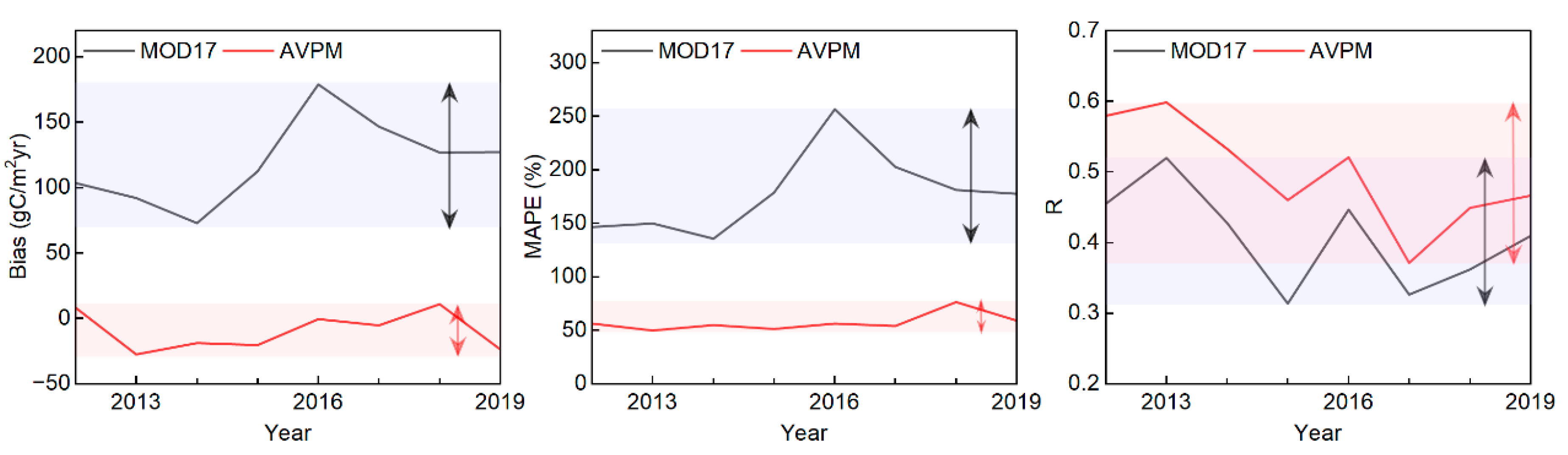
Figure 1. Location of the study area and vegetation types. Study area, including the Three-River Headwaters (TRH) region: (a) location relative to China, (b) elevation, and (c) vegetation types.
Agronomy 13 00431 g001
Figure 2. The average bias, mean absolute percentage error (MAPE), and Pearson’s correlation coefficient (r) from 2012 to 2019 for the MOD17 and AVPM. The black arrows indicate the variation range of the MOD17’s accuracy index. The red arrows indicate the variation range of the AVPM’s accuracy index.
Agronomy 13 00431 g002
Figure 3. The net primary productivity of the alpine meadow and alpine steppe from 2001 to 2020.
Agronomy 13 00431 g003
Figure 4. Distribution of the net primary productivity (NPP) and its changing trend in the Three-River Headwaters region, including (a) the average NPP from 2001 to 2020, av: alpine vegetation, as: alpine steppe, am: alpine meadow, ash: alpine shrub land; (a1) the area percentage corresponding to the eight classes in the (a); (a2) the average NPP and its one standard deviation (SD) along the longitude; (a3) the average NPP and its SD along the latitude; (b) the changing trend of NPP from 2001 to 2020; (c) the changing characteristics of the NPP from 2001 to 2020.
Agronomy 13 00431 g004
Figure 5. Patterns of minimum relative humidity ( RH min ), soil gravimetric water content (GWC), vapor pressure deficit (VPD), daytime VPD ( VPD day ), maximum VPD ( VPD max ), MOD17 water stress (mf(W)), and AVPM water stress (af(W)) during 2014–2017 at Guide station (a,c,e) and Tuotuo River station (b,d,f).
Agronomy 13 00431 g005
Table 1. Accuracy assessment of the AVPM model and MOD17 NPP from 2012 to 2019 and their bias, MAPE, and r, respectively. MAPE: mean absolute percent error; r: Pearson’s correlation coefficient; AVPM: alpine vegetation photosynthesis model.
YearBias (gCm−2yr−1)MAPE (%)rn
MOD17AVPMMOD17AVPMMOD17AVPM
2012103.38.1146.456.20.45500.5793189
201391.9−27.7149.949.70.51950.5982188
201472.7−18.8135.554.70.42740.5325194
2015112.3−20.6178.551.00.31340.4600199
2016178.8−0.7256.656.30.44660.5207199
2017146.5−5.4202.654.00.32600.3709196
2018126.810.8181.076.30.36180.4491178
2019127.1−23.6177.359.00.40910.4661184
Average120.2−9.8179.057.00.36980.48091527
Disclaimer/Publisher’s Note: The statements, opinions and data contained in all publications are solely those of the individual author(s) and contributor(s) and not of MDPI and/or the editor(s). MDPI and/or the editor(s) disclaim responsibility for any injury to people or property resulting from any ideas, methods, instructions or products referred to in the content.

