Applicability of Machine-Learned Regression Models to Estimate Internal Air Temperature and CO₂ Concentration of a Pig House

Abstract

Carbon dioxide (CO₂) emissions from the livestock industry are expected to increase. A response strategy for CO₂ emission regulations is required for pig production as this industry comprises a large proportion of the livestock industry and it is projected that per capita pork consumption will rise. A CO₂ emission response strategy can be established by accurately measuring the CO₂ concentrations in pig facilities. Here, we compared and evaluated the performance of three different machine learning (ML) models (ElasticNet, random forest regression (RFR), and support vector regression (SVR)) designed to predict CO₂ concentration and internal air temperature (T_i) values in the pig house used to regulate a heating, ventilation, and air conditioning (HVAC) control system. For each ML model, the hyperparameter was optimised and the predictive accuracy was evaluated. The order of predictive accuracy for the ML models was ElasticNet < SVR < RFR. Hence, random forest regression provided superior prediction performance. Based on the test dataset, for T_i prediction by RFR, R² ≥ 0.848 and the root mean square error (RMSE) and mean absolute error (MAE) were 0.235 °C and 0.160 °C, respectively, whilst for CO₂ concentration prediction by RFR, R² ≥ 0.885 and the RMSE and MAE were 64.39 ppm and ≤ 46.17 ppm, respectively.

1. Introduction

Concern about global warming and climate change is increasing worldwide as the concentrations of greenhouse gases (GHG) such as carbon dioxide (CO₂) and methane (CH₄) continue to rise in the atmosphere. GHGs in general and CO₂ in particular are the main causes of climate change [1,2,3,4]. Studies on carbon neutrality and the transition from fossil fuels to renewable energy sources are ongoing [5]. Nevertheless, the Energy Information Administration (EIA) predicted that global energy-usage-related CO₂ emissions will steadily increase through to 2050 (EIA, 2021). Both OECD (Organisation for Economic Co-operation and Development) and non-OECD countries are expected to increase carbon emissions. In non-OECD and OECD member nations, carbon emissions are expected to increase by 35% and 5%, respectively, relative to 2020 levels [6].

The Republic of Korea is an OECD member with a mandate to reduce GHG emissions. As of 2019, they had reached 701.37 million tons CO₂-eq. The GHG emissions from energy, industrial process, and agriculture were 611.5, 51.99, and 20.96 million tons of CO₂-eq, respectively [7]. Though the agriculture sector was responsible for only 2.9% of the total GHG emissions, the livestock sector alone accounted for nearly half the total agricultural emissions (8.6 million tons CO₂-eq). Agricultural CO₂ emissions are expected to rise in response to increases in livestock product consumption and the number of rearing heads of cattle and pigs. Thus, it was proposed that CO₂ emissions from the livestock sector should be mitigated through decreasing livestock numbers [8]. However, remedial measures such as low-carbon livestock management could hinder the growth of the livestock industry as they reduce the number of rearing heads and productivity. A low-carbon livestock product certification system was being developed for the livestock sector as a representative CO₂-reduction project in the effort to meet carbon neutrality demands. CO₂ sampling, separation, transport, storage, and utilisation technologies are being researched and developed to reduce CO₂ emissions [9]. However, it is necessary to develop accurate carbon concentration measurement and prediction methods to enable these technologies to achieve carbon neutrality. The pig industry comprises approximately 35.3% of all livestock production [10]. According to the prospect of an increase in per capita pork consumption, a response strategy for CO₂ emission regulations is required. The strategy for responding to CO₂ emissions can first be set by accurately measuring internal CO₂ concentrations in pig houses.

The CO₂ concentrations inside pig houses have been directly measured with sensors, internal air quality and ventilation performance can be indirectly evaluated using these data. Previous studies [11,12] evaluated the air quality of the rearing environment by monitoring the CO₂ concentration in a pig house. Blanes and Pedersen (2005) [13] quantitatively analysed and validated ventilation characteristics by measuring the internal CO₂ concentration in a commercial pig house. Lee et al. (2005) [14] measured the CO₂ concentration inside a pig house and calculated the ventilation and CO₂ generation rates using a CO₂ balance equation and the measured CO₂ concentration. Most of the previous studies used the field-measured CO₂ concentrations as the input for the analysis of ventilation characteristics via the CO₂ balance equation. Before a CO₂ measurement sensor is implemented, the space and installation costs required for it must be considered. Furthermore, the sensor must be recalibrated periodically and the measurement environment must be properly managed [15]. Nevertheless, missing data and outliers always occur as a consequence of sensor, communication, and server computer failure. Other researchers [16,17] evaluated the thermal, gas distribution, and internal ventilation rates in livestock facilities using the CO₂ tracer gas decay (TGD) method and computational fluid dynamics (CFD). CFD can variously set the initial boundary conditions, including gas concentration and environmental factors, according to user requirements. Though CFD can run various analyses on vast amounts of data, it nonetheless demands substantial calculation time and computing power.

Recently, several studies have been conducted in the attempt to automate the control of the optimal internal environment based on information and communications technology (ICT) convergences, such as smart farms including smart livestock and smart greenhouses. Until now, machine learning (ML)-related research in the livestock sector has focused mainly on predicting basic environmental parameters and animal growth rates, as well as identifying individuals affected by disease. To these ends, prior studies used environmental and image data. However, predictions of the internal air temperature (T_i) and the internal CO₂ concentration are needed to maintain the rearing environment of pig farms and calculate their carbon emissions, respectively. A previous study [18] estimated CO₂ emissions by analysing the factors influencing the changes in field-measured concentrations of CO₂ generated by the manure in mechanically ventilated pig houses. A statistical model was developed to estimate CO₂ emissions based on pig weight, ventilation rate, and manure temperature. These variables are closely related to CO₂ generation. Zong et al. (2014) [19] used field-measured data to develop a statistical model estimating the amount of CO₂ generated in fattening pig houses fitted with partial pit ventilation systems. Nevertheless, certain traditional statistical models fail to meet complex hypothesis conditions and strict data requirements. By contrast, ML models are not generally required to meet these criteria and may be continuously revised to accommodate new data. However, few studies have developed or evaluated ML models that can estimate CO₂ concentrations and T_i in pig houses. Arulmozhi et al. (2022) [20] attempted to estimate T_i but did not integrate the environment control devices or pig characteristics into the ML model. A control algorithm based on the predicted CO₂ concentration can prevent sudden increases in CO₂ concentration and reduce energy consumption by driving a low-power exhaust fan. Carbon neutrality can be applied, and productivity can be increased by implementing ML models that predict CO₂ concentrations using essential environmental variables in livestock production and by assessing the prediction performance of these models.

In the present work, the performance of three ML models at predicting the internal CO₂ concentration and the T_i of an experimental pig house was analysed and compared. First, the data generated during the experimental period was pre-processed by removing redundant values and outliers and through normalisation. The entire dataset was divided into training (80%) and test (20%) subsets. Each ML model [ElasticNet, random forest regression (RFR), and support vector regression (SVR)], to predict the pig house T_i and the internal CO₂ concentration, was designed. Finally, the hyperparameter was optimised and the prediction accuracy of each ML model was evaluated.

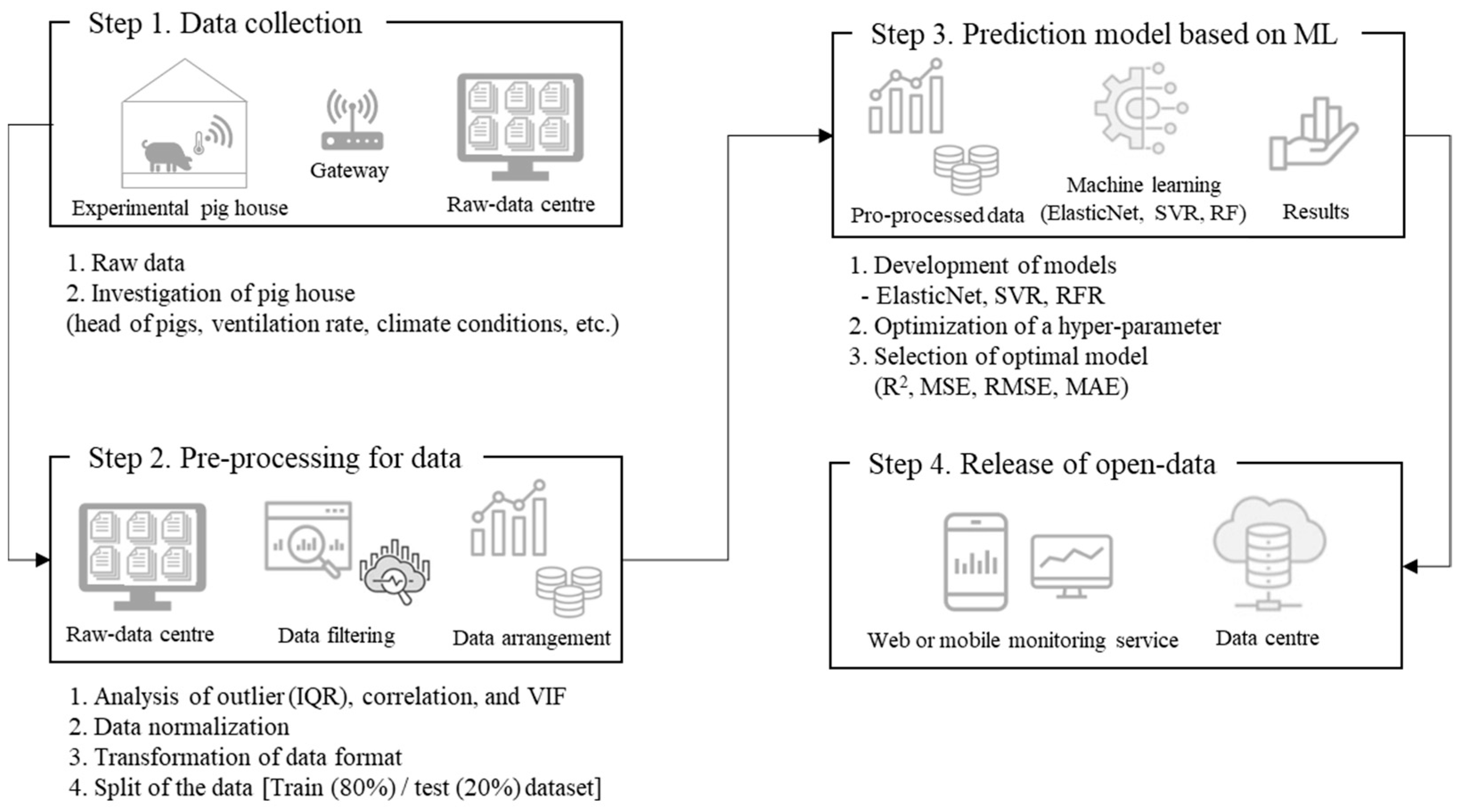
2. Materials and Methods

Figure 1 shows a detailed flowchart of the present study. The machine learning (ML) models were developed using environmental data measured inside and outside the pig house and applied to predict the T_i and internal CO₂ concentration. The predictive performance of each ML model was evaluated. The internal and external environmental data (independent variables; features) of the pig house included solar radiation, internal and external air temperature (T_e), relative humidity (RH), exhaust fan operating rate, and pig weight and heat generation. The predictive data (dependent variables; labels) included T_i and internal CO₂ concentration. The ElasticNet, SVR, and RFR ML models were used to predict pig house T_i and internal CO₂ concentration. Collaboration/Scikit-learn (https://github.com/scikit-learn/scikit-learn) was used to develop the prediction models. The hyperparameter for each ML model was optimised. The predictive accuracies of the ML models were validated using the determination coefficient (R²), the mean absolute error (MAE), and the root mean square error (RMSE).

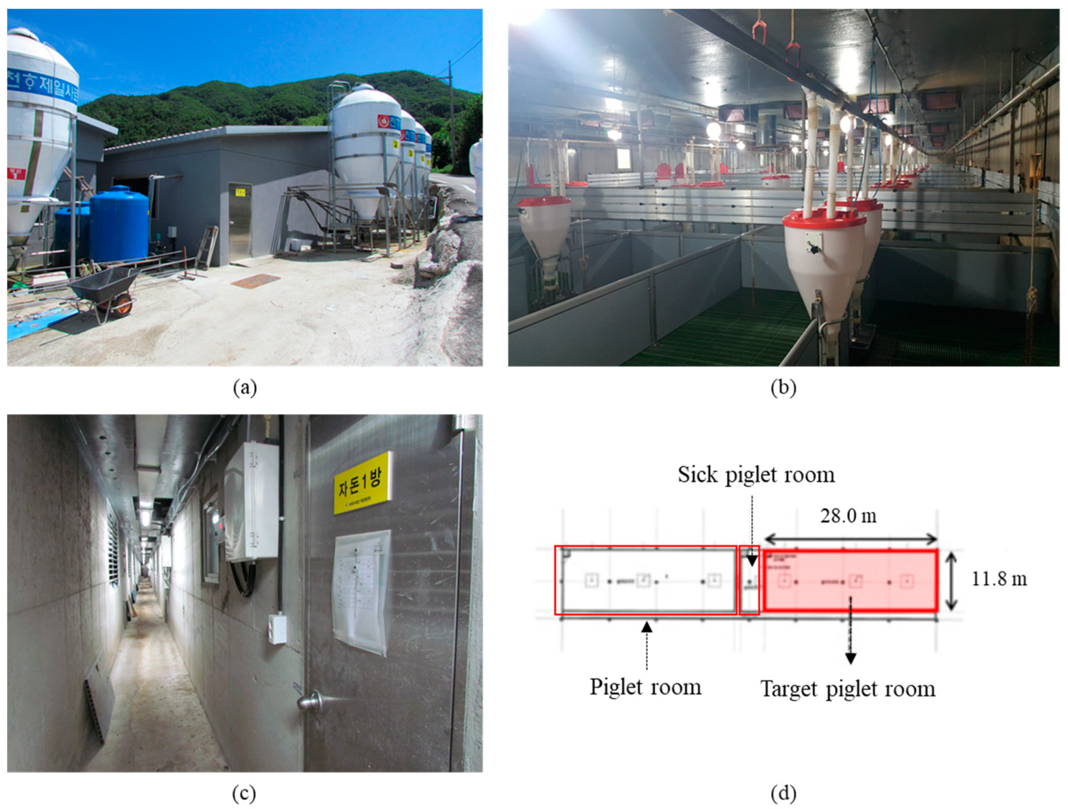
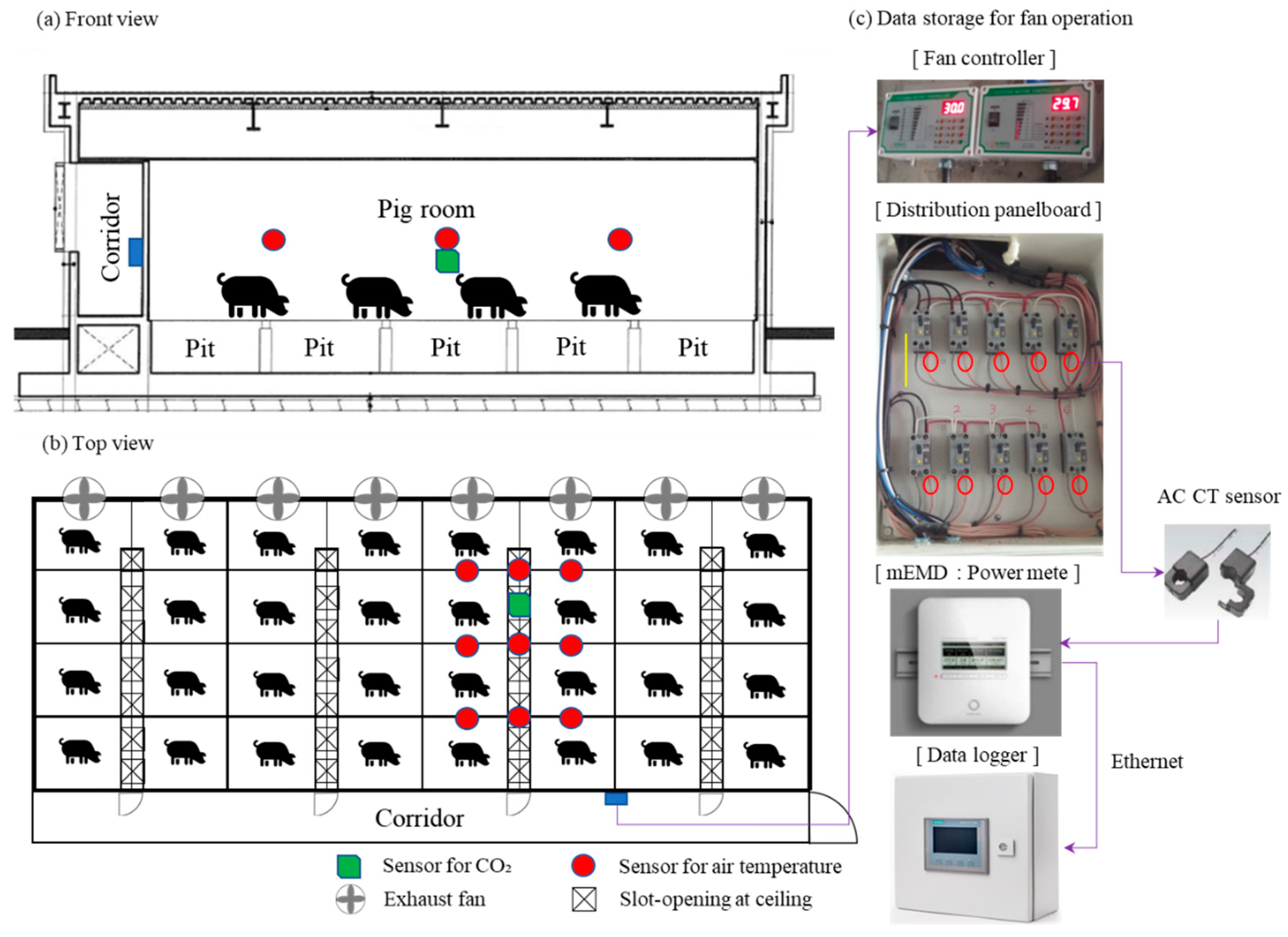
2.1. Training Data (Experimental Pig House and Breeding Conditions)

Field experiments were conducted between 1 and 28 July 2020 to predict the T_i and internal CO₂ concentration of the experimental pig house. The pig farm was located in Suncheon (35.81905° N, 127.733° E), Republic of Korea. The pig house consisted of three rooms for healthy and sick piglets (Figure 2). The worker passageway floor was made of concrete and the piglet rearing space floor consisted of plastic slats. About 900 piglets were raised in each pig room for 10 weeks and the piglet weight gain was 25 kg. The internal thermal environment of the pig house was set and maintained at 28 °C with an exhaust fan (SL-300; Sung-il Co., Seoul, Korea). Each pig room contained four roof exhaust fans (D 500 mm; 8500 m³ h⁻¹ (CMH); 418 W) and six sidewall exhaust fans (D 500 mm; 8500 CMH; 535 W). The ventilation system ran continuously to regulate the air temperature in the pig house and remove pollutants and humidity from it. One piglet room was designated as a field experiment space. The air temperature (PR-20; OMEGA Engineering Inc., Norwalk, CT, USA), CO₂ concentration (SH-VR260; SOHA Tech Co., Ltd, Seoul, Korea), and exhaust fan operating rate (mEMD; GreenENS Co., Ltd., Gwangju, Korea) were monitored in real time. Figure 3 shows the sensor installations in the pig house. All sensor nodes were installed 1.0 m above the pit floor.

Table 1. Experimental pig house and rearing data.

Pig House Type	Mechanically Ventilated Pig House	Floor Area and Volume	330.4 m2 1387.7 m3
Floor type	Partially concreted	Number of exhaust fans	Roof	4
			Sidewall	6
Number of piglet growth days	50–90	Fan size and performance	Roof	D500/8500CMH (418 W)
			Sidewall	D500/8500CMH (535 W)
Cleaning pig house and pit	Before bringing in new piglets	Set ventilation controller air temperature	28 °C

lists the specifications of the experimental pig house.

2.2. Machine Learning Model

ElasticNet, SVR, and RFR were used as regression-based ML models and Python v. 3.10 (https://www.python.org/downloads/release/python-3100/, accessed on 17 May 2022) was used to develop them. Python is a free open-source programming language that can incorporate and run modules created in other programming languages. Furthermore, Python requires no compilation and can be coded at the same time that its output is being checked. Scikit-learn (https://github.com/scikit-learn/scikit-learn, accessed on 17 May 2022) was used as a library for the ML models. Pandas (https://pandas.pydata.org, accessed on 17 May 2022), NumPy (https://numpy.org/install, accessed on 17 May 2022), and others were used as data processing libraries.

2.2.1. ElasticNet

Simple linear regression models predict one dependent variable by using one independent variable. In contrast, multiple linear regression models predict one dependent variable by using several independent variables. The least square method is used to obtain the regression coefficient in linear regression analysis (Equation (1)). Linear regression minimises mean square error (MSE). Increasing the number of independent variables can lead to multicollinearity. On the other hand, decreasing the number of independent variables may constrain model optimisation.

$$\mathrm{y}={\mathsf{\beta }}_0+{\beta }_1{x}_1+{\beta }_2{x}_2+\cdots +{\beta }_n{x}_n+\mathsf{\epsilon }$$

(1)

where $\mathrm{y}$ is the dependent variable (label), $x_i$ is the independent variable (feature (1 to n)), ${\mathsf{\beta }}_i$ is the regression coefficient used to predict $\mathrm{y}$ (1 to n), ${\mathsf{\beta }}_0$ is the model intercept/constant, and ε is the model noise or random error.

The last absolute shrinkage and selection operator (LASSO) and Ridge were developed to overcome the shortcomings of linear regression and improve its versatility. In LASSO regression, important variables are selected using hyperparameters (α and L1-ratio) whilst other variables are excluded from the regression equation by setting the regression coefficient to zero. In Ridge regression, the regression coefficient is reduced using α. For this reason, the regression coefficient may significantly fluctuate with α value. Thus, ElastiNet combines L1-regulation (LASSO) with L2-regulation (Ridge) to attenuate the dependence of the regression coefficient on α [21,22]. In ElasticNet, LASSO selects variables whilst Ridge mitigates multicollinearity.

$$\mathrm{J}{\left(\mathsf{\theta }\right)}_{Lasso}=\frac{1}{n}{\displaystyle \sum }_{i=1}^n{\left(y_i-{\widehat{y}}_i\right)}^2+\lambda {\displaystyle \sum }_{j=1}^m\left|{\omega }_j\right|$$

(2)

$$\mathrm{J}{\left(\mathsf{\theta }\right)}_{Ridge}=\frac{1}{n}{\displaystyle \sum }_{i=1}^n{\left(y_i-{\widehat{y}}_i\right)}^2+\lambda {\displaystyle \sum }_{j=1}^m{\omega }_j{}^2$$

(3)

$$\mathrm{J}{\left(\mathsf{\theta }\right)}_{ElasticNet}=\frac{1}{n}{\displaystyle \sum }_{i=1}^n{\left(y_i-{\widehat{y}}_i\right)}^2+\mathsf{\gamma }\lambda {\displaystyle \sum }_{i=1}^n\left|{\omega }_i\right|+\frac{1-\gamma }{2}\lambda {\displaystyle \sum }_{i=1}^n{\omega }_i^2$$

(4)

where $\frac{1}{n}{{\displaystyle \sum }}_{i=1}^n{\left(y_i-{\widehat{y}}_i\right)}^2$ is the mean square error (loss function), $\lambda {{\displaystyle \sum }}_{j=1}^m{\omega }_j{}^2$ is the Ridge penalty (L2-regulation), $\lambda {{\displaystyle \sum }}_{j=1}^m\left|{\omega }_j\right|$ is the LASSO penalty (L1-regulation), $\mathsf{\gamma }\lambda {{\displaystyle \sum }}_{i=1}^n\left|{\omega }_i\right|$ is the L1-regulation ElasticNet penalty, and $\frac{1-\gamma }{2}\lambda {{\displaystyle \sum }}_{i=1}^n{\omega }_i^2$ is the L2-regulation ElasticNet penalty.

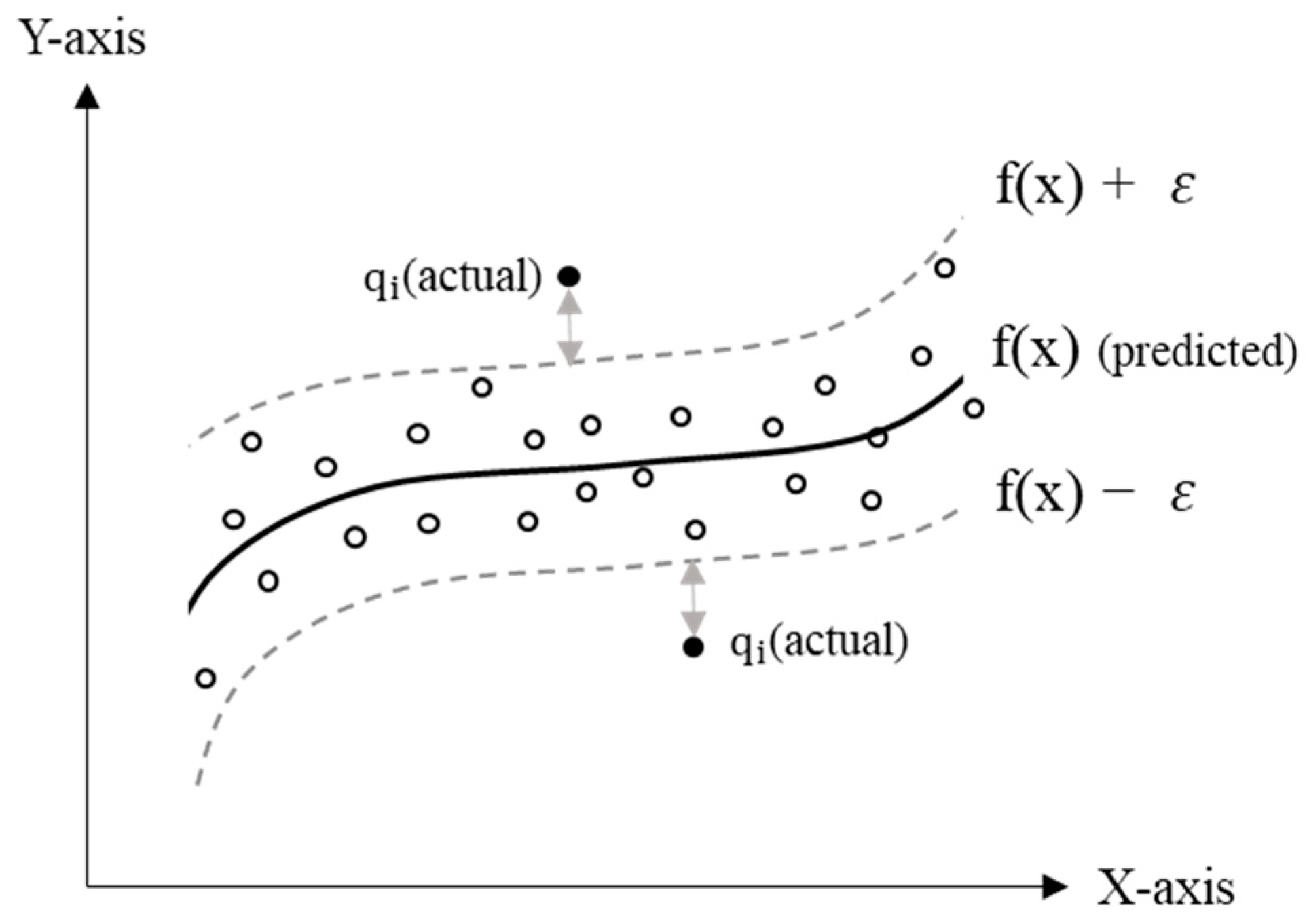
2.2.2. Support Vector Regression (SVR)

The ML method known as support vector machine (SVM) is a supervised learning model that analyses data. It is used mainly in classification and regression analysis. Support vector regression (SVR) applies an ε-insensitive loss function to SVM and extends its use in regression analysis [23]. SVR maintains the difference between the actual and predicted values within ε (Figure 4). ε is an error tolerance and the kernel function increases the dimensions to design a regression model that can accurately solve even nonlinear problems. Whereas artificial neural networks (ANN) require abundant training data, SVR can generate accurate results even with minimal training data.

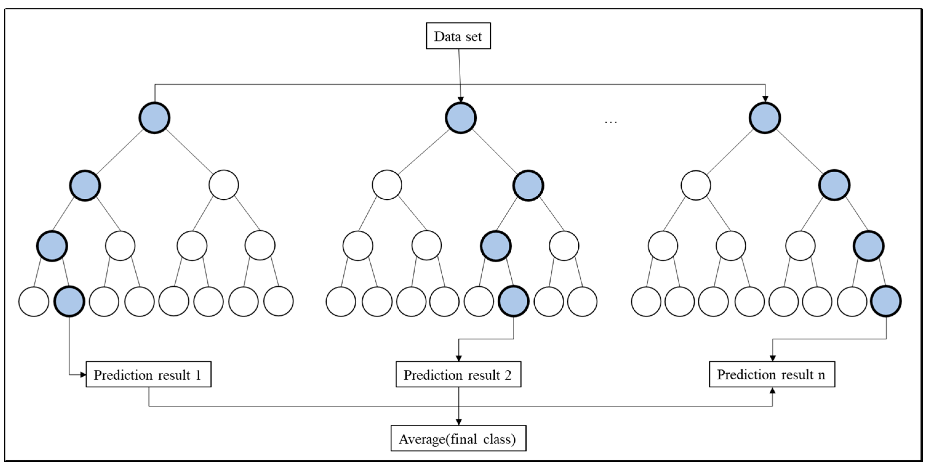
2.2.3. Random Forest

The random forest (RF) model is suitable both for regression analysis and classification. RF generates decision trees by randomly sampling data from a dataset via the Bagging (bootstrap aggregation) technique. RF is created by combining the prediction results of each decision tree into a single model [24]. Figure 5 shows that when the dataset is entered as the input, the output is calculated as the prediction results. An ensemble technique that averages and collects the output of each regression tree lowers the risk of model overfitting. Prediction quality improves with the number of decision trees generated in the RFR model. On the other hand, the amount of space required for analysis and the performance level required for the computer conducting the analysis also increase with the number of decision trees generated.

2.3. Data Pre-Processing and Training

The independent variables (features) strongly influence the accuracy of the ML prediction model [25]. For this reason, the appropriate independent variables should be selected to predict the pig house T_i and internal CO₂ concentration. Independent variables that are highly correlated with the dependent variables (labels) should be selected. This process is called feature selection. Moreover, data training under various scenarios is essential. Environmental data for the experimental pig house (solar radiation, wind speed, internal and external air temperature, RH, pig body weight, and growing day) were collected between 1 and 28 July 2020.

High-quality data must be extracted and analysed to build an optimal training dataset. Data pre-processing was conducted for this purpose. The N/A value (uncollected data) generated from monitoring device self-inspection and error was deleted. Outliers were also subjected to data pre-processing by analysing outside the quartile range (IQR). If the data range was too wide, then noise data could be generated or overfitted. Hence, normalisation was performed to prevent these errors and accelerate training [26].

$$X_{normalised}=\frac{X-X_{min}}{X_{max}-X_{min}}$$

(5)

where $X_{normalised}$ is the normalised value, $X$ is the data point, $X_{min}$ is the minimum value of any variable, $X_{max}$ is the maximum value of any variable, and $\overline{y}$ is the average of the field-measured data.

ML models have hyperparameters that must be determined to ensure precise and reliable model operation. In fact, model performance may significantly vary with the degree of control of the hyperparameters. Determination of the hyperparameter range and interval setting may depend upon developer experience [27]. ElasticNet was designed by combining the proportions of the L1- and L2-regulations or the L1-ratio. As the regression model regulation method requires manual adjustment of the α value, α was set to 0.02, 0.05, and 0.1, whilst the L1-ratio (L1-regulation weight; 0 < L1 ratio < 1) was set to 0.25, 0.5, and 0.75. The commonly applied radial basis function (RBF) kernel function was used for the SVR model. C and γ selection of the RBF kernel function directly affect SVR model accuracy and generalisation ability [28]. γ determines the curvature of the model boundary whilst C determines the extent to which the data samples may be placed in different classes. To ensure good SVR model performance, it is necessary to adjust C (smooth decision boundary factor) and γ to the model complexity. Algorithm complexity increases with C and γ. C and γ were set to 0.01, 0.1, 1, 10, and 100 to estimate the RBF kernel function hyperparameters. The number of trees (n-estimators) was set to 1, 10, 50, and 100 to optimise the RFR hyperparameters.

Table 2. Hyperparameters for ML models.

Algorithm	Hyperparameter	Defined Values
ElasticNet	α	0.02, 0.05, and 0.1
	L1 ratio	0.25, 0.5, and 0.75
SVR	C	0.01, 0.1, 1, 10, and 100
	γ	0.01, 0.1, 1, 10, and 100
RF	n-estimator	1, 10, 50, and 100

lists the hyperparameter conditions for each ML model.

The amount of data may be increased to enhance the predictive performance of the model. Nevertheless, the appropriate training to test dataset size ratio must be selected. The data were divided into training (80%) and test (20%) datasets to predict the pig house T_i and internal CO₂ concentration.

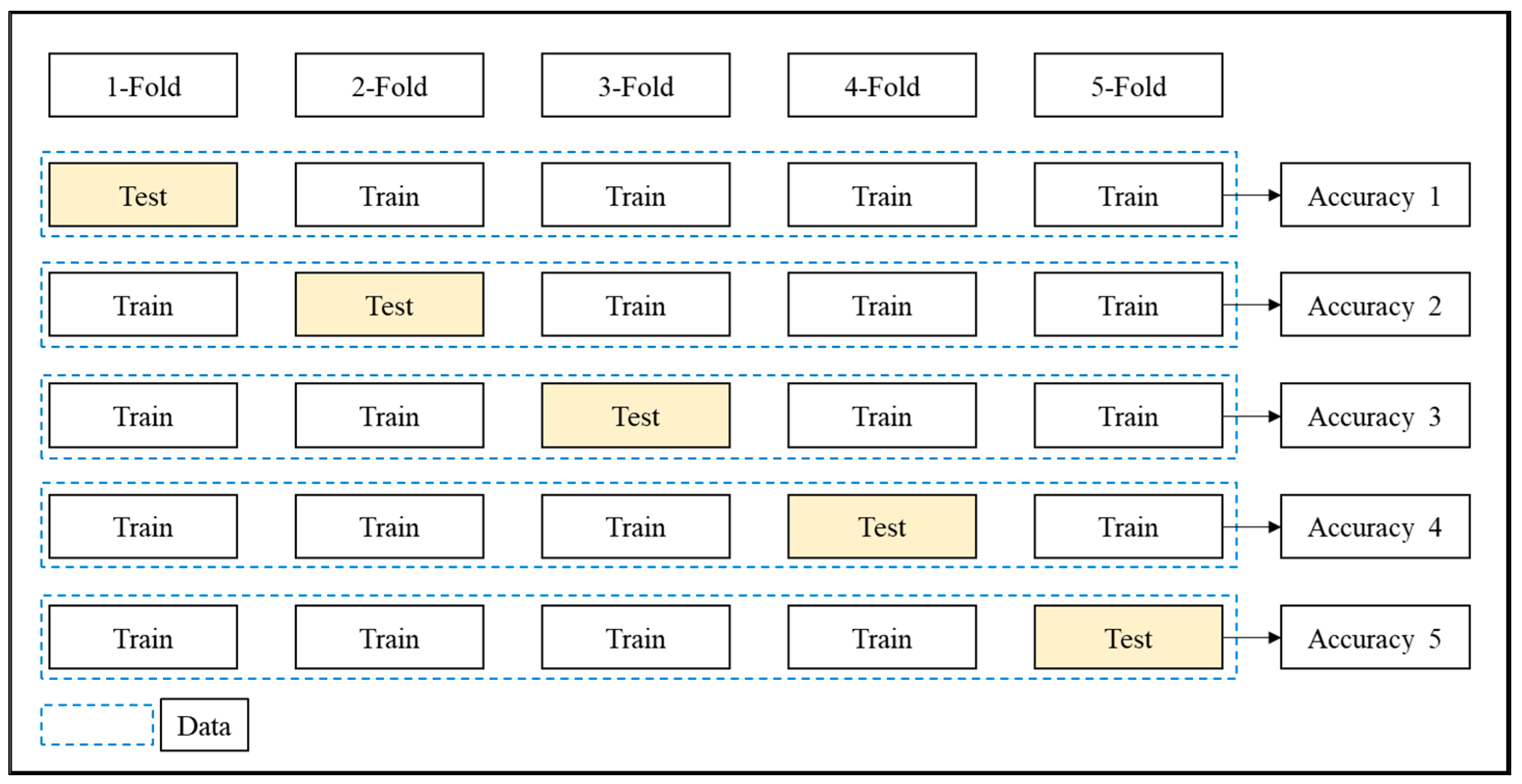
2.4. Predictive Model Validation and Selection

Each ML model was validated by comparing the T_i and internal CO₂ concentration data that it predicted against the field-measured T_i and internal CO₂ concentration data. Twenty percent of the total data for the experimental period was subjected to k-Fold cross-validation. In the latter procedure, the training dataset has k groups of the same size that are designated as Folds. The k-Folds consist of (k-1) training folds and one test fold that are validated k times (Figure 6). In the present study, pig house air temperature and internal CO₂ concentration were predicted using an experimental dataset.

R², RMSE, and MAE are used to evaluate the performance of models at predicting specific environmental variables. Statistical indicators such as R² and MSE that are calculated by using squared data are difficult to understand intuitively as they have different dimensions. Hence, MAE was also analysed as it indicates the average error magnitude by applying absolute values. MAE determines the quantitative error between the actual and predicted values. MSE is a squared average of the difference (error) between the observed and predicted values. As it obtains the square of the error, its value is larger than the actual average error. Compared with MSE, RMSE more comprehensively penalises large errors. MAE is a statistical error indicator that is the average of the absolute value (predicted value minus observed value). MAE is calculated as shown in Equation (9):

$$R^2=\left[\frac{{{\displaystyle \sum }}_{i=1}^n\left(y_i-\overline{y}\right)\left({\widehat{y}}_i-\tilde{y}\right)}{\sqrt{{{\displaystyle \sum }}_{i=1}^n{\left(y_i-\overline{y}\right)}^2{{\displaystyle \sum }}_{i=1}^n{(\widehat{y_i}-\tilde{y})}^2}}\right]$$

(6)

$$MSE=\frac{{{\displaystyle \sum }}_{i=1}^n{\left(y_i-{\widehat{y}}_i\right)}^2}{n}$$

(7)

$$RMSE=\sqrt{MSE}$$

(8)

$$MAE=\frac{1}{n}{\displaystyle \sum }_{i=1}^n\left|y_i-{\widehat{y}}_i\right|$$

(9)

where n is the total number of data points, $y_i$ are field-measured data, $\overline{y}$ is the average of the field-measured data, ${\widehat{y}}_i$ are the ML-based predicted data, $\tilde{y}$ is the average of the ML-based predicted data, R² is the coefficient of determination, MSE is the mean square error, RMSE is the root mean square error, and MAE is the average value of all absolute errors.

3. Results and Discussion

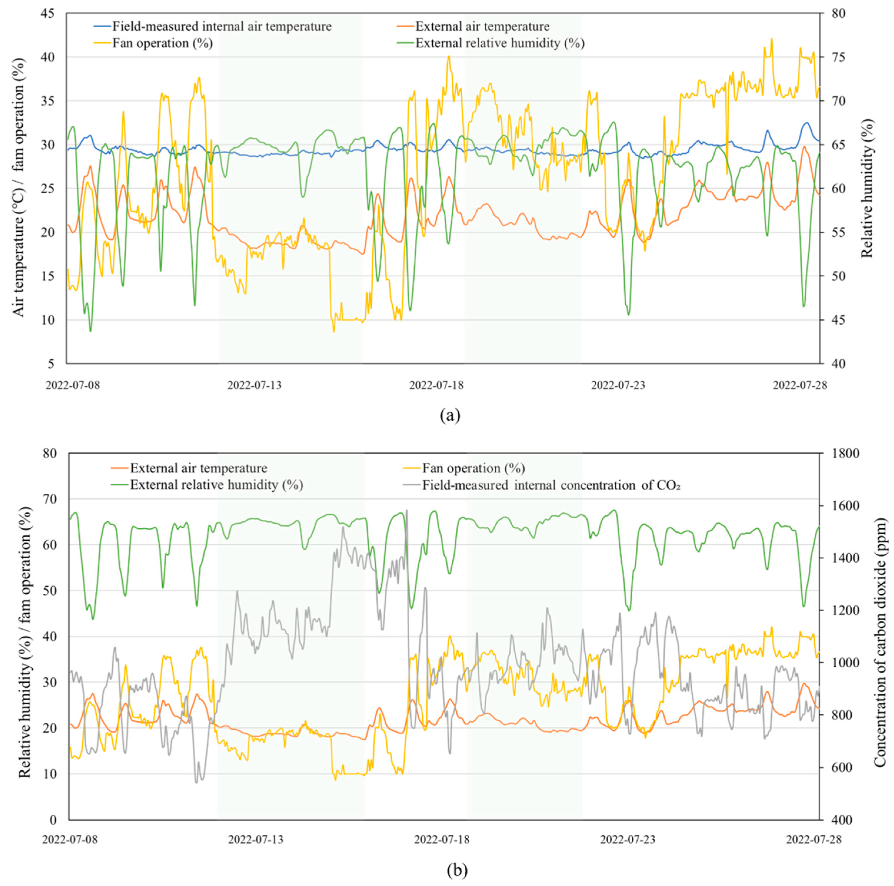
3.1. Field-Measured Experimental Pig House Data

The rearing environment (air quality) greatly affects pig productivity. Hence, proper environmental air quality control is needed. In particular, air temperature and CO₂ concentration are correlated with feed intake, water consumption, and internal humidity. Figure 7 shows the data for the external and internal environment and environmental control device operation of the pig house measured during the field experiment. The pig house T_i was in the range of 28.4–32.5 °C. The average pig house air temperature was 29.4 °C and T_i was maintained at 2.4–6.5 °C above the optimal (26 °C). Although it was early summer, the internal thermal environment was controlled to lower energy costs and the risk of respiratory diseases. Relative humidity (RH) was high between 12 and 16 July 2022 and between 19 and 22 July 2022 as the weather was cloudy and T_e was reduced (Figure 7). During the other experimental periods, T_e rose immediately after sunrise and the fan operated at a higher rate. These results were consistent with the environmental data characteristic of sunny days. The internal RH of the pig house was measured to maintain the appropriate RH range, namely, 50−70% [29]. When T_e was low, the exhaust fan operated at a variable rate. When T_e was high, the pig house T_i increased even though the exhaust fan operated at a higher rate.

The average, minimum, and maximum CO₂ concentrations in the pig house were 986.3 ppm, 541.8 ppm, and 1570.8 ppm, respectively. The CO₂ concentration was at its minimum when the exhaust fan operated at a high rate. By contrast, when the exhaust fan operated at a low rate, the CO₂ accumulated and neared its maximum concentration in the pig house. On certain days, the internal CO₂ concentration exceeded 1000 ppm which corresponds to the previously reported CO₂ concentration limit [30]. The logic control of the exhaust fan in the pig house operated according to the pig house T_i. If the operating rate of the exhaust fan was maintained at ≥30%, the internal CO₂ concentration in the pig house could be maintained at a level ensuring the appropriate rearing environment. An earlier study [31] analysed the impact of the ventilation rate on changes in the internal gaseous pollutant concentrations in a closed pig house. The total suspended particulate (TSP) concentration did not significantly vary with ventilation rate (p > 0.05). However, the pollutant concentrations decreased with increasing ventilation rate.

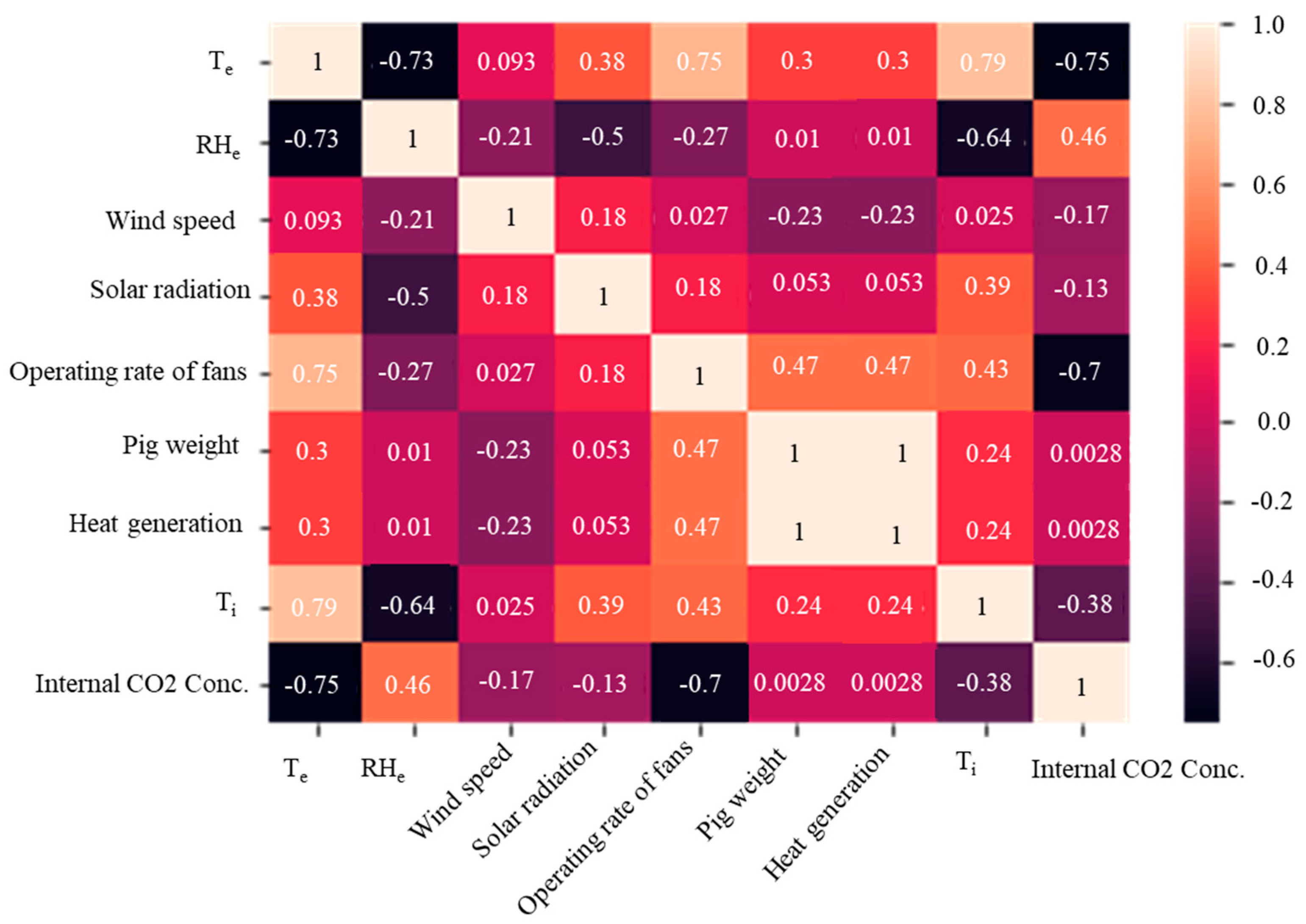
3.2. Selection of Machine Learning (ML) Model Features

In feature selection, independent variables are chosen to construct the ML model. ML model complexity increases with the number of model features. Hence, the use of excess model features increases the risk of overfitting. Feature selection reduced model complexity whilst improving performance and increasing processing speed. Pearson’s correlation coefficient analysis was conducted to select the ML model features used herein. Figure 8 shows the Pearson’s coefficients of correlation (R) between variables measured in the experimental pig house. Features weakly correlated (R < 0.4 or R > −0.4) with the dependent variables (T_i and internal CO₂ concentration) were eliminated to reduce redundancy and accelerate the learning model. The correlations (R) between T_e and T_i, CO₂ concentration, exhaust fan operating rate, and RH were 0.7895, −0.7537, 0.7477, and −0.7311, respectively. The external air temperature of the pig house affected the T_i, CO₂ concentration, exhaust fan operation rate, and RH. The internal CO₂ concentration was negatively correlated (R = −0.382) with the T_i of the pig house. The correlations between the exhaust fan operating rate, the internal CO₂ concentration, and the T_i of the pig house were −0.7043 and 0.43, respectively. Hence, fresh air exchange decreased whilst internal CO₂ concentration increased with exhaust fan operating rate. However, the T_i-based exhaust fans operated continuously, and the internal CO₂ concentration fluctuated. On the other hand, the exhaust fans maintained a relatively constant T_i (28−32 °C) and their operating rates were more strongly correlated with T_e than T_i.

T_e was most strongly correlated with T_i and CO₂ concentration whereas solar radiation, heat generation, and live pig weight were not significantly correlated with the carbon dioxide content. Therefore, pig house T_e, RH, and exhaust fan operating rate were the features selected for the ML models. Only the data for external air temperature, RH, and exhaust fan operating rate were trained. These data are relatively easy to acquire for pig houses and are generally applicable to ML models used in the livestock industry. As few farms install their own weather stations, it is impractical to monitor the external wind environment and radiation in real time. Based on the principal feature analysis, then, the three aforementioned features served as the input for ML models predicting T_i and internal CO₂ concentration.

3.3. Evaluation of Predictive Models

ML models were developed to predict T_i and internal CO₂ concentration in a mechanically ventilated pig house.

Table 3. T_i prediction accuracy of optimised machine learning models (ElasticNet, SVR, and RFR).

Dataset	Statistical Index	ElasticNet (a: 0.02; L1-Ratio: 0.25)	SVR (C:10 and γ: 1)	RFR (n-Estimator: 100)
Training	RMSE	0.228	0.084	0.152
	MAE	0.167	0.060	0.063
	R2	0.867	0.983	0.940
Test	RMSE	0.251	0.221	0.201
	MAE	0.178	0.151	0.141
	R2	0.835	0.865	0.891

and

Table 4. Internal CO₂ concentration prediction accuracy of optimised machine learning models (ElasticNet, SVR, and RFR).

Dataset	Statistical Index	ElasticNet (a: 0.02; L1-Ratio: 0.75)	SVR (C:100 and γ: 1)	RFR (n-Estimator: 50)
Training	RMSE	73.871	61.189	22.175
	MAE	57.995	43.668	15.632
	R2	0.853	0.899	0.987
Test	RMSE	79.702	66.415	59.468
	MAE	62.284	50.422	42.756
	R2	0.825	0.880	0.900

summarise the results of analyses validating the accuracy of the models at predicting T_i and internal CO₂ concentration. Evaluation of the accuracy of prediction of the ML model using the test dataset revealed that R², RMSE, and MAE were lower than the corresponding values in the training dataset. For ElasticNet, the accuracy of T_i prediction was higher for the test than the training dataset in terms of MAE (6.2%) and RMSE (9.2%) but lower in terms of R² (3.8%). For SVR, the accuracy of T_i prediction was higher for the test than the training dataset in terms of MAE (60.3%) and RMSE (62.0%) but lower in terms of R² (13.6%). For RFR, the accuracy of T_i prediction was higher for the test than the training dataset in terms of MAE (55.3%) and RMSE (24.4%) but lower in terms of R² (5.5%). The R² for each ML model had T_i prediction accuracy ≥ 0.83. RMSE was < 0.251 °C and MAE were 0.178 °C, 0.151 °C, and 0.141 °C for ElasticNet, SVR, and RFR, respectively. Hence, RFR had the highest T_i prediction performance. RMSE and MAE were both 0.03 °C lower for the ElasticNet model than the RFR model and their R² differed by 3.5%. There was no significant error in the air temperature prediction by any model.

The results of the model predictions for internal CO₂ concentration were similar to those for T_i when the test dataset was used. For ElasticNet, the accuracy of internal CO₂ concentration prediction was higher for the test than the training dataset in terms of MAE (6.9%) and RMSE (7.3%) but lower in terms of R² (3.4%). For SVR, the accuracy of internal CO₂ concentration prediction was higher for the test than the training dataset in terms of MAE (13.4%) and RMSE (7.9%) but lower in terms of R² (2.2%). For RFR, the accuracy of internal CO₂ concentration prediction was higher for the test than the training dataset in terms of MAE (63.4%) and RMSE (62.7%) but lower in terms of R² (9.7%). The R² for each ML model had internal CO₂ concentration prediction accuracy ≥ 0.825.

The average RMSE for ElasticNet, SVR, and RFR were 79.702 ppm, 66.415 ppm, and 59.468 ppm, respectively. Hence, this trend was the same as that for T_i prediction. The average MAE for ElasticNet, SVR, and RFR were 62.284 ppm, 50.442 ppm, and 42.756 ppm, respectively. Here, RFR also demonstrated excellent internal CO₂ concentration prediction performance whilst that of ElasticNet was the poorest. RMSE and MAE for ElasticNet were 13.29 ppm and 11.86 ppm smaller, respectively, than those for RFR, and R² differed between models by 6.3%. The RFR model generally exhibits high prediction accuracy as numerous techniques have been applied to models estimated from multiple decision trees. A previous study [32] compared the relative performance of various ML models to predict the rate of evaporation from litter in a duck house. The RF model most accurately predicted the litter evaporation rate, possibly because it amplifies data using the Bagging technique. Thus, the RF model has relatively high prediction accuracy even when insufficient data are used. Nevertheless, the model used to predict CO₂ concentration must be improved through further learning.

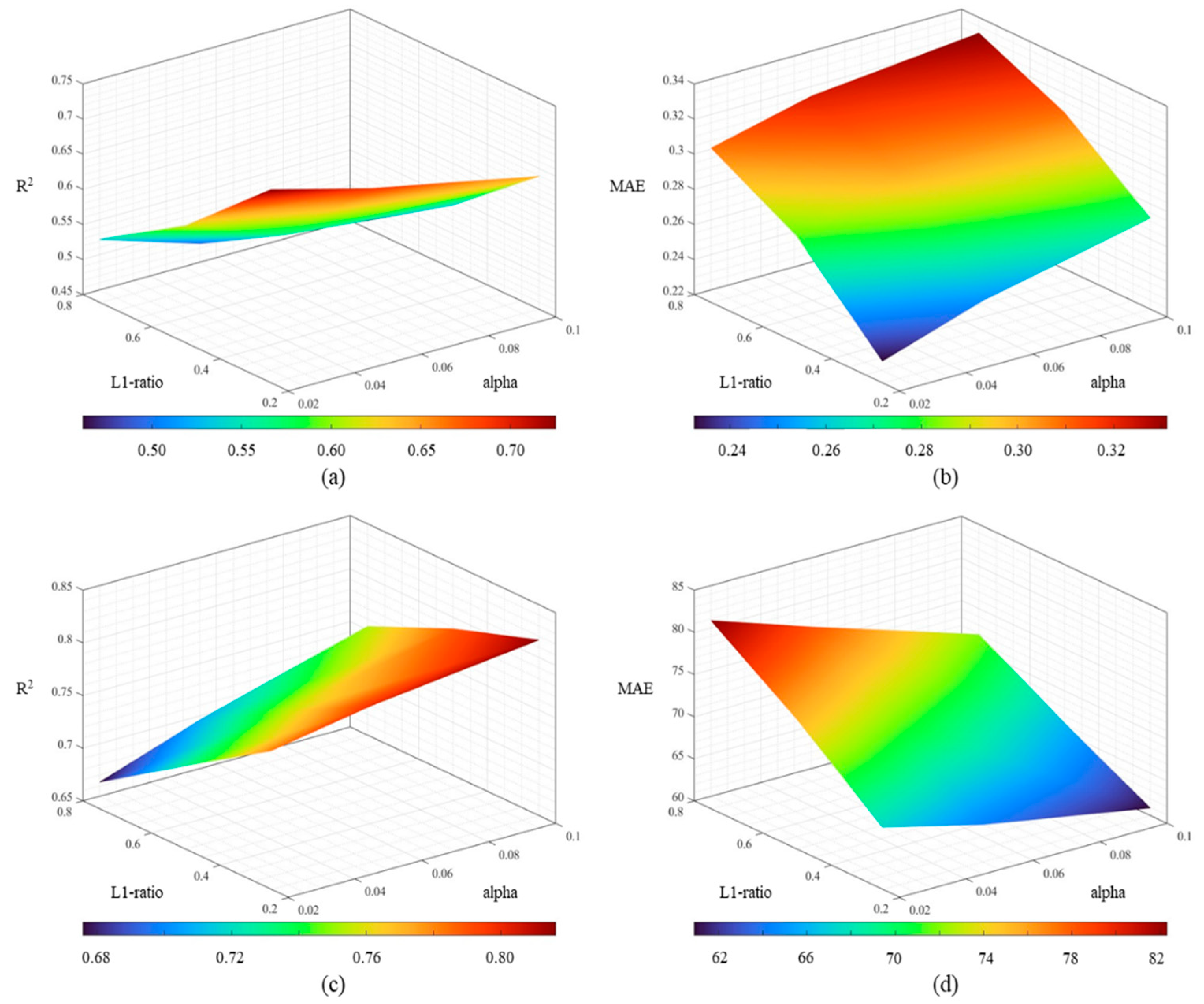
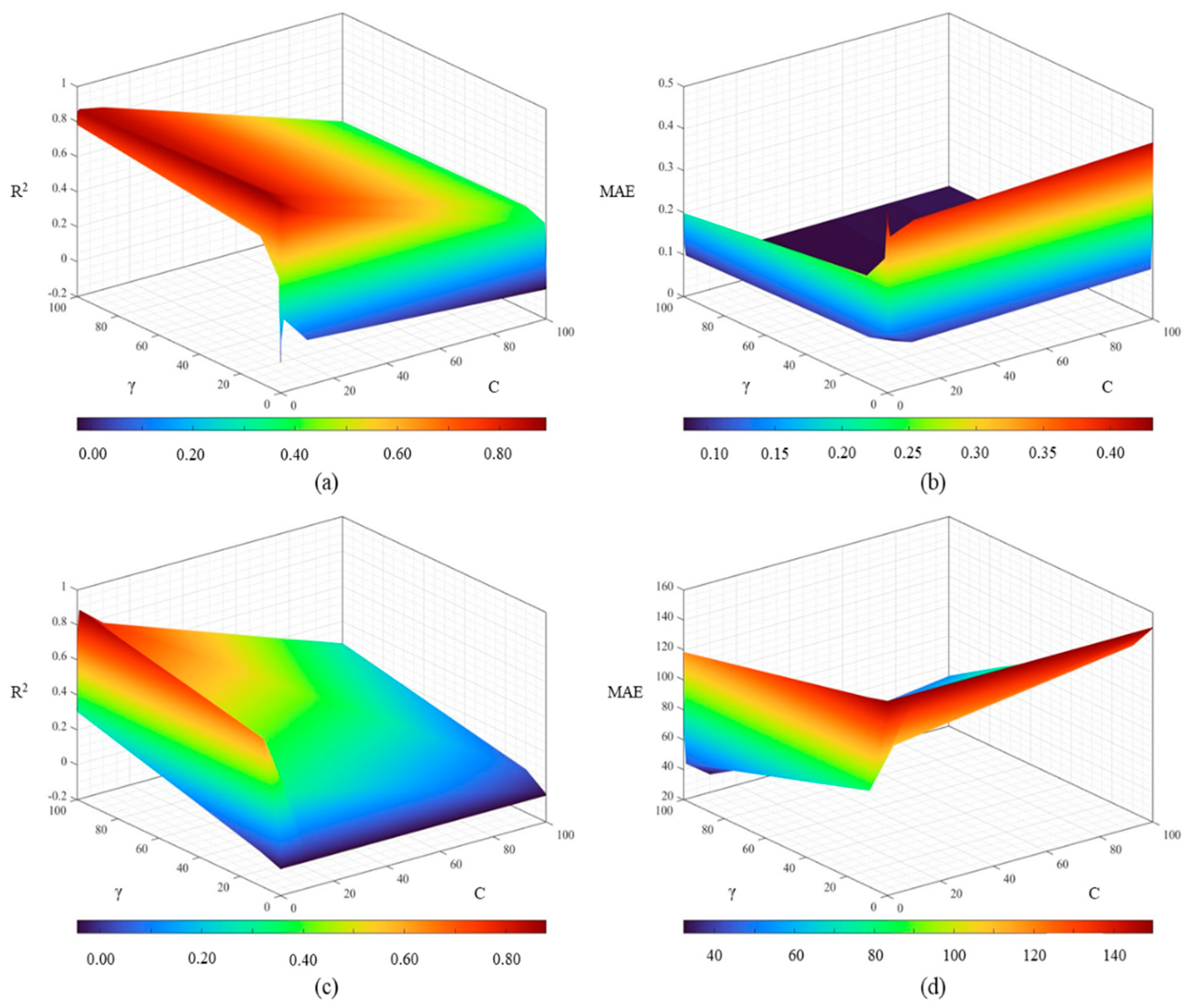
3.4. Model Evaluation by Hyperparameter Tuning

ML model parameters that must be pre-set are known as hyperparameters. Excessively large or small values can degrade model performance. Thus, hyperparameters must be carefully adjusted to optimise the performance criteria. In hyperparameter tuning, suitable parameter values for a particular dataset are found. Here, we applied a fivefold cross-validation method to find the optimal hyperparameter. We presented the prediction accuracy of non-optimised and optimised ML models to assess model performance (Figure 9 and Figure 10;

Table 5. Pig house T_i prediction accuracy of RFR model based on n-estimator.

Dataset	Statistical Index	1	10	50	100
Training	RMSE	0.184	0.1	0.265	0.265
	MAE	0.075	0.063	0.056	0.055
	R2	0.910	0.974	0.982	0.983
Test	RMSE	0.315	0.235	0.226	0.221
	MAE	0.204	0.160	0.152	0.151
	R2	0.730	0.848	0.859	0.865

and

Table 6. Pig house internal CO₂ concentration prediction accuracy of RFR model based on n-estimator.

Dataset	Statistical Index	1	10	50	100
Training	RMSE	61.013	26.978	22.175	23.458
	MAE	24.762	17.998	15.632	15.848
	R2	0.899	0.980	0.987	0.987
Test	RMSE	99.966	64.392	59.468	61.046
	MAE	63.707	46.173	42.726	43.478
	R2	0.728	0.885	0.902	0.897

).

We evaluated the ElasticNet model which considers L1- and L2-regulations. Model performance varied with L1-ratio (regulatory coefficient) and α value. In the ElasticNet model, the prediction accuracy that changed the limiting condition (α; alpha) was reduced. The average R² for predicting T_i was 0.633 when α = 0.02 and the prediction performance decreased by 31.92% (R² = 0.431) as α increased to 0.1. For the T_i prediction, RMSE = 0.524 °C when α = 0.02 and RMSE = 0.583 °C when α increased to 0.1. MAE = 0.275 °C when α = 0.02 and MAE = 0.340 °C when α increased to 0.1. Increasing the L1-ratio to 0.25, 0.5, and 0.75 decreased the average R² from 0.611 to 0.558 and increased RMSE and MAE by 12.9% (0.383–0.410 °C) and 5.81% (0.280–0.297 °C), respectively.

For ElasticNet, when α = 0.02, the average R² = 0.752 for the prediction of internal CO₂ concentration and when α increased to 0.1, R² decreased to 0.672 (10.6%). RMSE = 94.68 ppm when α = 0.02. When α increased to 0.1, RMSE increased to 108.77 ppm (32.0%). MAE = 75.138 ppm when α = 0.02 and RMSE increased to 84.707 ppm (12.7%) when α increased to 0.1. Increasing the L1-ratio from 0.25 to 0.75 increased R² from 0.708 to 0.749 and decreased RMSE and MAE by 16.2% (from 102.67 ppm to 95.25 ppm) and 6.5% (from 80.25 ppm to 75.37 ppm), respectively.

The pig house T_i and internal CO₂ concentrations were predicted using the SVR model and the hyperparameter (C and γ) values 0.01, 0.1, 1, 10, and 100 were applied to it. Figure 10 shows the T_i and CO₂ concentration prediction accuracies using the SVR model according to the hyperparameters. When γ = 1 and C = 100, SVR exhibited excellent T_i and internal CO₂ concentration prediction performance. C displayed a relatively low error rate (>1 and <100) and a relatively constant trend when the error rate was <0.1. At 0.1, 1, and 10, γ demonstrated excellent performance. When the manual search technique was applied, C and γ of 10 and 1, respectively, showed the best performance in the SVR model. When C and γ were 10 and 1, respectively, the accuracy of the SVR at predicting T_i was as follows: R² = 0.891, RMSE = 0.201 °C, and MAE = 0.141 °C. The SVR model also presented with excellent T_i prediction performance when C = 100 and γ = 1. In this case, its T_i prediction accuracy was as follows: R² = 0.877, RMSE = 0.211 °C, and MAE = 0.149 °C. The models did not significantly differ in terms of overall T_i prediction accuracy. R², RMSE, and MAE differed by 1.62%, 8.96%, and 5.41%, respectively. γ exhibited the lowest error rates at <0.01 or >100. Moreover, T_i prediction performance improved with C value. The SVR model had the highest internal CO₂ concentration prediction accuracy when C = 100 and γ = 1. In this case, R² = 0.88, RMSE = 66.42 ppm, and MAE = 50.42 ppm. The internal CO₂ concentration prediction accuracy of the SVR model increased with C value and was optimal at γ = 1.

T_i and internal CO₂ concentration prediction accuracy of the RFR model based on its n-estimator hyperparameter was evaluated. R², RMSE, and MAE values for T_i prediction by considering different n-estimators ranging from 1 to 100 were calculated. RFR model prediction accuracy increased with n-estimator value. R² had the highest value when the n-estimator was 100. For the test dataset, the accuracy of the RFR model was R² = 0.865 based on average cross-validation (Table 5). Similar results were obtained for the RFR model predictions of both internal CO₂ concentration and T_i. Table 6 shows the RFR model prediction accuracy of internal CO₂ concentration based on the n-estimator. When the n-estimator was 100, R², RMSE, and MAE had the highest values. The RFR model computational time and cost increase with the n-estimator value. Thus, there is a trade-off between RFR model performance and n-estimator value. In the present study, the predictive accuracy of the RFR model did not significantly change at n-estimator values ≥ 10. For this reason, it was determined that the optimal n-estimator value for the RFR model was 10.

4. Conclusions

It is necessary to establish a strategy responding to the regulation of CO₂ emissions from pig production. To this end, the CO₂ concentrations in pig farms must be accurately measured. To date, CO₂ emissions have been calculated based on the relationships among the internal and external CO₂ concentrations and the ventilation rate. However, poor environmental conditions constrain the collection and prediction of quantitative data by using on-site sensors. In the present study, T_i and CO₂ concentrations in an experimental pig house by using its weather and operation (environmental control device) data were predicted. Three machine learning (ML) models were designed and the accuracies of their internal air temperature and CO₂ concentration predictions were compared. The input data were processed by normalising them and eliminating redundant values and outliers before evaluating the accuracy of each ML model. Feature selection was then conducted, and three parameters were extracted and used as the model characteristics. ElasticNet, support vector regression (SVR), and random forest regression (RFR) models were applied, and their prediction performance accuracies were evaluated. The order of prediction accuracy was ElasticNet < SVR < RFR. Hence, RFR provided superior prediction performance. Model performance could be improved through hyperparameter optimisation. Analyses of the performance of each ML model in the accurate prediction of pig house T_i and CO₂ concentration could serve to develop air temperature and carbon-dioxide-based control strategies. A prior study [33] monitored CO₂ concentration-based ventilation control systems for one year and reported that they reduced overall energy consumption by 33% compared to conventional ventilation control systems. Therefore, the results of the present work provide data and reference for developing and optimising control algorithms in the future. Furthermore, the prediction of internal CO₂ concentration can be used to calculate CO₂ emissions and establish mitigation strategies for them. The ML models developed herein can be continuously improved by learning field-measured data. Thence, ML model-based environmental control algorithms may be developed. Highly accurate ML models are expected to be widely applied in the livestock industry.

References

1. Madden, R.A.; Ramanathan, V. Detecting Climate Change due to Increasing Carbon Dioxide. Science 1980, 209, 763–768. [Google Scholar] [CrossRef] [Green Version]
2. Cao, L.; Bala, G.; Caldeira, K.; Nemani, R.; Ban-Weiss, G. Importance of carbon dioxide physiological forcing to future climate change. Proc. Natl. Acad. Sci. USA 2010, 107, 9513–9518. [Google Scholar] [CrossRef] [PubMed] [Green Version]
3. Kellogg, W.W.; Schware, R. Climate Change and Society: Consequences of Increasing Atmospheric Carbon Dioxide; Routlege: Abingdon, UK, 1981. [Google Scholar] [CrossRef] [Green Version]
4. United Nations (UN). 5 Things You Should Know about the Greenhouse Gases warming the Planet. un.org. Available online: https://news.un.org/en/story/2022/01/1109322 (accessed on 2 June 2022).
5. Salvia, M.; Reckien, D.; Pietrapertosa, F.; Eckersley, P.; Spyridaki, N.-A.; Krook-Riekkola, A.; Olazabal, M.; De Gregorio Hurtado, S.; Simoes, S.G.; Geneletti, D.; et al. Will climate mitigation ambitions lead to carbon neutrality? An analysis of the local-level plans of 327 cities in the EU. Renew. Sustain. Energy Rev. 2021, 135, 110253. [Google Scholar] [CrossRef]
6. U.S. Energy Information Administration (EIA). International Energy Outlook 2021. Eia.gov. Available online: https://www.eia.gov/outlooks/ieo/ (accessed on 4 September 2018).
7. Ministry of Environment (ME). 2021 National Greenhouse Gas Inventory Report of Korea. ME.go.kr. Available online: https://www.keep.go.kr/portal/ (accessed on 2 June 2022).
8. Jeong, H.K.; Kim, C.G. Greenhouse Gas Reduction Goals and Response Strategies in the Agricultural Sector; Korea Rural Economic Institute: Naju, Republic of Korea, 2022. [Google Scholar]
9. Becattini, V.; Gabrielli, P.; Mazzotti, M. Role of carbon capture, storage, and utilisation to enable a net-zero-CO2-emissions aviation sector. Ind. Eng. Chem. Res. 2021, 60, 6848–6862. [Google Scholar] [CrossRef]
10. Ministry of Agriculture, Food and Rural Affairs (MAFRA). Agricultural Production and Production Index in 2020. mafra.go.kr. Available online: https://www.mafra.go.kr/bbs/mafra/65/328585/artclView.do (accessed on 22 April 2022).
11. Zong, C.; Li, H.; Zhang, G. Ammonia and greenhouse gas emissions from fattening pig house with two types of partial pit ventilation systems. Agric. Ecosyst. Environ. 2015, 208, 94–105. [Google Scholar] [CrossRef]
12. Vermeer, H.M.; Hopster, H. Operationalising principle-based standards for animal welfare—Indicators for climate problems in pig houses. Animals 2018, 8, 44. [Google Scholar] [CrossRef] [Green Version]
13. Blanes, V.; Pedersen, S. Ventilation Flow in Pig Houses measured and calculated by Carbon Dioxide, Moisture and Heat Balance Equations. Biosyst. Eng. 2005, 92, 483–493. [Google Scholar] [CrossRef]
14. Lee, S.H.; Cho, H.K.; Choi, K.J.; Oh, K.Y.; Yu, B.K.; Lee, I.B.; Kim, K.W. Measurement of ammonia emission rate and environmental parameters from growing-finishing and farrowing house during hot season. J. Anim. Environ. Sci. 2005, 11, 1–10. [Google Scholar]
15. Van Buggenhout, S.; Van Brecht, A.; Özcan, S.E.; Vranken, E.; Van Malcot, W.; Berckmans, D. Influence of sampling positions on accuracy of tracer gas measurements in ventilated spaces. Biosyst. Eng. 2009, 104, 216–223. [Google Scholar] [CrossRef]
16. Yeo, U.-H.; Jo, Y.-S.; Kwon, K.-S.; Ha, T.-H.; Park, S.-J.; Kim, R.-W.; Lee, S.-Y.; Lee, S.-N.; Lee, I.-B.; Seo, I.-H. Analysis on Ventilation Efficiency of Standard Duck House using Computational Fluid Dynamics. J. Korean Soc. Agric. Eng. 2015, 57, 51–60. [Google Scholar] [CrossRef]
17. Oh, B.W.; Lee, S.W.; Kim, H.C.; Seo, I.H. Analysis of working environment and ventilation efficiency in pig house using computational fluid dynamics. J. Korean Soc. Agric. Eng. 2019, 61, 85–95. [Google Scholar]
18. Ni, J.-Q.; Vinckier, C.; Hendriks, J.; Coenegrachts, J. Production of carbon dioxide in a fattening pig house under field conditions. II. Release from the manure. Atmos. Environ. 1999, 33, 3697–3703. [Google Scholar] [CrossRef]
19. Zong, C.; Zhang, G.; Feng, Y.; Ni, J.-Q. Carbon dioxide production from a fattening pig building with partial pit ventilation system. Biosyst. Eng. 2014, 126, 56–68. [Google Scholar] [CrossRef]
20. Arulmozhi, E.; Basak, J.; Sihalath, T.; Park, J.; Kim, H.; Moon, B. Machine Learning-Based Microclimate Model for Indoor Air Temperature and Relative Humidity Prediction in a Swine Building. Animals 2021, 11, 222. [Google Scholar] [CrossRef]
21. Yoo, J.; Chung, S.W.; Park, H.S. Applications of Machine Learning Models for the Estimation of Reservoir CO 2 Emissions. J. Korean Soc. Water Environ. 2017, 33, 326–333. [Google Scholar]
22. Zou, H.; Hastie, T. Regularization and variable selection via the elastic net. J. R. Stat. Soc. Ser. B (Stat. Methodol.) 2005, 67, 301–320. [Google Scholar] [CrossRef] [Green Version]
23. Müller, K.R.; Smola, A.J.; Rätsch, G.; Schölkopf, B.; Kohlmorgen, J.; Vapnik, V. Predicting time series with support vector machines. In International Conference on Artificial Neural Networks; Springer: Berlin/Heidelberg, Germany, 1997; pp. 999–1004. [Google Scholar]
24. Dittman, D.J.; Khoshgoftaar, T.M.; Napolitano, A. The Effect of Data Sampling When Using Random Forest on Imbalanced Bioinformatics Data. In Proceedings of the 2015 IEEE International Conference on Information Reuse and Integration, San Francisco, CA, USA, 13–15 August 2015; pp. 457–463. [Google Scholar] [CrossRef]
25. Jovanović, R.Ž.; Sretenović, A.A.; Živković, B.D. Ensemble of various neural networks for prediction of heating energy consumption. Energy Build. 2015, 94, 189–199. [Google Scholar] [CrossRef]
26. AI Shalabi, L.; Shaaban, Z.; Kasasbeh, B. Data Mining: A Preprocessing Engine. J. Comput. Sci. 2006, 2, 735–739. [Google Scholar] [CrossRef] [Green Version]
27. He, Y.; Tiezzi, F.; Howard, J.; Maltecca, C. Predicting body weight in growing pigs from feeding behavior data using machine learning algorithms. Comput. Electron. Agric. 2021, 184, 106085. [Google Scholar] [CrossRef]
28. Valente, J.M.; Maldonado, S. SVR-FFS: A novel forward feature selection approach for high-frequency time series forecasting using support vector regression. Expert Syst. Appl. 2020, 160, 113729. [Google Scholar] [CrossRef]
29. MWPS. Swine Housing and Equipment Handbook; MWPS-8; Midwest Plan Service; Iowa State University: Ames, IA, USA, 1988. [Google Scholar]
30. Schnier, S.; Middendorf, L.; Janssen, H.; Brüning, C.; Rohn, K.; Visscher, C. Immunocrit serum amino acide concentrations and growth performance in light and heavy piglets depending on sow’s farrowing systems. Porc. Health Manag. 2019, 5, 1–12. [Google Scholar] [CrossRef] [PubMed]
31. Kim, K.Y.; Seo, S.C.; Choi, J.-H. Effect of General Ventilation Rate on Concentrations of Gaseous Pollutants Emitted from Enclosed Pig Building. J. Korean Soc. Occup. Environ. Hyg. 2014, 24, 46–51. [Google Scholar] [CrossRef] [Green Version]
32. Kim, D.; Lee, I.B.; Yeo, U.H.; Lee, S.Y.; Park, S.; Decano, C.; Kim, J.-g.; Choi, Y.b.; Cho, J.-b.; Jeong, H.-h.; et al. Estimation of duck house litter evaporation rate using machine learning. J. Korean Soc. Agric. Eng. 2021, 63, 77–88. [Google Scholar]
33. Schibuola, L.; Scarpa, M.; Tambani, C. CO2 based ventilation control in energy retrofit: An experimental assessment. Energy 2018, 143, 606–614. [Google Scholar] [CrossRef]
Figure 1. Flowchart showing methodology used to predict Ti and internal CO2 concentration of experimental pig house.
Agronomy 13 00328 g001
Figure 2. Experimental pig house used to collect field-measured data. (a) External view of pig house. (b) Internal view of pig house (experimental piglet room). (c) Corridor inside pig house. (d) Design of experimental pig house.
Agronomy 13 00328 g002
Figure 3. Design of experimental pig house. (a) Front view. (b) Top view. (c) Fan-operating devices.
Agronomy 13 00328 g003
Figure 4. Conceptual diagram of support vector regression (SVR) model.
Agronomy 13 00328 g004
Figure 5. Conceptual diagram of random forest (RF) model.
Agronomy 13 00328 g005
Figure 6. Conceptual diagram of k-fold cross-validation (k = 5).
Agronomy 13 00328 g006
Figure 7. Pig house climate (air temperature, relative humidity, and internal CO2 concentration) and environmental control device (exhaust fan) operation data (a) Ti and (b) internal CO2 concentration measured during field experiment period (2020.07.01−2020.07.28).
Agronomy 13 00328 g007
Figure 8. Pearson’s coefficients of correlation (R) between variables measured at the experimental pig house.
Agronomy 13 00328 g008
Figure 9. Pig house Ti and internal CO2 concentration prediction accuracies of ElasticNet model based on α and L1-ratio (a) R2 for Ti (b) MAE for Ti (c) R2 for internal CO2 concentration (d) MAE for internal CO2 concentration.
Agronomy 13 00328 g009
Figure 10. Pig house Ti and internal CO2 concentration prediction accuracies of SVR model based on C and γ. (a) R2 for Ti. (b) MAE for Ti. (c) R2 for internal CO2 concentration. (d) MAE for internal CO2 concentration.
Agronomy 13 00328 g010