Article

Application of Precision Agriculture for the Sustainable Management of Fertilization in Olive Groves

Department of Agricultural, Food and Forest Sciences, University of Palermo, 90128 Palermo, Italy
*
Author to whom correspondence should be addressed.
Agronomy 2023, 13(2), 324; https://doi.org/10.3390/agronomy13020324
Submission received: 21 December 2022 / Revised: 18 January 2023 / Accepted: 18 January 2023 / Published: 20 January 2023

Abstract

:
Olive tree growing (Olea europaea L.) has considerably increased in the last decades, as has the consumption of extra virgin olive oil in the world. Precision agriculture is increasingly being applied in olive orchards as a new method to manage agronomic variability with the aim of providing individual plants with the right input amount, limiting waste or excess. The objective of this study was to develop a methodology on a GIS platform using GEOBIA algorithms in order to build prescription maps for variable rate (VRT) nitrogen fertilizers application in an olive orchard. The fertilization plan was determined for each tree by applying its own nitrogen balance, taking into account the variability of nitrogen in soil, leaf, production, and actual biometric and spectral conditions. Each olive tree was georeferenced using the S7-G Stonex instrument with real-time kinematic RTK positioning correction and the trunk cross section area (TCSA) was measured. Soil and leaves were sampled to study nutrient variability. Soil and plant samples were analyzed for all major physical and chemical properties. Spectral data were obtained using a multispectral camera (DJI multispectral) carried by an unmanned aerial vehicle (UAV) platform (DJI Phantom4). The biometric characteristics of the plants were extracted from the achieved normalized vegetation index (NDVI) map. The obtained prescription map can be used for variable rate fertilization with a tractor and fertilizer spreader connected via the ISOBUS system. Using the proposed methodology, the variable rate application of nitrogen fertilizer resulted in a 31% reduction in the amount to be applied in the olive orchard compared to the standard dose.

1. Introduction

The increase in the world’s population over the last decade is creating a severe problem with regard to the development of the agricultural sector. A radical change is needed in order to obtain optimum quantities with appropriate quality and environmental standards. Therefore, innovative cultivation techniques are increasingly being used to maximize the quantities produced while minimizing the risk of environmental pollution. Precision agriculture is a cropping strategy management that uses technologies such as global navigation satellite systems (GNSS) and geographic information system (GIS) programs to evaluate the spatial and temporal variability of an agroecosystem and manage it differentially to increase field efficiency [1]. Precision farming (PF) can be applied to different crops, including olive cultivation, with positive implications [2].
Olive orchards are one of the main crops in the Mediterranean environment, characterized by a wide range of cultivation techniques, from traditional to super-intensive systems, with consequent repercussions on agronomic management [3,4]. Research in precision olive growing has mainly focused on the investigation of field variability, while few studies have been carried out on the variable rate application (VRA) of different production factors [2]. The VRA can affect different agronomic practices, as irrigation, plant protection treatments and fertilization [5,6]. For many years, the overfertilization of olive crops has been a common practice without considering the spatial and temporal variability of the field, leading towards economic, qualitative and environmental consequences [7]. Excessive application of fertilizers leads to negative quality effects, such as reduction of polyphenol, and imbalances in vegetative growth with respect to production [8,9].
Precision fertilization is an essential practice in olive growing [6,10,11]. Heavy fertilization annually results in high N losses and quality decline [12,13]. Rubio-Delgado et al. [11] found that only about 12% of the olive trees had the adequate foliar N content following fertilization, while the remaining 88% were deficient. Álamo et al. (2012) [6] observed significant savings in fertilizer use by coupling precision agriculture and leaf analysis. They showed that only 25% of the orchard area required fertilization, resulting in increased profitability, and reduced environmental impacts. Furthermore, using VAR for five years in the olive orchard, they optimized olive production throughout the orchard while minimizing N use. In [14], starting from the value of outputs and the cost of inputs, the authors quantified a reduction in the use of potassium fertilizers by 31%, phosphate fertilizers by 59%, lime (for pH correction) by 86% and a significant reduction in environmental impacts. Those studies prove that precision fertilization may contribute to maintain a vegetative-productive balance, which is essential for the success of the crop, with positive effects on the profitability of the plant [8].
Prescription maps allow for the carrying out of the variable rate distribution of fertilizers from the available information sources (base maps). Generally, such information sources are able to show the overall spatial variability of the main factors that affect plant nutrition and actual nutrient requirements, i.e., production maps [15,16], leaf nutrient concentration maps, soil maps [17] and spectral information [18]. To our knowledge, there are no studies concerning olive orchards that describe the methodological steps to build a proper fertilizer prescription map by comparing multiple crop and soil information.
The aim of this study was to propose a standard methodology, applicable to the GIS system, to realize a fertilizer prescription map in olive orchard. The fertilization balance for each individual plant was applied, taking into account the actual agronomic and soil conditions of the agro-ecosystem [19].

2. Materials and Methods

2.1. Study Area

The study area is located in Segesta (Trapani, Italy; Figure 1) with coordinates Lat 37°51’48.21” N; Long 12°57’15.17” E (World Geodetic System 1984). The study area has a surface of 5860 m2 and a perimeter of 344 m. The orography is regular, and predominantly flat. According to the Koppen–Geiger’s classification, the climate of the area is classified as C.sa (Mediterranean hot summer climates; [20]). Climatic data recorded from 1985 to 2020 showed a mean annual air temperature ranging from 16.1 to 18.6 °C and a mean annual precipitation ranging from 440 to 495 mm (Sicilian Agrometeorological Information Service). The soil moisture regime is xeric, bordering on aridic, and the temperature regime is thermic.
The study was carried out during the 2020 crop season in an olive orchard managed with ordinary practices; no irrigation was supplied. The olive orchard, Olea europaea L., cv. Cerasuola, was planted in 2002 with a traditional training system; it was in full productivity at the time of the experimentation. The plant layout was 5 × 5 m and the total number of trees considered in the tests was 211.

2.2. Georeferencing and Preliminary Surveys

Plot perimeter and plants were georeferenced on DOY (day of years) 161 using the instrument Stonex S7-G (S7-G, StoneX, MI, Italy) with differential RTK (Real Time Kinematic) correction [21,22]. This instrument is able to receive L1 (1575.42 MHz) and L2 (1227.60 MHz) frequencies of the main constellations, such as a global positioning system (GPS) GLONASS, BeiDOU and SBAS (e.g., EGNOS). The S7-G receiver is also equipped with a slot for a SIM card and a GSM/GPRS/EDGE modem, allowing fast and efficient Internet connectio, in order to obtain real-time differential correction data from the RTK ground station network (CORS). The plants were georeferenced at a height of 2 m from the ground in the center of the tree. On DOY 163 and 164, tree parameters closely linked to the productivity and management of the olive grove were measured, such as: trunk height, trunk cross section area (TCSA) at 0.50 m from the ground (excluding any hyperplasic nodes typical of the olive tree) and the number of branches [18].

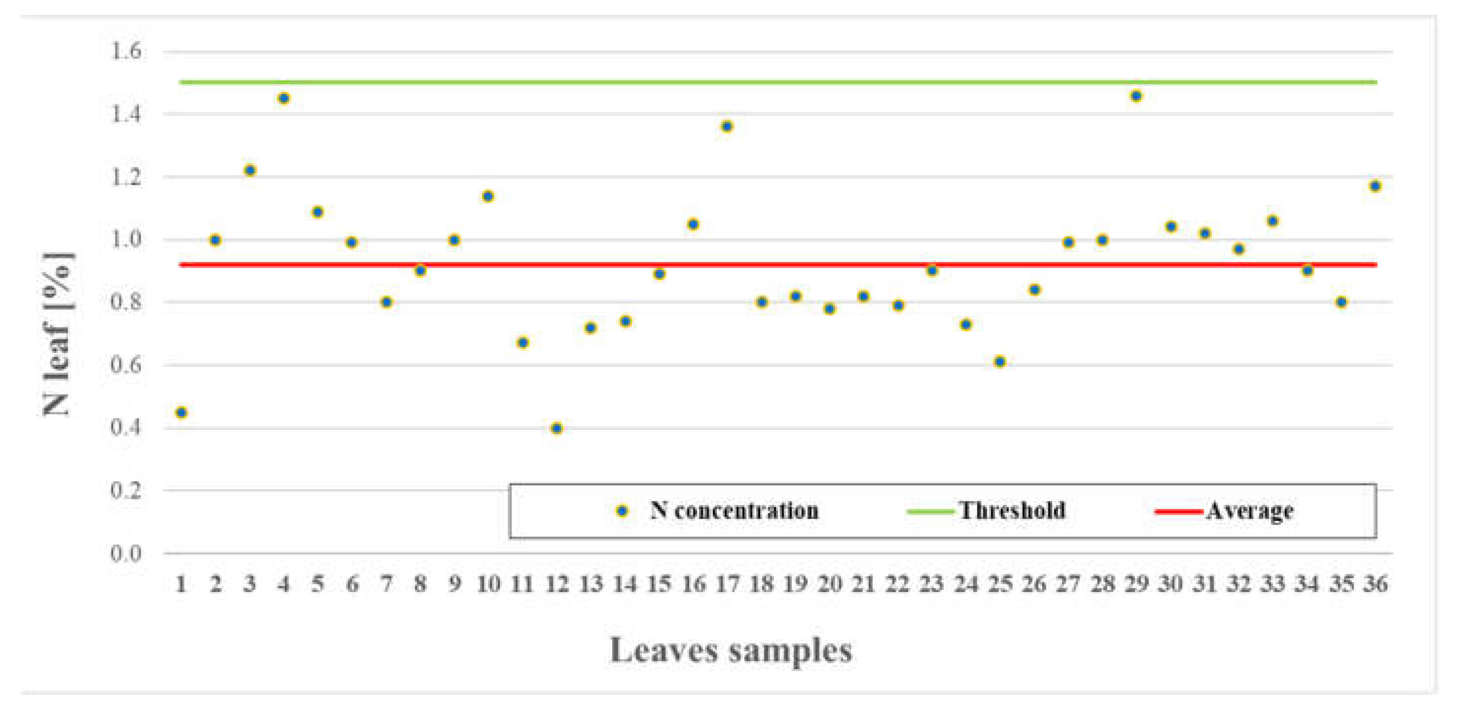
2.3. Soil, Leaf and Drupe Sampling

Field samplings were carried out in order to investigate soil and crop variability. A regular 15 m × 11 m grid was applied in both cases. The sampling points were identified at the intersection (node) of the sampling grid, excluding the most external part of the field. A total number of 36 points was sampled. Soil samples were taken at each intersection points of the grid. Soil sampling was carried out on DOY 168 at a depth from 10 to 30 cm using an Edelman auger. After drying, the soil samples were ground and sieved at <2 mm. Leaf sampling was carried out on DOY 205 [10]. Leaf samples were taken from the four trees situated around the 36 nodes used for soil sampling. Each leaf sample, constituted by 100 leaves, consisted of four sub-samples of 25 healthy, fully expanded, and mature leaves randomly collected from the central portion of current season branches, approximately 1.5 m above the soil surface. After sampling, leaves were dried at 70 °C for 24 h and milled to pass through a 0.25 mm mesh. Drupes sampling was carried out during harvesting. One hundred healthy drupes (25 drupes per tree) were sampled from the four trees used for leaf samples.

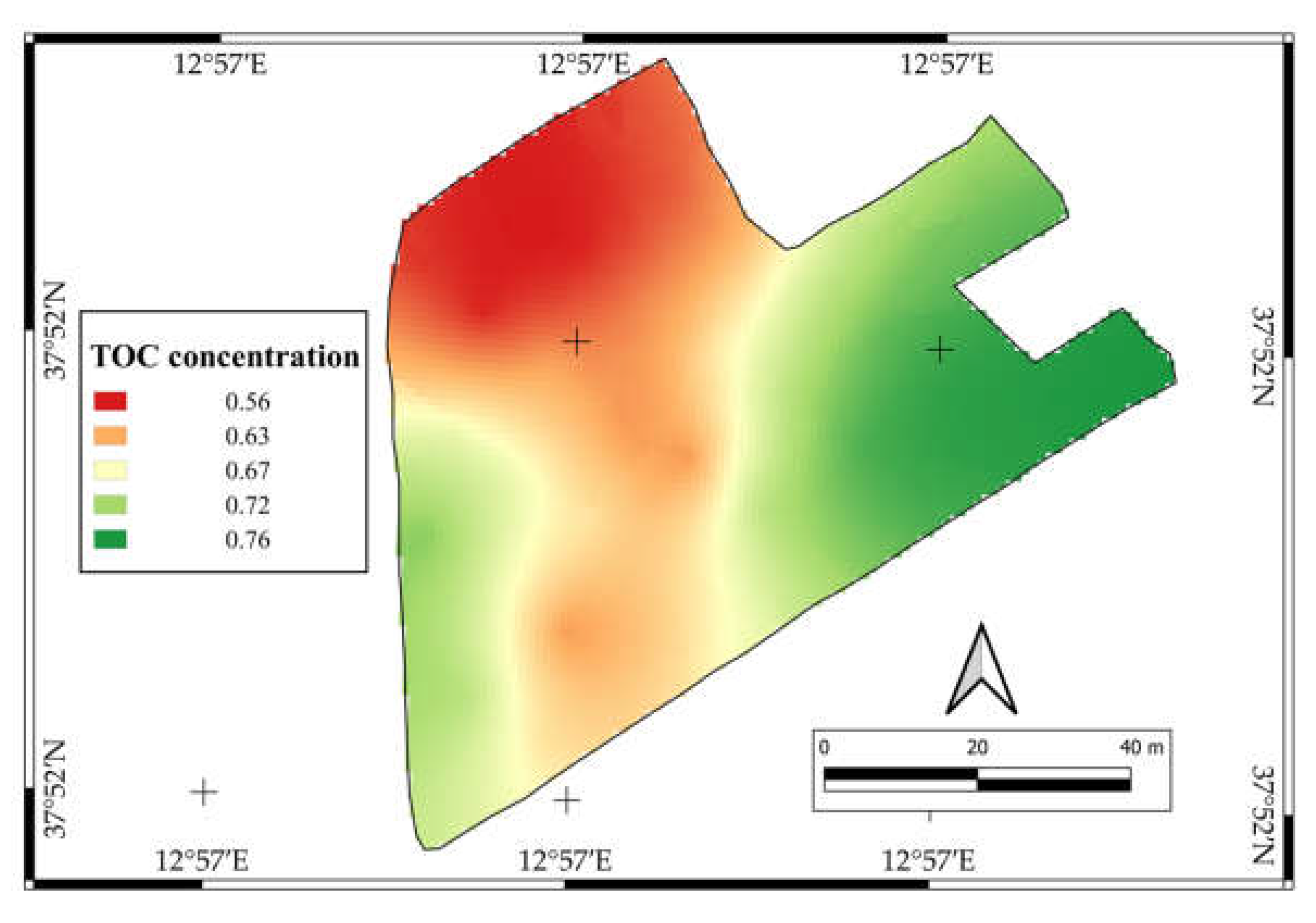
2.4. Laboratory Analysis

Soil samples were analyzed to determine texture, reaction (pH), electrical conductivity (EC), total carbonates (TC), organic carbon (TOC) and total N (TN). Soil texture (sand, 2–0.02 mm; silt, 0.02–0.002 mm; clay, <0.002 mm) was determined by pipette method after shaking soil samples for 2 h with a solution containing sodium hexametaphosphate and sodium carbonate [23]. Soil reaction was measured in distilled water using a soil/solution ratio of 1:2.5 (w/v) and a glass membrane electrode, whereas soil EC was measured in distilled water using a soil/distilled water ratio of 1:5 (w/v). The content of TC was determined by the gas-volumetric method using the Dietrich–Fruehling calcimeter [24]. Soil TOC and TN were determined on pulverized soil samples by the Walkley–Black dichromate oxidation method and the Kjeldahl method, respectively.
Leaf samples were analyzed to determine the total content of the following elements: N, K, Ca, Fe, Mn, Mg, B, Zn, Na, Cu. All elements, except for N, were determined by microwave plasma atomic emission spectrometer (MP-AES 4210, Agilent Technologies, California, CA, USA) after leaf digestion with concentrated nitric acid and hydrogen peroxide. Nitrogen content in leaf and drupes samples was determined by the Kjeldahl method.

2.5. Olive Tree Yield

The production of each tree and that of the whole plot were evaluated quantifying the harvested olives. Olives were harvested when their maturity index was equal to 2.38 determined according to [25]. A team of four operators was employed to harvest the olives. Two of them used the hand-held electric harvester model OLIVION P230 (Pellenc, SI, Italy). The other two operators had the task of laying and wrapping the nets under each plant, before and after harvest. They were also responsible for loading and quantifying the production of each plant. The quantity of the harvested fruits for each plant and the average mass of the drupes were evaluated in the field using two digital balances (Shimadzu ATY324R, Milan, Italy).

2.6. Multispectral Data from UAV

Multispectral data were acquired through an aerial survey using a Phantom4 Multispectral (DJI, Shenzhen, China). The unmanned aerial vehicle (UAV) is equipped with four rotors on a rotating wing. It has a brightness sensor at the top, which allows obtaining pre-calibrated images. It is also capable of image position compensation as the relative positions of the CMOS (Complementary metal–oxide–semiconductor) sensor centers of the six cameras and the phase center of the on-board D-RTK antenna, are stored in the Exif information of each image. The multi-frequency global navigation satellite system (GNSS) positioning system can see and receive signals from the following satellites with their respective frequencies: GPS L1/L2; GLONASS L1/L2; BeiDou B1/B2; Galileo E1/E5.
The multispectral camera has six 1/2.9” CMOS sensors, that is a red-green-blue (RGB) sensor for visible light imaging and five monochrome sensors for multispectral imaging with a final resolution of 2.08 MP pixels. The lens of the multispectral camera has 62.7° FoV (Field of View), 5.74 mm focal length and f/2.2 aperture.

2.7. Flight Scheduling and Images Acquisition

The aerial survey was conducted before sprouting and fertilization on DOY 102 of year 2021. The flight was planned using the official DJI software, which is only available on IOS systems. It was carried out with automatic configuration using the waypoints and RTK mode for correcting geospatial data. The flight was performed at approximately 12:00 noon at a height of 50 m, generating a ground surface distance (GSD) of 2.6 cm. Five GCPs (Ground Control Point) were placed before the flight. The GCPs were georeferenced using the Stonex S7-G instrument above cited. To improve accuracy, the coordinates of the GCPs were acquired by mounting an external dual-frequency antenna (L1/L2; Stonex geodetic antenna) in RTK mode and averaging about 60 coordinate points. Image acquisition was made at an average speed of 10 m s−1 in stop-and-go mode to minimize speed-related distortions. Both front overlap ratio and side overlap ratio were 70% while the gimbal pitch was set at 90° (downwards).

2.8. Data Analysis and Processing

Correlation matrix between soil chemical and physical properties, and plant characteristics was obtained by the software R [26]. For geo-spatial data analysis and processing the open-source software QGIS ver. 3.10 [27] was used. The photogrammetric reconstruction was carried out using Agisoft Photoscan Professional version 1.7.3. A linear model was used, rather than a spherical one, as spatial interpolation method as in [6]. Two interpolation methods, Kriging and triangulated irregular network (TIN) were used to create continuous maps from the discrete point data of soil and crop analysis. In particular, the Kriging method was used to interpolate TOC, TN, leaf N data, while the TIN method was employed to process olive production. The Kriging method, starting from the punctual data, creates a continuous map by interpolating the values based on the distances of the near points. The TIN method considers the point value as an immutable data; it was used to interpolate the production per plant, that was directly measured for each tree, obtaining a continuous map while maintaining the single point information. The maps obtained by using Kriging and TIN methods had the same geometric resolution and extension. Therefore, they are perfectly superimposable layers, with different digital information referable to the different variables investigated; they allowed the realization of the prescription maps for variable rate fertilization through the raster calculator tool in QGIS.

2.9. Nitrogen Balance and Prescription Map Realization

Crop variability, expressed through spectral, biometric, and nutritional parameters, was investigated to describe health status of the olive trees. As a first step, the general nutritional status of the trees was evaluated by determining the nutrient concentration of the leaves. The threshold method of leaves nutrient concentration was used to determine the percentage of the plot area showing deficiency of a given nutrient. The threshold value represents the concentration limit of a nutrient that defines the correct nutritional status of the olive tree. In our study, among the different nutrients, only N had a concentration below the threshold, therefore we focused only on N to draw up the fertilization plan. The threshold value used was N ≥ 1.5% as largely reported in literature [4,19,28].
The N balance (NB) was applied based on the actual needs of each olive plant in the semiarid Mediterranean environment; it can be used for any field/soil type. According to the NB, there are several variables to consider in order to determine the correct amount to be applied [19]. In this experimentation, a simplified version of the NB was proposed, assuming that the olive grove is in vegetative-productive equilibrium. In this case, only the supplementation of the quantities removed and lost during the year to support the following year’s request was needed. Therefore, the fertilization plan was set according to Equation (1), taking into account the amount of nitrogen removed by the production (Nf) and pruning (Nv) and the nitrogen use efficiency (NUE).
F = P     Nf + A Nv   NUE
where F is the amount of fertilizer to be spread per plant (g plant−1), P is the production (kg plant−1), Nf is the nitrogen concentration in the fresh drupes (g kg−1), A is the area attributed to each plant (m2 plant−1), Nv is the amount of nitrogen removed by pruning residues per unit of area (g m−2) and NUE is the nitrogen uptake efficiency (%) set at 45.9% according to [29].
N removal due to olive cultivation is the sum of N removed by drupes harvesting and pruning. N removed by drupes was obtained multiplying the amount of N content of the drupes per amount of the olive harvested. The N removed by drupes was originated from the amount of product and its nitrogen concentration. This concentration was derived from the average amount of N contained in the fresh fruits, and was found to be 2.65 g kg−1 of N. This value was similar to that reported by other studies, such as in [19,28]. The production for plant was determined from the yield map [30].
Since the plot is pruned every two years, during the year of the study it was not possible to obtain data on the amount of pruning residues removed per plant. For this reason, we used the average canopy area of the plants as a starting point for constructing the vigour ratios between neighboring plants. Images acquired during the flight with UAV was used to produce an NDVI map describing the vigor of each of plant [31]. This Vegetation Index (VI) is the main VI used in the bibliography to determine the principal vigor characteristic [32]. It was calculated [33] using the Equation (2).
NDVI = ρ NIR ρ Red ρ NIR + ρ RED
Starting from the NDVI map, the GIS processing was used to extract the canopy area of each plant [31] using several GEOBIA (geographic object-based image analysis) steps. The first step was image segmentation to differentiate the canopy from the background. It was performed using the K-means algorithm executed in a Saga tool of raster image analysis. Subsequently, through a process of rasterization and a vectorialization algorithm, it was possible to extract the different canopy areas and relative information. The real area available for each plant according to its vigor was calculated by following the vigor gradient between plants using the Voronoi polygon [27] function. The amount of N removed by each plant with pruning residues was calculated by multiplying the new area attributed to each plant per the amount of N per square meter. This value was derived from the literature considering that 36 kg of N per hectare per year are removed by olive plants [19], that means 3.6 g N m−2 year−1. Finally, the amount of fertilizer to be distributed per plant was quantified according to Equation (1) by adjusting it on the basis of the NUE [29].
The prescription map of the entire studied plot was created by considering the area attributed to each plant and the amount of N to be distributed per plant. The prescription map had a resolution of 1 m2 (1 pixel) containing, as digital number (DN), the amount of N to be distributed per square meter. The prescription map allowed for the precision fertilization to be carried out by normal pneumatic spreaders and also with centrifugal spreaders with the appropriate calibrations [34].

3. Results

The main characteristics of the soil of the studied area are reported in Table 1. According to the ISSS (International Society of Soil Science) classification system of soil particles, soil texture was sandy clay loam [35]. Soil reaction was neutral whereas both total carbonates and electrical conductivity (EC) showed low values. Total organic carbon and nitrogen concentration were also low.
Total N ranged from 0.10% to 0.25% and was positively related with TOC (r = 0.52 **). The map describing soil TOC spatial variability was provided through the interpolation with geostatic methods (Figure 2).
Sand, electrical conductivity, organic matter and total N values were positively correlated with some crop variables such as TCSA, yield, NDVI and canopy area (Table 2) thus suggesting the importance of soil fertility and nitrogen for olive orchard growth. Strong correlations were obtained, in particular, between NDVI and canopy area (r = 0.90 ***). The best correlation of TCSA was obtained with the canopy area (r = 0.78 ***). All the vegetative parameters showed an important correlation with yield, especially NDVI (r = 0.70 ***) and canopy area (r = 0.76 ***).
With regard to the crop nutritional status, of the nine elements determined by the leaf samples to assess nutrient deficiencies (Table 3), only nitrogen had a concentration below the threshold [4,17,36]. Indeed, the total N concentration of plant leaves ranged from 0.40% to 1.46%, being on average 0.92% (Figure 3).
The canopy area was extracted from the NDVI map (Figure 4) and enable to design the vigor ratio among the neighbouring plants before obtaining the prescription map, as explained in the materials and methods.
Total olive yield during the study year was 2.8 t, corresponding to 4.8 t ha−1 (12.8 kg plant−1). Olive production and canopy area based on NDVI were overlapped in Figure 5, also showing a certain variability in olive yield.
The amount of N to be applied ranged from 7.5 to 18.5 g per square meter, corresponding on average to 255 g per plant. Figure 6 represents the prescription map of the amount of N to be applied. The plants were grouped into four different classes, according to the corresponding quartile.

4. Discussion

Geostatistical analysis of the maps enabled us to trace the spatial variability of the main soil variables such as texture, pH, electrical conductivity and TOC and TN. The production of olive trees was influenced by soil fertility, and particularly the amount of TN and TOC as found in similar studies (e.g., [1]). In the whole experimental area, the concentration of TOC, as well as total N, was low probably due to concomitant factors: (i) excessive mineralization of organic matter; and (ii) the lack of organic matter supply [37]. The low amount of foliar nitrogen, thus, may be explained by the low concentration of soil nitrogen. Indeed, the foliar N concentration values were all lower than the threshold, although in line with previous studies [3,10].
However, soil parameters showed a good correlation with plant nutrition and vegetative status. Olive production was influenced by soil fertility, particularly TN and TOC. TOC was correlated with vegetative activity (NDVI and canopy area) and production while TN was correlated only with production. Probably, TN did not correlate closely with vegetative parameters because these are influenced by many variables such as pruning, agronomic management, etc. and not only by nitrogen availability, which fluctuates over the years.
The experiment showed that the entire plot area had nitrogen deficiency, as all samples had N concentration below the optimal threshold of 1.5%. No values below the threshold were observed for any of the other elements based on the work of Marãn and Fernãndez-Escobar [4]. For this reason it was not possible to exclude zones of the plot from N fertilization [10,18,38].
Canopy area and NDVI reflect the real vegetative status of the plants at the moment in which they are determined. Since they are significantly correlated with TCSA, this finding suggests the good ability of the remote sensing platform (UAV) to detect and investigate the variability of vigour in the olive grove [2,18], thus minimising field sampling [39,40]. Furthermore, the vegetative characteristics had a significant and robust correlation with production. It confirms that production was strongly influenced by the spectral and biometric characteristics of the crop and their correct management can improve the quality and the quantity of the products [8]. Therefore, by having a broad knowledge of the field conditions, it is also possible to trace the production, as other studies have proved [41].
The amount of fertilizer actually saved per hectare compared to normal distributions was then evaluated. A careful survey of the surrounding area showed that the dose of nitrogen commonly used is about 150 kg ha−1, which corresponds to 88 kg in our plot. However, based on Equation (1), the actual amount of nitrogen to be applied is 60 kg. This amount corresponds to 20 kg of nitrogen immobilized and used for vegetative activity and 8 kg of N was contributed by production. Thus, the quantity to be actually distributed was 102 kg ha−1. Therefore, a fertilizer saving of 47 kg ha−1 was obtained, i.e., 31% less than the standard and homogeneous dose as obtained in previous studies [14,38].

5. Conclusions

A methodology was proposed in this study to create a prescription map for fertilizers applied in an olive orchard, taking into account the actual agronomic and soil conditions of the agro-ecosystem. Productivity, biometric, nutritional, and spectral data of the olive trees provided important information for deriving the correct crop nitrogen requirements for each individual plant. In particular, for the application of precision nitrogen fertilization, productivity, the amount of biomass produced, and the relative nitrogen concentration were needed. By integrating the different information, an even more accurate estimate of nitrogen requirements was obtained, taking into account the crop and the current agronomic conditions. A 31% fertilizer savings was obtained, with economic, agronomic, and environmental benefits. In particular, from an environmental point of view, the reduction of distributed nitrogen limits the process of loss by leaching with consequent pollution of surface and groundwater. Overall, this method determined a reduction in fertilizers distribution, lowering total costs, and reaching greater sustainability.

Author Contributions

Conceptualization, P.C. and V.A.L.; methodology, P.C. and M.V.; validation, P.C., V.A.L. and M.V.; formal analysis, E.R. and P.C.; investigation, E.R.; resources, P.C. and V.A.L.; data curation, E.R. and P.C.; writing—original draft preparation, E.R.; writing—review and editing, V.A.L. and M.V.; visualization, E.R., V.A.L. and M.V.; supervision, P.C. and M.V.; project administration, P.C. All authors have read and agreed to the published version of the manuscript.

Funding

This research received no external funding.

Data Availability Statement

Not applicable.

Conflicts of Interest

The authors declare no conflict of interest.

References

  1. Fountas, S.; Aggelopoulou, K.; Gemtos, T.A. Precision Agriculture: Crop Management for Improved Productivity and Reduced Environmental Impact or Improved Sustainability. In Supply Chain Management for Sustainable Food Networks; John Wiley & Sons, Inc.: Hoboken, NJ, USA, 2015; pp. 41–65. [Google Scholar]
  2. Roma, E.; Catania, P. Precision Oliviculture: Research Topics, Challenges, and Opportunities—A Review. Remote Sens. 2022, 14, 1668. [Google Scholar] [CrossRef]
  3. Fernández-Escobar, R.; Marín, L. Nitrogen Fertilization in Olive Orchards. In Proceedings of the III International Symposium on Olive Growing, Crete, Greece, 22–26 September 1997; pp. 333–336. [Google Scholar]
  4. Marãn, L.; Fernãndez-Escobar, R. Optimization of Nitrogen Fertilization in Olive Orchards. In Proceedings of the III International Symposium on Mineral Nutrition of Deciduous Fruit Trees, Zaragoza, Spain, 27–31 May 1996; pp. 411–414. [Google Scholar]
  5. Agam, N.; Segal, E.; Peeters, A.; Levi, A.; Dag, A.; Yermiyahu, U.; Ben-Gal, A. Spatial Distribution of Water Status in Irrigated Olive Orchards by Thermal Imaging. Precis. Agric. 2014, 15, 346–359. [Google Scholar] [CrossRef]
  6. Álamo, S.; Ramos, M.; Feito, F.; Cañas, A. Precision Techniques for Improving the Management of the Olive Groves of Southern Spain. Span. J. Agric. Res. 2012, 10, 583–595. [Google Scholar] [CrossRef] [Green Version]
  7. Fernández-Escobar, R. Use and Abuse of Nitrogen in Olive Fertilization. Acta Hortic. 2011, 888, 249–257. [Google Scholar] [CrossRef]
  8. Fernandez-Escobar, R.; Ortiz-Urquiza, A.; Prado, M.; Rapoport, H.F. Nitrogen Status Influence on Olive Tree Flower Quality and Ovule Longevity. Environ. Exp. Bot. 2008, 64, 113–119. [Google Scholar] [CrossRef]
  9. Zipori, I.; Erel, R.; Yermiyahu, U.; Ben-Gal, A.; Dag, A. Sustainable Management of Olive Orchard Nutrition: A Review. Agriculture 2020, 10, 11. [Google Scholar] [CrossRef] [Green Version]
  10. López-Granados, F.; Jurado-Expósito, M.; Alamo, S.; Garcıa-Torres, L. Leaf Nutrient Spatial Variability and Site-Specific Fertilization Maps within Olive (Olea europaea L.) Orchards. Eur. J. Agron. 2004, 21, 209–222. [Google Scholar] [CrossRef]
  11. Rubio-Delgado, J.; Pérez, C.J.; Vega-Rodríguez, M.A. Predicting Leaf Nitrogen Content in Olive Trees Using Hyperspectral Data for Precision Agriculture. Precis. Agric. 2021, 22, 1–21. [Google Scholar] [CrossRef]
  12. Dag, A.; Ben-David, E.; Kerem, Z.; Ben-Gal, A.; Erel, R.; Basheer, L.; Yermiyahu, U. Olive Oil Composition as a Function of Nitrogen, Phosphorus and Potassium Plant Nutrition. J. Sci. Food Agric. 2009, 89, 1871–1878. [Google Scholar] [CrossRef]
  13. Tognetti, R.; Morales-Sillero, A.; d’Andria, R.; Fernandez, J.; Lavini, A.; Sebastiani, L.; Troncoso, A. Deficit Irrigation and Fertigation Practices in Olive Growing: Convergences and Divergences in Two Case Studies. Plant Biosyst. 2008, 142, 138–148. [Google Scholar] [CrossRef]
  14. Van Evert, F.K.; Gaitán-Cremaschi, D.; Fountas, S.; Kempenaar, C. Can Precision Agriculture Increase the Profitability and Sustainability of the Production of Potatoes and Olives? Sustainability 2017, 9, 1863. [Google Scholar] [CrossRef] [Green Version]
  15. Agüera-Vega, J.; Blanco, G.; Castillo, F.; Castro-Garcia, S.; Gil-Ribes, J.; Perez-Ruiz, M. Determination of Field Capacity and Yield Mapping in Olive Harvesting Using Remote Data Acquisition. In Precision Agriculture’13; Wageningen Academic Publishers: Wageningen, The Netherlands, 2013; pp. 691–696. [Google Scholar]
  16. Castillo-Ruiz, F.J.; Pérez-Ruiz, M.; Blanco-Roldán, G.L.; Gil-Ribes, J.A.; Agüera, J. Development of a Telemetry and Yield-Mapping System of Olive Harvester. Sensors 2015, 15, 4001–4018. [Google Scholar] [CrossRef] [PubMed] [Green Version]
  17. Akdemir, B.; Saglam, C.; Belliturk, K.; Makaraci, A.; Urusan, A.; Atar, E. Effect of Spatial Variability on Fertiliser Requirement of Olive Orchard Cultivated for Oil Production. J. Environ. Prot. Ecol. 2018, 19, 319–329. [Google Scholar]
  18. Noori, O.; Panda, S.S. Site-Specific Management of Common Olive: Remote Sensing, Geospatial, and Advanced Image Processing Applications. Comput. Electron. Agric. 2016, 127, 680–689. [Google Scholar] [CrossRef]
  19. Fernández-Escobar, R.; García-Novelo, J.; Molina-Soria, C.; Parra, M. An Approach to Nitrogen Balance in Olive Orchards. Sci. Hortic. 2012, 135, 219–226. [Google Scholar] [CrossRef]
  20. Kottek, M.; Grieser, J.; Beck, C.; Rudolf, B.; Rubel, F. World Map of the Köppen-Geiger Climate Classification Updated. Meteorol. Z. 2006, 15, 259–263. [Google Scholar] [CrossRef] [PubMed]
  21. Catania, P.; Comparetti, A.; Febo, P.; Morello, G.; Orlando, S.; Roma, E.; Vallone, M. Positioning Accuracy Comparison of GNSS Receivers Used for Mapping and Guidance of Agricultural Machines. Agronomy 2020, 10, 924. [Google Scholar] [CrossRef]
  22. Catania, P.; Orlando, S.; Roma, E.; Vallone, M. Vineyard Design Supported by GPS Application. Acta Hortic. 2021, 1314, 227–234. [Google Scholar] [CrossRef]
  23. Gee, G.W.; Or, D. 2.4 Particle-size Analysis. In Methods of Soil Analysis: Part 4 Physical Methods; John Wiley & Sons, Inc.: Hoboken, NJ, USA, 2002; Volume 5, pp. 255–293. [Google Scholar]
  24. Williams, D. A Rapid Manometric Method for the Determination of Carbonate in Soils. Soil Sci. Soc. Am. J. 1949, 13, 127–129. [Google Scholar] [CrossRef] [Green Version]
  25. Furferi, R.; Governi, L.; Volpe, Y. ANN-Based Method for Olive Ripening Index Automatic Prediction. J. Food Eng. 2010, 101, 318–328. [Google Scholar] [CrossRef] [Green Version]
  26. R Core Team. R: A Language and Environment for Statistical Computing; R Foundation for Statistical Computing: Vienna, Austria, 2021; Available online: https://www.R-project.org/ (accessed on 12 April 2022).
  27. QGIS Geographic Information System. QGIS Association. 2022. Available online: QGIS.org (accessed on 12 April 2022).
  28. Fernández-Escobar, R.; Sánchez-Zamora, M.A.; Garcia-Novelo, J.M.; Molina-Soria, C. Nutrient Removal from Olive Trees by Fruit Yield and Pruning. HortScience 2015, 50, 474–478. [Google Scholar] [CrossRef]
  29. Fernández-Escobar, R.; Antonaya-Baena, M.; Sánchez-Zamora, M.; Molina-Soria, C. The Amount of Nitrogen Applied and Nutritional Status of Olive Plants Affect Nitrogen Uptake Efficiency. Sci. Hortic. 2014, 167, 1–4. [Google Scholar] [CrossRef]
  30. Blackmore, S. The Role of Yield Maps in Precision Farming. Ph.D. Thesis, Cranfield University, Bedford, UK, 2003. [Google Scholar]
  31. Caruso, G.; Zarco-Tejada, P.J.; González-Dugo, V.; Moriondo, M.; Tozzini, L.; Palai, G.; Rallo, G.; Hornero, A.; Primicerio, J.; Gucci, R. High-Resolution Imagery Acquired from an Unmanned Platform to Estimate Biophysical and Geometrical Parameters of Olive Trees under Different Irrigation Regimes. PLoS ONE 2019, 14, e0210804. [Google Scholar] [CrossRef] [PubMed] [Green Version]
  32. Xue, J.; Su, B. Significant Remote Sensing Vegetation Indices: A Review of Developments and Applications. J. Sens. 2017, 2017, 1353691. [Google Scholar] [CrossRef] [Green Version]
  33. Rouse, J.W.; Haas, R.H.; Schell, J.A.; Deering, D.W.; Harlan, J.C. Monitoring the Vernal Advancement and Retrogradation (Green Wave Effect) of Natural Vegetation; NASA/GSFC Type III Final Report, Greenbelt, Md; NTRS: Chicago, IL, USA, 1974; Volume 371. [Google Scholar]
  34. Cointault, F.; Sarrazin, P.; Paindavoine, M. Measurement of the Motion of Fertilizer Particles Leaving a Centrifugal Spreader Using a Fast Imaging System. Precis. Agric. 2003, 4, 279–295. [Google Scholar] [CrossRef]
  35. Hillel, D. Fundamentals of Soil Physics; Academic Press: Cambridge, MA, USA, 2013; ISBN 0-08-091870-0. [Google Scholar]
  36. Barranco Navero, D.; Fernandez Escobar, R.; Rallo Romero, L. El Cultivo del Olivo, 7th ed.; Mundi-Prensa Libros: Barcelona, Spain, 2017; ISBN 84-8476-714-0. [Google Scholar]
  37. Laudicina, V.A.; Hurtado, M.D.; Badalucco, L.; Delgado, A.; Palazzolo, E.; Panno, M. Soil Chemical and Biochemical Properties of a Salt-Marsh Alluvial Spanish Area after Long-Term Reclamation. Biol. Fertil. Soils 2009, 45, 691–700. [Google Scholar] [CrossRef]
  38. Aggelopoulou, K.; Pateras, D.; Fountas, S.; Gemtos, T.; Nanos, G. Soil Spatial Variability and Site-Specific Fertilization Maps in an Apple Orchard. Precis. Agric. 2011, 12, 118–129. [Google Scholar] [CrossRef]
  39. Fulton, J.P.; Port, K. Precision Agriculture Data Management. In Precision Agriculture Basics; John Wiley & Sons, Inc.: Hoboken, NJ, USA, 2018; pp. 169–187. [Google Scholar]
  40. Shafi, U.; Mumtaz, R.; García-Nieto, J.; Hassan, S.A.; Zaidi, S.A.R.; Iqbal, N. Precision Agriculture Techniques and Practices: From Considerations to Applications. Sensors 2019, 19, 3796. [Google Scholar] [CrossRef] [Green Version]
  41. Stateras, D.; Kalivas, D. Assessment of Olive Tree Canopy Characteristics and Yield Forecast Model Using High Resolution UAV Imagery. Agriculture 2020, 10, 385. [Google Scholar] [CrossRef]
Figure 1. (a) Experimental site location on a scale of 1:1,200,000; (b) study area.
Agronomy 13 00324 g001
Figure 2. TOC (%) map of the study area.
Agronomy 13 00324 g002
Figure 3. Nitrogen concentration determined on 36 leaf samples uniformly collected from olive plants. The red line represents the average of the whole samples, while the green line represents the threshold.
Agronomy 13 00324 g003
Figure 4. Canopy area and NDVI value for each plant in a portion of the plot.
Agronomy 13 00324 g004
Figure 5. (a) Overlay between the production map (red-green scale) and the individual tree canopy with coloration according to NDVI value; and (b) particular of the image.
Agronomy 13 00324 g005
Figure 6. Prescription map of nitrogen fertilization according to the different quantity of nitrogen per square meter.
Agronomy 13 00324 g006
Table 1. Characteristics of the soil of the studied area.
ParameterMeanSDCV (%)
Clay (%)303.3011
Silt (%)131.9215
Sand (%)574.017
Total organic carbon (%)0.670.1014
Total nitrogen (%)0.150.0320
Total carbonates (%)5.093.2364
pH7.240.182
Electrical conductivity (dS m−1)0.160.0317
Table 2. Correlation among the main soil, vegetative and production parameters. Electrical conductivity (EC, dS m−1); Total carbonates (TC, %); Sandy (%); Total Organic Carbon (TOC, %); Soil Nitrogen (Ns, %); Leaf Nitrogen (Nf, %); Leaf Potassium (K, %); Leaf Calcium (Ca, %); Leaf Iron (Fe, %), Leaf Magnesium (Mg, %); Leaf Manganese (Mn, ppm); Leaf Zinc (Zn, ppm); Leaf Copper (Cu, ppm); Yield (kg); TCSA (m2); NDVI; Canopy area (m2). * p value < 0.05; ** p value < 0.01; *** p value < 0.001.
ECTCSandyTOCNsNfKCaFeMgMnZnTCSAYieldNDVI
Ns0.130.300.020.52 ***
K−0.130.43 **0.10−0.240.35 *0.30
Ca−0.030.42 **0.03−0.120.38 *0.250.91 ***
Mg−0.130.270.00−0.230.100.38 *0.80 ***0.82 ***0.28
Mn−0.040.63 ***0.00−0.020.43 **0.270.92 ***0.85 ***−0.100.70 ***
Zn−0.040.000.02−0.320.000.36 *0.62 ***0.68 ***0.41 *0.82 ***0.40 *
Cu−0.08−0.16−0.07−0.370.050.000.310.47 **0.52 ***0.48 **0.060.74 ***
TCSA0.35 *−0.020.200.240.12−0.28−0.37−0.170.10−0.45−0.29−0.35
Yield0.200.120.49 **0.34 *0.42 ***−0.04−0.110.03−0.04−0.24−0.07−0.230.53 ***
NDVI0.30−0.100.34 **0.42 **0.120.01−0.39−0.210.20−0.38−0.30−0.250.73 ***0.69 ***
Canopy area0.21−0.030.37 **0.33 *0.13−0.10−0.33−0.130.14−0.36−0.27−0.260.78 ***0.76 ***0.90 ***
Table 3. Leaf elements concentration and corresponding threshold [4,17,36].
ElementMean Value ± st.dev.Threshold
N [%]0.92 ± 0.23≥1.5
K [%]1.00 ± 0.57≥0.8
Ca [%]0.66 ± 0.24≥0.5
Fe [%]0.45 ± 0.28≥0.1
Mg [%]0.52 ± 0.38≥0.1
Mn [ppm]0.12 ± 0.02≥0.06
Zn [ppm]0.11 ± 0.02≥0.06
Cu [ppm]0.09± 0.02≥0.06
Disclaimer/Publisher’s Note: The statements, opinions and data contained in all publications are solely those of the individual author(s) and contributor(s) and not of MDPI and/or the editor(s). MDPI and/or the editor(s) disclaim responsibility for any injury to people or property resulting from any ideas, methods, instructions or products referred to in the content.

