Validating the Contribution of Nature-Based Farming Solutions (NBFS) to Agrobiodiversity Values through a Multi-Scale Landscape Approach

Abstract

Nature-Based Farming Solutions (NBFS) are envisaged practices that still strongly demand further context-specific scientific validation for their viable deployment at the local scale. In this context, our study deals with the test of a multi-scale system of landscape ecology indicators, interpreted as surrogates for the accounting of the contributions of NBFS to agrobiodiversity values and to the consequent environmental stability and resilience capacities of agroecosystems, recognized as pivotal for facing the ongoing climate change challenges. We here present the preliminary results obtained in a first pilot case study (Po Plain context). Landscape ecology analyses were undertaken at extra-local, local, and farm scales (with different levels of analytical detail), comparing the pilot farm to the surrounding conventionally managed context. A set of structural and functional indicators were tested, allowing a preliminary screening of the most suitable ones (good sensitivity to treatment changes, informative potential). Results suggested a multi-faceted positive contribution given by NBFS implementation and were the basis for orienting further NBFS implementation strategies based on vulnerability and resilience properties analysis. Further investigations are envisaged on wider datasets coming from other pilot case studies belonging to similar pedo-climatic conditions, in order to improve the informative potential of the here presented methodology.

1. Introduction

Nature-Based Farming Solutions (NBFS) (here intended as landscape feature creation and maintenance across the rural landscape, agroforestry practices, and crop diversification) are oriented towards the reintegration, within the agricultural systems, of their undermined ecosystem functions [1,2,3,4,5,6,7,8]. Thus, they are aimed at enhancing the environmental stability, resistance, and resilience capacity [9] of agroecosystems and their consequent climate change adaptation and mitigation suitability [10,11,12,13,14,15,16,17,18,19,20,21]. The latest European and worldwide agri-environmental policies and sustainable development strategies are recognizing such integrated approaches as pivotal [22,23,24,25,26,27,28,29,30].

Despite these premises, consistent and successful integration of NBFS among real farming systems has been delayed despite its claimed urgency [10,31,32,33]. European and national public subsidies are supporting such approaches through diversified policy tools [5,13], which are mainly derived from practice-based evaluation approaches. Result-oriented approaches would overcome the limits of linking subsidies to pre-established specific practices. Indeed, they would allow the support of a farm management model as a whole on the basis of its recognised positive influence on significant agri-environmental indicators [13,32,34], accounting for an influence on ecological functions. Nonetheless, result-based approaches still need to be fully developed (first of all, by overcoming cost-efficiency performance limits), calibrated, and validated among specific pedo-climatic contexts in order to be successfully integrated into the different levels of policy and accreditation tools [11,32,35,36,37,38,39,40,41]. Hybrid assessment schemes (both practice- and result-based) are often the most viable solution [35]. Different experiences already exist with integrated, result-based, and hybrid agrobiodiversity indicator monitoring systems [40,42,43,44,45,46,47,48,49]. Multi-scale analytical approaches are envisaged for such kinds of assessments, as field-scale biodiversity is intrinsically influenced by factors working on different spatial scales [15,50,51]. Nonetheless, general concepts, theories, and models linking biodiversity to landscape scale parameters only allow us to use them as a surrogate of agrobiodiversity values [52], while their use as a correlate to biodiversity values still needs context specific validation [49,52]. Given this, landscape ecology tools [53,54,55,56,57,58,59] validated for specific contexts offer a viable double contribution, both accounting for structural (in link with management options) and functional traits (in link with results derived from management options).

In continuity with this framework, our project deals with a context-specific test, calibration, and validation of a multi-scale landscape ecology indicators system through the study of organic farming systems adopting agroecological practices that can be ascribed to the NBFS approach [5,60]. The final aim is the selection of a viable set of indicators effective in synthesizing the contributions of NBFS to overall farm agrobiodiversity values and, in parallel, the orientation of further NBFS implementation strategies [61,62]. The contexts under study are located among different districts of the Po Plain system (North of Italy), sharing similar (but not identical) climatic conditions, and representing different pedological case histories of this alluvial macro-context.

In this paper, we present preliminary results from a first pilot case study compared to its surrounding conventionally managed agricultural situation. These results, which already highlighted positive trends on the studied pilot farm, are interpreted here as a surrogate representation of agrobiodiversity values from a hybrid practice and result-based perspective. The in-plan comparison of the here-presented results with floristic-vegetational indicators [63,64,65,66,67] will allow for their use as a correlate to biodiversity values [52]. This will further extend their informative potential on the ecological patterns and trends resulting from farmland agroecological management through the NBFS [6,42,43,68,69,70,71,72,73,74], while also orienting its strategic redesign through time [3,4,61,62,75,76,77,78,79,80].

2. Materials and Methods

2.1. The Adopted Landscape Ecology Analytical Approach

Landscape ecological structural and functional traits were studied following a multi-scale approach (extra-local scale; local scale (La); and farm scale (Fa)) (Figure 1), making reference to the landscape ecology [53,54,55,56,57,58,81] and landscape bionomics methodologies [78,82,83]. The set of indicators to be analyzed was set up, including physiognomic-structural, functional, and dynamic information levels on the landscape system. Appendix A;

Table A1. Set of indicators under study.

	Indicators	Equation	References
PATCHES METRICS	Medium patches size (MPS)	$MPS=\frac{{{\displaystyle \sum }}_{i=1}^n{A}_i/N_i}{LU}$ Ai = total area of each land use categories patches Ni = no. of patches for each land use categories LU = no. of land use categories	[59]
	Matrix (MTX)	$MTX=\frac{{{\displaystyle \sum }}_{i=1}^n{A}_i\times 100}{A_{tot}}$ Ai = total area of each land use categories patches Atot = total area	[59]
SHAPE INDICES	Mean Perimeter area ratio (MPAR)	$MPAR=\frac{{{\displaystyle \sum }}_{i=1}^{n}PA{R}_i}{NP}$ $PA{R}_i=\frac{P_i}{A_i}$ Pi = Perimeter of each land use category patches NP = total no. of patches	[69]
	Shape index (SI)	$SI=\frac{ P_i}{2\times \sqrt{\pi \times A_i}}$	[69]
	Mean Shape Index (MSI)	$MSI=\frac{{{\displaystyle \sum }}_{i=1}^{n}SI}{NP}$	[69]
	Area weighted mean shape index (AWSI)	$AWSI=\frac{{{\displaystyle \sum }}_{i=1}^{n}SI\times A_i}{{{\displaystyle \sum }}_{i=1}^n{A}_i}$	[69]
	Patch fractal dimension (PFD)	$PFD=\frac{2\times \ln P_i}{\ln A_i}$	[59,69]
	Mean patch fractal dimension (MPFD)	$MPFD=\frac{{{\displaystyle \sum }}_{i=1}^{n}PF{D}_i}{NP}$	[69]
	Area weighted mean patch fractal dimension (AWPFD)	$AWPFD=\frac{{{\displaystyle \sum }}_{i=1}^{n}PF{D}_i\times A_i}{{{\displaystyle \sum }}_{i=1}^n{A}_i}$	[69]
COMPOSITION INDICES	Diversity_1a/tot (DIV1a)	$DI{V}_{1a}=-{\displaystyle \sum }_{i=1}^n\frac{A_i}{A_{tot}}\times \ln \frac{A_i}{A_{tot}}$	[59]
	Diversity_1b/landscape element (DIV1b)	$DI{V}_{1b}=-{\displaystyle \sum }_{i=1}^n\frac{A_i}{A_y}\times \ln \frac{A_i}{A_y}$ Ay = total area of each landscape system (natural, agricultural, and anthropic)	[59]
	Diversity_2 (DIV2)	$DI{V}_2=\frac{-{{\displaystyle \sum }}_{i=1}^n\frac{A_i}{A_{tot}}\times \ln \frac{A_i}{A_{tot}}}{\ln S}$ lnS = max(DIV) S = no. of land use categories	[59,142]
	Dominance_1 (DOM1)	$DO{M}_1=\ln S+{\displaystyle \sum }_{i=1}^n\frac{A_i}{A_{tot}}\times \ln \frac{A_i}{A_{tot}}$	[82,84]
	Dominance_2 (DOM2)	$DO{M}_2=\ln S+\frac{{{\displaystyle \sum }}_{i=1}^n\frac{A_i}{A_{tot}}\times \ln \frac{A_i}{A_{tot}}}{\ln S}$	[59]
	Landscape Structural Diversity_1 (LSD1)	$LS{D}_1=DI{V}_1\times \left(3+DO{M}_1\right)$	[82,84]
	Landscape Structural Diversity_2 (LSD2)	$LS{D}_2=DI{V}_2\times \left(3+DO{M}_2\right)$	[82,84]
CONNECTIVITY INDICES	Connectivity (CON)	$CON=\frac{L}{\left[3\times \left(N-2\right)\right]}$ L = no. of links N = no. of nodes	[95]
	Weighted connectivity (WCON)	$WCON=\frac{{{\displaystyle \sum }}_{i=1}^5{L}_i\times W_i}{[3\times (N-2)]}$ Li = no. of links for each Ecological Quality Class (EQCi = [1–5]) Wi = EQCi weight: $W_i=\frac{EQ{C}_i}{EQ{C}_{max}}$	[95] modified by authors
	Circuitry (CIR)	$CIR=\frac{\left(L-N+1\right)}{\left[2\times \left(N-5\right)\right]}$	[95]
	Weighted circuitry (WCIR)	$WCIR=\frac{[({{\displaystyle \sum }}_{i=1}^5{L}_i\times W_i)-N+1)]}{\left[2\times \left(N-5\right)\right]}$ Li = no. of links for each Ecological Quality Class (EQCi = [1–5]) Wi = EQCi weight (as above)	[95] modified by authors
FUNCTIONALITY INDICES	Biological Territorial Capacity (BTC)	$BTC={\displaystyle \sum }_{i=1}^{n}BT{C}_i\times A_i$ BTCi = BTC value attributed to each land use category (tabulated values; see references)	[73,94]

lists: (i) the set of indicators under study; (ii) the related formulas; and (iii) the main references for each indicator under study (Appendix A; Table A1). Potentially redundant variants of the same indicator categories were included. The aim was to: (i) assess their sensitiveness to the compared management options among the specific studied context; and (ii) consequently, identify a preliminary sub-set of independent (low correlation coefficients values) and highly sensitive indicators, that were viable for the project’s purposes.

Extra-local and local scale boundaries were identified according to the landscape unit and ecotope concepts developed by Ingegnoli [78,82,84]. The ratio of local scale to extra-local scale surface resulted in about 1% (3.44 km² and 312.05 km², respectively). Farm scale boundaries were set coincident to farm’s patches boundaries (0.12 km²), even if discontinuous, in order to only take into account in-farm management options effects.

Figure 1. (a) Pilot farm location among the regional, extra-local, and local contexts, along the Ticino River basin; (b) land cover at local scale (LCP 2010, Piedmont region [85]), showing the current landscape patches and linear corridors (as used for landscape metrics computing), compared to historical traits.

Figure 1. (a) Pilot farm location among the regional, extra-local, and local contexts, along the Ticino River basin; (b) land cover at local scale (LCP 2010, Piedmont region [85]), showing the current landscape patches and linear corridors (as used for landscape metrics computing), compared to historical traits.

Spatial-qualitative featuring of the extra-local and local scale analytical units was based on the following GIS information [85,86,87]: geomorphology, pedology, hydrology, phyto-climate, regional land cover, historical land use, vegetation, protected areas, regional ecological network, and other in-force land-planning tools. At an extra-local scale, this preliminary context informed an exploratory vulnerability and resilience (VR) analysis [88,89,90,91,92]. For local scales, GIS data were validated through coarse field surveys.

At La and Fa scales, current landscape mosaic structural elements (matrix, patches, and corridors) were mapped as vectors on QGIS software (the minimum patch size was set to 70 m²) and quantified [by number, relative surfaces, and perimeters cumulated for each land use significant category, clustered in 3 landscape sub-systems: natural (NAT), agricultural (AGR), and anthropic (ANT) (Figure 1)]. Preliminary framing analyses were carried out on landscape physiological apparatuses, whose spatial configuration and relative surfaces were assessed at the La scale, referring to the eco-tissue model [78,82,93]. Then, landscape ecology metrics (see Appendix A; Table A1) were calculated separately for each landscape sub-system and then jointly (total La and Fa area). This allowed a comparison between the pilot farm and the surrounding conventional farms, through percentage gap evaluation, as shown below:

$$\mathrm{GAP} [\%]=\frac{\left(X_{Fa}-X_{La}\right)}{X_{La}},$$

with $[X_{Fa}];\left[X_{La}\right]=$ each X indicator value, respectively, at the Fa and La scales.

Another synthetic functional indicator, the Biological Territorial Capacity (BTC) [73,78,94], was computed and spatially represented at La and Fa scales using literature BTC values [78,94]. BTC evaluates the metastability of the ecological mosaic and is here considered useful for contextualizing, from an ecological functional point of view, the results coming from the set of indicators under study.

In order to take into account the influence of the ecological quality of links on effective connectivity and circuitry functions, a synthetic weighting system was newly tested, adapted from Fabbri [95], through the attribution of each i-link to one of 5 Ecological Quality Classes (EQC_y), based on quick field surveys and qualitative information (

Table 1. The four criteria used for links’ Ecological Quality Classes ranking.

Value	Stratification (Strat)	Development Degree (Dev)	Continuity (Cont)	Autochthonous Degree (Autoct)
1	No stratification	Low development	Low	Consistent allochthonous species
2	Low stratification	Low–medium development	Low–medium
3	Mixed stratified and no stratification	Medium development	Medium	Autochthonous and allochthonous species
4	Stratified	Medium–well developed	Medium–good
5	Highly stratified	Well developed	Good	Autochthonous species Dominant

). Each i-link EQC_y value (EQC_yi) was calculated as follows:

$$EQ{C}_{yi}=\frac{Stra{t}_i+De{v}_i+Con{t}_i+Autoc{t}_i}{4},$$

with $EQ{C}_{yi}=\left[1–5\right]$.

Connectivity and circuitry metrics values were compared between local and farm scales as well, in order to highlight the differences between the pilot farm landscape management options if compared to their surrounding conventionally managed context with respect to their contributions to biotic flux support across the landscape matrix.

All these analyses provided information for the resulting VR analysis at the local scale, which was conceived as a contextualizing precondition tool for interpreting landscape metrics, orienting the strategic agroecological farm management planning over time, and orienting the consequent in view of the ES assessment [88]. The basic data analyzed are contained in Tables S1–S10 in the Supplementary Materials.

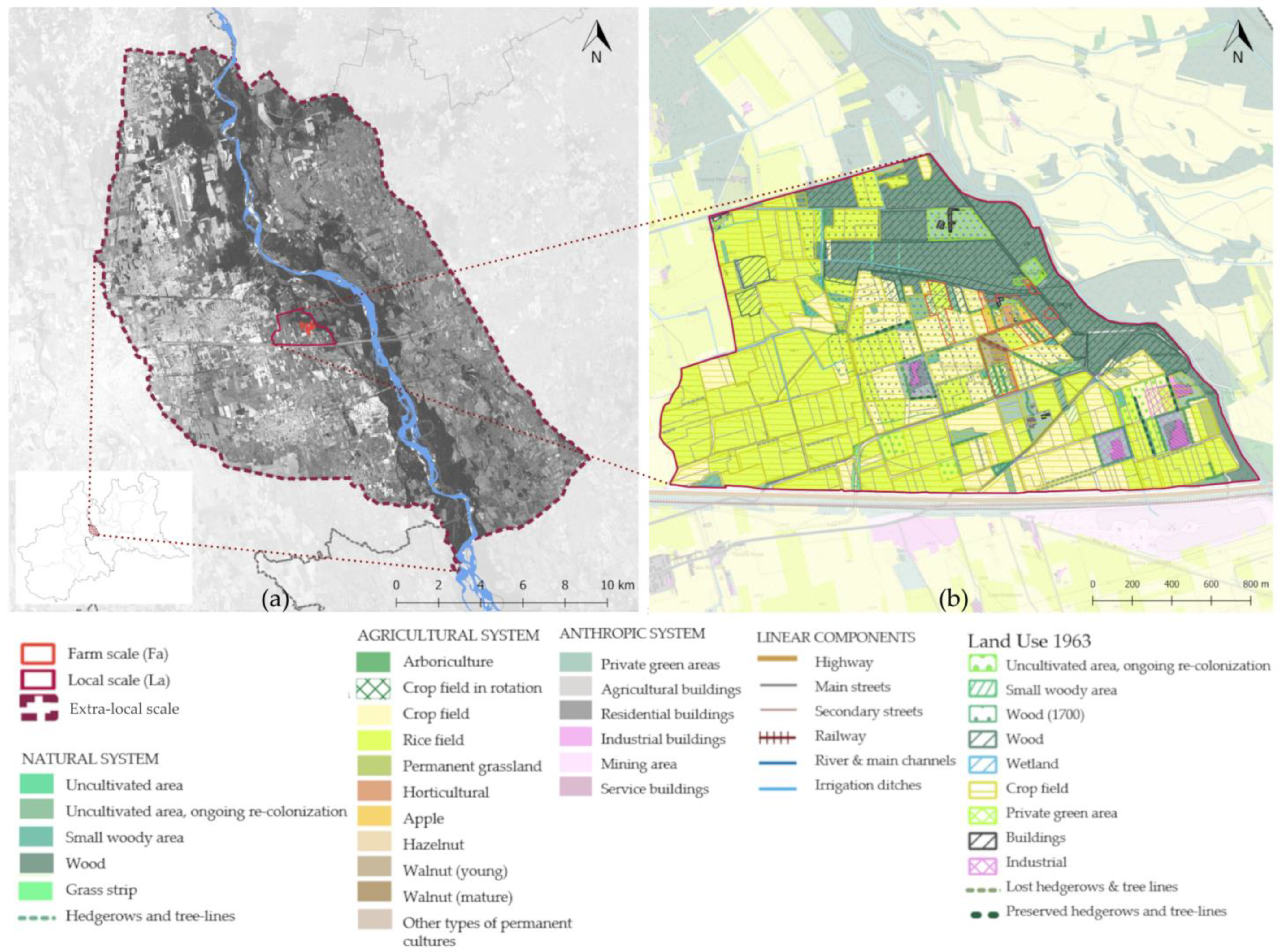
2.2. The Pilot Case Study: Environmental Context

The pilot case study on which the set of indicators was tested is an organic farm located on fluvial and fluvioglacial Würm deposits among the western Po Plain basin (Piedmont Region), nearby the Ticino River protected ecological corridor, in an agricultural context dominated by intensive conventional rice and corn production (Figure 1). This small-size pilot farm (about 13 ha) is characterized by highly diversified annual productions, under 3 years rotations (rice, barley, corn, leguminous plants, mixed horticulture), and permanent fruit productions (walnut, nut, apple). Traditional management practices are adopted, compliant with organic agriculture requirements, including the use of landraces, avoiding the use of chemical fertilizers and herbicides, recovering ancient small-sized plot texture, and the preservation and restoration of the ecological infrastructure through landscape features management (hedgerows, tree lines, riparian vegetation along irrigation ditches, wooded areas, and wooded patches).

Bioclimatically, the area belongs to the temperate oceanic (submediterranean) bioclimate, the upper meso-temperate thermotype, and the lower humid ombrotype [96,97]. The real potential vegetation is represented by the “Neutroacidophilous series of European oak and hornbeam in the lower western Po Valley” [98,99,100]. Historical land use traits (IGM 1963 [86]; and an ancient XVIII century map by the Turin State Archives) (Figure 1) highlight the long-term stability of wooded contexts, the contraction of some other wooded areas, and the progressive dismantling of the linear landscape features system. Current phytocoenoses are significantly influenced by synanthropic secondary dynamisms, especially the more unstable ones (wood margins, hedgerows, and young small wooded areas). The local flora, currently under study by the authors, is composed of 132 taxa (species and sub-species), belonging to 49 taxonomic families, mainly hemicryptophytes and therophytes and, secondarily, phanerophytes, and then geophytes, reflecting bioclimatic conditions and a variety of open and wooded habitats with different degrees of disturbance. Eurasian macro-chorotypes predominate, as expected given the biogeographic context, and species with a wide distribution in relation to anthropization. This also results in a significant presence of allochthonous species; in fact, 27.48% of the total flora is represented by allochthonous species, of which 75% are invasive exotics, while the Italian national average is 19.49% [101].

3. Results and Discussion

3.1. Landscape Ecology Analyses Results

Extra-local spatial-qualitative VR assessment (Figure 2) helped in contextualizing the pivotal buffering and permeating role that the local scale context and the pilot farm area can play, being located at the interface between a wide, protected primary ecological corridor axis and the surrounding, more simplified Po Plain agricultural context. In such a context, rural landscape features and equipment can positively spread the biotic exchanges from the neighboring source areas, broadening their effects on west-east axes through the activation of new ecological corridors. In parallel, NBFS implementation can contribute to buffering the sink effects and pollutants’ impacts coming from the agricultural matrix and major infrastructures affecting the ecological quality of the main fluvial ecological corridor.

The local scale preliminary functional variability revealed through the spatial-quantitative assessment of landscape physiological apparatuses (Figure 3a,b) highlighted a relatively good balance of stabilization and protective functions (19.8% and 5.5% of total surface, respectively). In contrast, connective functions appear to be underrepresented (1.6%), reflecting the bipolar configuration of the area, where areas with high metastability behavior (the northeastern wooded protected areas) are poorly permeated by the agricultural ones, and buffering functions between the two systems are underexpressed. The low-represented resilience functions (2.4%), performed by low-developed secondary recolonization contexts, reflect the medium disturbance level on semi-natural patches external to the more consistent stabilizing wooded patches and, in parallel, represent a potential driver of change, if properly managed. As a result, the current impact of agricultural management disturbances on floral-vegetational ecological and dynamic phytocoenoses of the agricultural system is expected, with a notable difference in wooded area traits.

3.1.1. Landscape Structural Indicators Results

Fa represents 3.7% of the total La area, 6.8% of the total La perimeter, and 11.3% of the total La number of patches. This relation already suggests higher total shape complexity for Fa (a higher total perimeter/area ratio), with smaller patches.

Results on shape indices (

Table 2. Results on landscape structural indicators [Shape Indices (NP: number of patches; MPS: Medium patches size; MTX: Matrix; MPAR: Mean Perimeter area ratio; SI: Shape index; MSI: Mean Shape index; AWSI: Area weighted mean shape index; PFD: Patch fractal dimension; MPFD: Mean patch fractal dimension; and AWPFD: Area weighted mean patch fractal dimension) and Composition Indices (DIV1a: Diversity_1a/tot; DIV1b: Diversity_1b/landscape element; DIV2: Diversity_2; DOM1: Dominance_1; DOM2: Dominance_2; LSD1: Landscape Structural Diversity_1; LSD2: Landscape Structural Diversity_2)], comparing local (La) and farm (Fa) scale levels of analysis, respectively for the natural (NAT), agricultural (AGR), and anthropic (ANT) landscape sub-systems and for the total landscape system (TOT) (in bold), for which the difference between Fa and La is shown (GAP) (see Appendix A; Table A1 for details on the studied indicators)].

		Patches Metrics			Shape Indices									Composition Indices
	Landscape Sub-system	Area [ha]	Perimeter [m]	NP	MPS	MTX	MPAR	SI	MSI	AWSI	PFD	MPFD	AWPFD	DIV1a	DIV1b	DIV2	DOM1	DOM2	LSD1	LSD2
La	NAT	76.6	25,587	49	1.12	23.5	0.010	8.2	0.47	5.4	1.50	0.16	1.46	0.5	0.6	0.2	2.4	0.8	2.6	0.6
	AGR	226.8	108,378	273	0.53	69.6	0.002	20.3	0.16	13.8	1.58	0.05	1.56	0.8	0.8	0.3	2.0	0.7	4.3	1.1
	ANT	22.2	13,886	41	0.43	6.8	0.009	8.3	0.39	6.1	1.55	0.15	1.52	0.2	0.7	0.1	2.7	0.9	1.3	0.3
	TOT	325.6	147,850	363	0.67	100.0	0.004	23.1	0.23	11.3	1.59	0.07	1.53	1.5		0.54	1.34	0.46	6.72	1.85
Fa	NAT	1.05	1315	7	0.14	8.7	0.046	3.6	0.74	3.0	1.55	0.44	1.53	0.2	0.4	0.1	2.2	0.9	1.3	0.4
	AGR	10.24	7375	26	0.43	85.2	0.021	6.5	0.64	2.9	1.54	0.39	1.46	1.6	1.7	0.7	0.8	0.3	6.0	2.2
	ANT	0.73	1382	8	0.09	6.1	0.047	4.6	0.80	3.3	1.63	0.40	1.60	0.2	0.7	0.1	2.2	0.9	1.1	0.3
	TOT	12.02	10,071	41	0.32	100.0	0.031	8.2	0.68	3.0	1.58	0.40	1.47	2.0		0.84	0.37	0.16	6.83	2.66
GAP (Fa−La)	TOT				−0.36		0.026	−14.9	0.46	−8.29	−0.01	0.33	−0.06	0.48		0.31	−0.97	−0.31	0.11	0.81
	NAT%				−88%	−63%	338%	−56%	57%	−45%	4%	181%	5%	−48%	−35%	−38%	−11%	7%	−51%	−37%
	AGR%				−19%	22%	801%	−68%	299%	−79%	−3%	704%	−6%	86%	98%	124%	−59%	−51%	41%	102%
	TOT%				−53%	0%	623%	−65%	201%	−74%	−1%	438%	−4%	31%		58%	−72%	−66%	2%	44%

and

Table 3. Correlation coefficients matrixes for shape indices (MPAR: Mean Perimeter area ratio; SI: Shape index; MSI: Mean Shape index; AWSI: Area weighted mean shape index; PFD: Patch fractal dimension; MPFD: Mean patch fractal dimension; and AWPFD: Area weighted mean patch fractal dimension) and for composition indices (DIV1a: Diversity_1a /tot; DIV1b: Diversity_1b /landscape element; DIV2: Diversity_2; DOM1: Dominance_1; DOM2: Dominance_2; LSD1: Landscape Structural Diversity_1; and LSD2: Landscape Structural Diversity_2).

	Shape Indices								Composition Indices
	MPAR	SI	MSI	AWSI	PFD	MPFD	AWPFD		DIV1a	DIV1b	DIV2	DOM1	DOM2	LSD1	LSD2
MPAR	1.00							DIV1a	1.00
SI	−0.76	1.00						DIV1b	0.94	1.00
MSI	0.93	−0.89	1.00					DIV2	0.99	0.96	1.00
AWSI	−0.76	0.94	−0.94	1.00				DOM1	−0.95	−0.89	−0.97	1.00
PFD	0.31	0.23	0.08	0.20	1.00			DOM2	−0.99	−0.96	−1.00	0.97	1.00
MPFD	0.91	−0.82	0.96	−0.89	0.12	1.00		LSD1	0.98	0.89	0.95	−0.88	−0.95	1.00
AWPFD	0.26	0.19	−0.06	0.33	0.80	−0.09	1.00	LSD2	1.00	0.95	1.00	−0.97	−1.00	0.96	1.00

; Figure 4) highlighted the following traits (see Appendix A; Table A1 for details on the studied indicators):

• Positively lower MPS values for Fa (MPS equal to 0.43 ha; −19% for the AGR Fa sub-system), which reflect the positive effects related to small-sized agricultural patches among the pilot farm: higher landscape heterogeneity [102,103]; hedge microhabitat and niche diversification [104,105,106]; lower sink effects [54,107]; increased variability of micro-climatic conditions and provision of breeding sites [108,109]; and encouraging species diversification and higher avian diversity (a balance between generalist and specialist behaviors) [54,110,111,112];
• Relatively high MPS values for the La NAT sub-system (MPS equal to 1.12 ha) reflect a proper consistency of natural (woody) patches among La. This can be related to a positive influence on the properties of source areas: interior habitat conditions, higher specialist species population sizes, lowering their probability of local extinction, rising stability traits, and balancing the impacts coming from the neighboring agricultural matrix [13,54]. These traits underline the current pivotal role of the existing woody components and the potential that could be displayed by their preservation, proper management (improvement of their ecological quality), and extension;
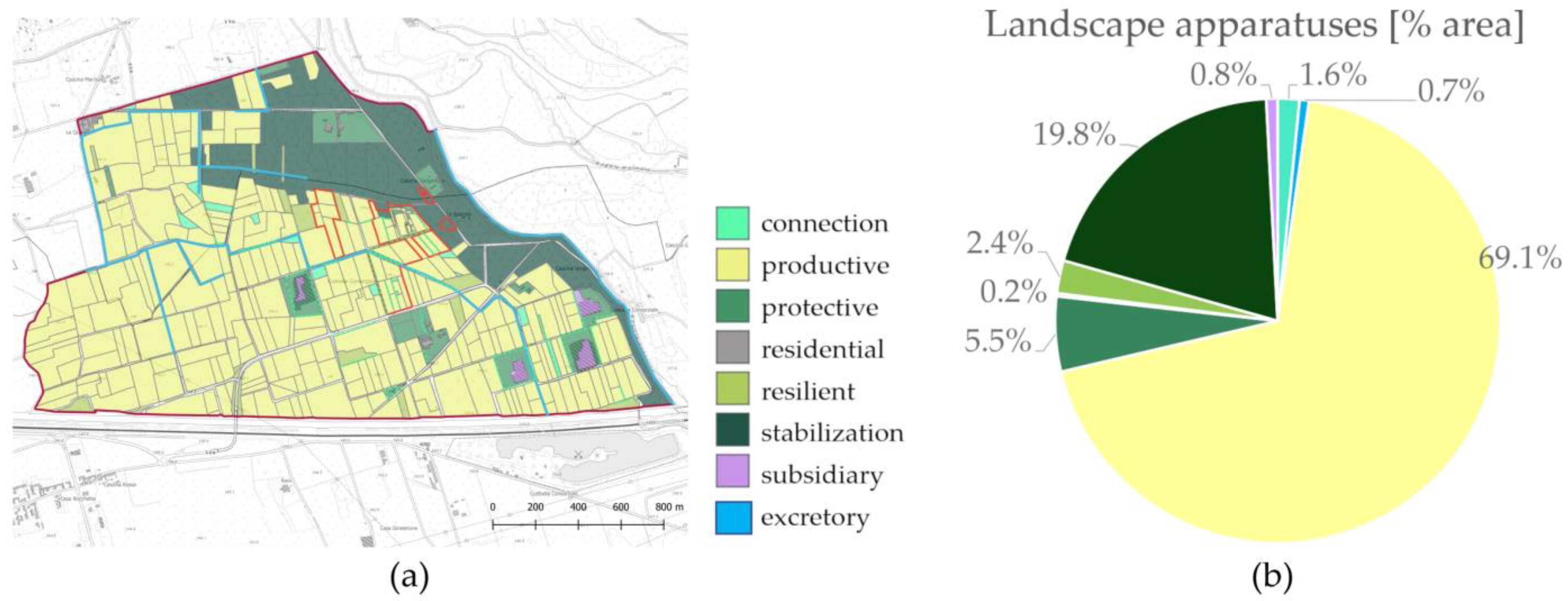
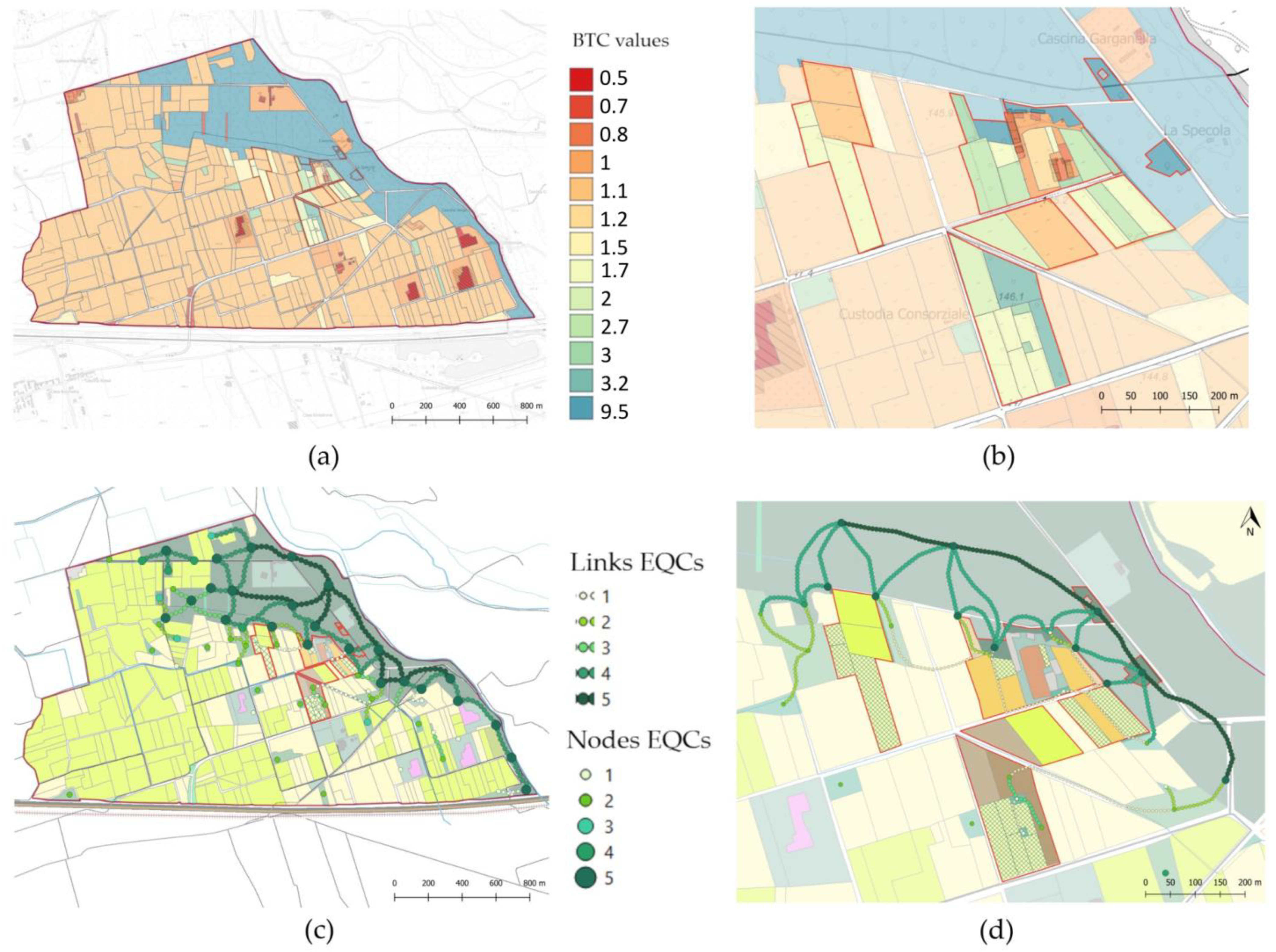
• The MTX index showed, as expected: lower occurrence of natural sub-system components in Fa (−63%), which might be enhanced through the further integration of diffused natural and semi-natural components and in between productive fields [102,104,105]; higher relative occurrence in Fa of agricultural sub-system components (+22%); and good stability of the La agricultural matrix (absence of significantly spread impacts derived from non-compatible land uses) (69.6% of total surface), as it was already highlighted by landscape apparatus analysis (Figure 3a,b). This increases the potential for effectively correcting the current ecological trends toward higher quality values [13,113,114,115];
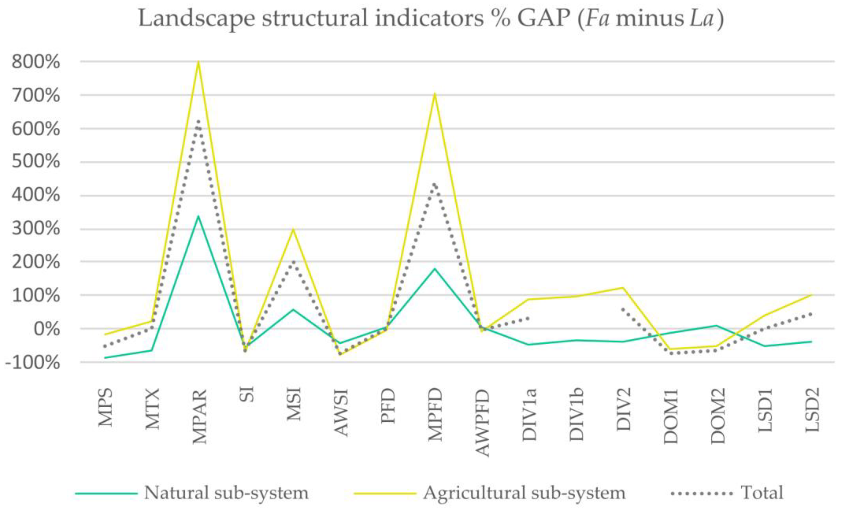
• Indices related to patch shape complexity (MPAR, SI, PFD, and their variants) showed positive results (significantly higher patch complexity) for Fa in their arithmetic mean variants, where the effect of the different Fa and La overall dimensions is kept under control (average single patch values): MPAR (+623% in TOT Fa), MSI (+201% in TOT Fa), and MPFD (+438% in TOT Fa). Thus, MPAR, MSI, and MPFD showed good sensitivity to La and Fa differences. They were also positively correlated (Table 3) and can be consequently considered redundant in the studied context (they capture similar qualities of spatial patterns); their potential interchange might be further tested among larger datasets. In contrast, their area-weighted mean variants (AWSI and AWPFD) showed negative results for Fa. This was influenced by the over-weighting of agricultural patches on wider surfaces in La, while the narrow, small-sized, elongated agricultural patches in Fa were down-weighted by the algorithm. These effects are widened by differences in the overall dimensions of La and Fa, implying that such area-weighted indices are unsuitable for comparing different scale contexts. Further testing of such indicators in equally-sized contexts would integrate such assumptions [59]. PFD values showed relative low sensitivity to Fa and La differences (−3% in AGR Fa and −1% in TOT Fa) compared to the other shape complexity indicators. Its suitability for project purposes should be further checked on wider datasets. Shape complexity in agricultural contexts is suitable for representing the level of patch inter-digitation: high values inform on ecological exchange trends (high exposure to neighboring impacting land uses or high permeability to biotic and resource exchanges with neighboring semi-natural land uses). Thus, their positive or negative ecological value interpretation should be paired with context ecological quality analysis, such as landscape apparatuses and BTC values spatial variability analysis. For instance, among Fa, shape complexity values should be interpreted as positively supporting the NBFS effects as well as the exchanges with the neighboring wooded areas (even if critical exposure to neighboring conventional patches should be considered as well). Moreover, if intended as a measure of land use intensity [69], positive values of shape complexity indices can be indirectly related to heterogeneity and diversity values, especially in rural contexts (checkerboard-shaped landscapes) [55,69,116,117,118].

Results on landscape composition indices (DIV_[1a-1b-2], DOM _[1–2], and LSD _[1–2]) (Table 2 and Table 3, Figure 4) highlighted the following traits:

• Among landscape diversity indicators, both DIV_[1a-1b-2] showed relative positive contributions of Fa to the agricultural sub-system heterogeneity (+86%, +98%, and +124% in AGR Fa, respectively). Both DIV_[1a-2] showed positive contributions of Fa to the total landscape system diversification, while lower values were registered for the Fa natural sub-system diversity (both for DIV_[1a-1b-2]), highlighting the need for further improvement of natural landscape features and their configuration in the pilot case study in order to better counterbalance its positive contributions towards the surrounding context. DIV₂ showed the highest relative sensitivity to changes (both for the agricultural subsystem and for the total area), and it should be considered to have higher congruency as it is a normalized version of DIV_1a and its values do not depend on the number of land use categories, being more independent of scale [59];
• As expected, DOM _[1–2] indicators are inversely correlated to DIV_[1a-1b-2] ones (Table 3), and consequently provide redundant information. They were the basis for computing LSD _[1–2] values, which showed a positive contribution of Fa to the agricultural sub-system diversification [respectively, +41% (LSD₁) and +102% (LSD₂) in AGR Fa]. In comparison, the total landscape system LSD _[1–2] showed smaller changes (+2% and +44% in TOT Fa, respectively), with LSD₂ showing a higher relative sensitivity to changes between total La and Fa, in line with the trend between DIV_1a-2 indicators. In line with all DIV_[1a-1b-2] values, higher LSD _[1–2] values were registered for the La on a natural sub-system (LSD₁ −51% for NAT Fa and LSD₂ −37% for NAT Fa), confirming the above-cited DIV_[1a-1b-2] value interpretation;
• All DIV_[1a-1b-2] and LSD _[1–2] indicators are positively correlated between each other (Table 3), consequently bringing redundant information, as was expected, and suggesting the opportunity of their screening. Indeed, they were included to allow the comparison of their different performances (a preliminary assessment of their sensitivity to changes among the different studied contexts).

Taken together, landscape composition indices, representing landscape heterogeneity values, showed good relative sensitivity to La and Fa agricultural and natural sub-system differences, which should be further tested on wider datasets for a comprehensive and coherent sensitivity screening. The dependence of the different indicators on other spatial factors should also be taken into account (first of all, changes in the scale of analysis). Especially, the DIV₂ and LSD₂ indices were found to be good informative metrics and appeared to be the most suitable ones for fitting the study purposes.

The highlighted positive contribution of Fa to AGR and TOT landscape heterogeneity supports the hypothesis of the contribution given by NBFS approaches to agroecosystem diversification, supporting the following related functions among rural land:

• Higher habitat diversification enables source populations to spillover from semi-natural patches to intensively managed patches, balancing generalist and specialist species presences, rising species richness values of different taxa, and reducing local extinction risks [70,102,104,105,111,119,120,121,122,123,124,125,126];
• Activation of buffering functions at the natural-agricultural fringe, moderating the impacts derived from intensive local land use through diversified diachronic micro-habitat provisioning (source and refuge areas) [54,103].

As a whole, the results on landscape structural indicators were useful in underlying the contributions given by the pilot farm’s NBFS-oriented approach to landscape diversification, buffering the negative effects on structural and functional biodiversity values derived from the oversimplification patterns that characterise conventional agricultural landscape ecological systems.

3.1.2. Landscape Functional Indicators Results

In line with landscape apparatus analysis, BTC values of spatial distribution (Figure 5a,b) highlight the relative high contribution given by woody patches to the overall meta-stability of the studied context, whereas the agricultural matrix shows a significant absence of inter-spread positive BTC values components, except for a central area where the pilot farm is also located. Indeed, the BTC analysis underlined the positive contribution given by the diversified (over space and time scales) land uses among the pilot farm, which represents a unicum among the agricultural matrix. This highlights the potential contribution of widespread implementation of NBFS to the release of higher metastability values across rural land outside natural areas, which could positively enhance the homeostatic and homeorhetic capacities of this agricultural system and, consequently, its resistance and adaptation capacities. These statements are aligned with the results obtained on the other structural and functional landscape ecology indices.

The analysis of functional connectivity (CON and WCON) and circuitry (CIR and WCIR) indicators (Figure 5c,d) showed good relative sensitivity, with parallel trends between the Fa and La scales. Results confirm the role of the local scale northeastern woody patches in sustaining the biotic and abiotic fluxes across the landscape system, whereas the low NBFS equipment of the agricultural matrix significantly lowers the overall local scale connectivity and circuitry values. The comparison of the CON and CIR indices between the La and Fa scales (Figure 6a) highlights the positive contribution on ecological fluxes given by NBFS implementation among the pilot farm (+0.13 on CON; +0.18 on CIR). Indeed, connectivity functions are tightly related to population and metapopulation dynamics and biodiversity values [13,54,113,127,128,129,130,131,132,133]. The indices’ weighted variants (WCON and WCIR) allowed us to efficiently take into account the role of the effective current ecological status of connectivity components (links), highlighting the distance from optimal conditions and counterbalancing the negative connectivity effects related to generalist species’ predisposition to low EQC corridors [134,135]. Indeed, the WCON and WCIR index values show smaller discrepancies between La and Fa scales (+ 0.06 on the Fa WCON and + 0.08 on the Fa WCIR, respectively), a result related to the current medium to low ecological quality of the linear landscape features among the pilot farm, which, despite being relatively spread, could benefit from further ecological requalification. In line with this, the distribution of La and Fa scale links among the different EQC_y (Figure 6b) shows mixed patterns, with low-EQC_y links being more represented among Fa scale (+7% on the 1st EQC and +4% on the 2nd EQC) and a higher percentage of the maximum EQC_y at La scale (+6% on the 5th EQC), where connectivity functions are mostly expressed by high ecological quality woody patches. These results suggest a good suitability of the EQC synthetic weighting system for monitoring slight changes over time.

In line with these results, the landscape apparatus analysis revealed low connectivity functions throughout the overall La context. Their spread across the agricultural matrix would be pivotal in any corrective management strategy, as was highlighted through the extra-local and local VR analyses.

The local scale VR analysis (Figure 7), as a conceptual result of multiple territorial information overlays and landscape ecology analyses, gives a synthetic qualitative outline of the predominant spatial configuration of ecological fluxes of information, genetic, trophic, and biotic resources across the La scale area. Such an analysis shows the positive current and potential contribution that the pilot farm under study can make in relation to its surrounding context. The current synthesis helps in prioritizing the featuring and allocation of the ecological reconfiguring strategies as a response to the criticalities highlighted by the landscape ecology analyses, which are currently impacting floristic-vegetational ecological quality and agrobiodiversity values (low connectivity and circuitry levels among the agricultural matrix, over-sized patches acting as source areas, relative low spatial heterogeneity, barrier effect derived from major infrastructures) (see Section 3.1.1 and Section 3.1.2). The strategic mending and buffering role of the agricultural areas neighboring the wooded areas (where the pilot farm is also located) are highlighted.

4. Conclusions

The results presented in this study were based on a workflow that was intended to examine different facets of the ecological functions and processes that interact among agroecosystems. The study allows the preliminary selection and screening of the most sensitive and informative analyses to be integrated into an NBFS assessment methodology in which analytical steps are closely interlinked with management practice targeting and farmland ecological design strategic orientation. Multi-scale evaluations, with different levels of detail, were useful for representing the inter-linkages existing between farm-scale ecological traits and the surrounding local landscape context, which is influenced by and influences the surrounding extra-local landscape system ecological configuration (more detailed analyses).

The results of the Fa and La scale levels of analysis allow for the identification of the main ecological traits associated with the pilot farm NBFS management, demonstrating its positive contributions when compared to the business as usual conventionally managed surrounding La scale context. The ecological interpretation is based on the acknowledged role of landscape metrics as surrogates for agrobiodiversity values. Nonetheless, the in-view comparison of landscape metrics results with multi-scale floristic-vegetational indicators assessment would broaden the ecological interpretation, allowing an examination of the use of landscape metrics as correlates of agrobiodiversity indices, screening and validating their value as context-specific agrobiodiversity proxies.

From a methodological point of view, this study helps in preliminarily identifying a set of indicators suitable for the multi-scale assessment of NBFS contributions to agrobiodiversity in the studied pedo-climatic context. High sensitivity to different management options, low redundancy, and good suitability for multi-scale comparisons were the guiding evaluation criteria. Further research on larger datasets derived from other pilot case studies with similar pedo-climatic conditions is required to improve the statistical consistency of the methodology presented here. In particular, the comparison of pilot case studies with conventional farms at the same scale (Fa) would allow a finer screening of the most suitable indicators, integrating the preliminary results better by considering the sensitivity of the indicators to changes in scales of analysis.

Overall, the results presented in this study are expected to provide new useful tools that can be applied to farming systems belonging to similar pedo-climatic conditions and integrate current knowledge on synthetic agrobiodiversity indicators.

Moreover, this multi-scale approach appeared to be suitable for interlinking best-practice assessments (a result-based monitoring approach) with effective best-practice promotion and spread (a science-driven strategic NBFS design approach). Indeed, current ecosystem functions supported by the NBFS were interlinked with potential future enhancements of ecosystem functions through VR analysis. Such an approach paves the way for integrating the ecosystem functions and services approach into the assessment and design processes, both on a spatial-qualitative and quantitative basis [136,137,138,139,140,141].

References

- Altieri, M.A. The ecological role of biodiversity in agroecosystems. Agric. Ecosyst. Environ. 1999, 74, 19–31. [Google Scholar] [CrossRef] [Green Version]
- Benton, T.G. Managing Farming’s Footprint on Biodiversity. Science 2007, 315, 341–342. [Google Scholar] [CrossRef] [PubMed]
- Fabbri, P. Natura e Cultura del Paesaggio Agrario, Indirizzi per La Tutela e la Progettazione; Città Studi Edizioni: Milan, Italy, 1997. [Google Scholar]
- Gliessman, S.R. Agroecology: The Ecology of Sustainable Food Systems, 2nd ed.; Taylor & Francis Group, Ed.; CRC Press: Boca Raton, FL, USA, 2007. [Google Scholar]
- Miralles-Wilhelm, F.; Iseman, T. Nature-Based Solutions in Agriculture—The Case and Pathway for Adoption; Food & Agriculture Org. and The Nature Conservancy: Arlington, VA, USA, 2021. [Google Scholar] [CrossRef]
- Wojtkowski, P. Landscape Agroecology, 1st ed.; CRC Press: Boca Raton, FL, USA, 2003. [Google Scholar]
- Altieri, M.A. Agroecology: The Scientific Basis of Alternative Agriculture; Division of Biological Control, University of California: Berkeley, CA, USA, 1983. [Google Scholar]
- Jackson, L.E.; Pascual, U.; Hodgkin, T. Utilizing and conserving agrobiodiversity in agricultural landscapes. Agric. Ecosyst. Environ. 2007, 121, 196–210. [Google Scholar] [CrossRef]
- Oliver, T.H.; Heard, M.S.; Isaac, N.J.B.; Roy, D.B.; Procter, D.; Eigenbrod, F.; Freckleton, R.; Hector, A.; Orme, C.D.L.; Petchey, O.L.; et al. Biodiversity and Resilience of Ecosystem Functions. Trends Ecol. Evol. 2015, 30, 673–684. [Google Scholar] [CrossRef] [PubMed] [Green Version]
- Kremen, C.; Merenlender, A.M. Landscapes that work for biodiversity and people. Science 2018, 362. [Google Scholar] [CrossRef] [Green Version]
- Tscharntke, T.; Klein, A.; Kruess, A.; Steffan-Dewenter, I.; Thies, C. Landscape perspectives on agricultural intensification and biodiversity—Ecosystem service management. Ecol. Lett. 2005, 8, 857–874. [Google Scholar] [CrossRef]
- Tilman, D.; Isbell, F.; Cowles, J.M. Biodiversity and Ecosystem Functioning. Annu. Rev. Ecol. Evol. Syst. 2014, 45, 471–493. [Google Scholar] [CrossRef]
- Donald, P.F.; Evans, A.D. Habitat connectivity and matrix restoration: The wider implications of agri-environment schemes. J. Appl. Ecol. 2006, 43, 209–218. [Google Scholar] [CrossRef]
- Hooper, D.U.; Chapin Iii, F.S.; Ewel, J.J.; Hector, A.; Inchausti, P.; Lavorel, S.; Lawton, J.H.; Lodge, D.M.; Loreau, M.; Naeem, S.; et al. Effects of biodiversity on ecosystem functioning: A consensus of current knowledge. Ecol. Monogr. 2005, 75, 3–35. [Google Scholar] [CrossRef]
- Opdam, P.; Wascher, D. Climate change meets habitat fragmentation: Linking landscape and biogeographical scale levels in research and conservation. Biol. Conserv. 2004, 117, 285–297. [Google Scholar] [CrossRef]
- Chapin, F.S., III; Zavaleta, E.S.; Eviner, V.T.; Naylor, R.L.; Vitousek, P.M.; Reynolds, H.L.; Hooper, D.U.; Lavorel, S.; Sala, O.E.; Hobbie, S.E.; et al. Consequences of changing biodiversity. Nature 2000, 405, 234–242. [Google Scholar] [CrossRef] [PubMed]
- Oliveira, B.F.; Moore, F.C.; Dong, X. Biodiversity mediates ecosystem sensitivity to climate variability. Commun. Biol. 2022, 5, 628. [Google Scholar] [CrossRef] [PubMed]
- Hulme, P.E. Adapting to climate change: Is there scope for ecological management in the face of a global threat? J. Appl. Ecol. 2005, 42, 784–794. [Google Scholar] [CrossRef]
- Honnay, O.; Verheyen, K.; Butaye, J.; Jacquemyn, H.; Bossuyt, B.; Hermy, M. Possible effects of habitat fragmentation and climate change on the range of forest plant species. Ecol. Lett. 2002, 5, 525–530. [Google Scholar] [CrossRef]
- Grime, J.P.; Brown, V.K.; Thompson, K.; Masters, G.J.; Hillier, S.H.; Clarke, I.P.; Askew, A.P.; Corker, D.; Kielty, J.P. The Response of Two Contrasting Limestone Grasslands to Simulated Climate Change. Science 2000, 289, 762–765. [Google Scholar] [CrossRef]
- Hernández-Morcillo, M.; Burgess, P.; Mirck, J.; Pantera, A.; Plieninger, T. Scanning agroforestry-based solutions for climate change mitigation and adaptation in Europe. Environ. Sci. Policy 2018, 80, 44–52. [Google Scholar] [CrossRef] [Green Version]
- Maes, J.; Jacobs, S. Nature-Based Solutions for Europe’s Sustainable Development. Conserv. Lett. 2017, 10, 121–124. [Google Scholar] [CrossRef] [Green Version]
- European Commission. Communication from the Commission to the European Parliament, the Council, the European Economic and Social Committee and the Committee of the Regions, Green Infrastructure (GI)-Enhancing Europe’s Natural Capital {SWD(2013) 155 Final}. 2013, COM(2013) 249 Final. Available online: https://eur-lex.europa.eu/legal-content/EN/TXT/?uri=celex%3A52013DC0249 (accessed on 5 January 2023).
- European Commission. Towards an EU Research and Innovation Policy Agenda for Nature-Based Solutions & Re-Naturing Cities: Final Report of the Horizon 2020 Expert Group on ‘Nature-Based Solutions and re-Naturing Cities’: (Full Version); Publications Office, Directorate-General for Research and Innovation: Brussels, Belgium, 2015.
- European Commission. Communication from the Commission to the European Parliament, the European Council, the Council, the European Economic and Social Committee and the Committee of the Regions—The European Green Deal. 2019, 11.12.2019 COM(2019) 640 final. Available online: https://eur-lex.europa.eu/legal-content/EN/TXT/?uri=COM%3A2019%3A640%3AFIN (accessed on 5 January 2023).
- European Commission. Communication from the Commission to the European Parliament, the Council, the European Economic and Social Committee and the Committee of the Regions—A Farm to Fork Strategy. 2020, 20.05.2020 COM (2020) 381 final. Available online: https://eur-lex.europa.eu/legal-content/EN/TXT/?uri=CELEX%3A52020DC0381 (accessed on 5 January 2023).
- European Commission. List of Potential Agricultural Practices That Eco-Schemes could Support; European Commission: Brussels, Belgium, 2021. Available online: https://agriculture.ec.europa.eu/news/commission-publishes-list-potential-eco-schemes-2021-01-14_en#moreinfo (accessed on 5 January 2023).
- United Nations. Transforming Our World: The 2030 Agenda for Sustainable Development, Resolution Adopted by the General Assembly on 25 September 2015; United Nations: San Francisco, CA, USA, 2015; A/RES/70/1.
- MEA. Ecosystems and Human Well-Being—Synthesis, Millennium Ecosystem Assessment; Island Press: Washington, DC, USA, 2005; Volume A/RES/70/1. [Google Scholar]
- AAVV. Towards Integrating Biological and Landscape Diversity for Sustainable Agriculture in Europe. In Proceedings of the High-Level Pan-European Conference on Agriculture and Biodiversity, Paris, France, 5–7 June 2002. [Google Scholar]
- Evans, A.D.; Armstrong-Brown, S.; Grice, P.V. The role of research and development in the evolution of a ‘smart’ agri-environment scheme. Asp. Appl. Biol. 2002, 67, 253–262. [Google Scholar]
- Kleijn, D.; Berendse, F.; Smit, R.; Gilissen, N. Agri-environment schemes do not effectively protect biodiversity in Dutch agricultural landscapes. Nature 2001, 413, 723–725. [Google Scholar] [CrossRef]
- Kleijn, D.; Berendse, F.; Smit, R.; Gilissen, N.; Smit, J.; Brak, B.; Groeneveld, R. Ecological Effectiveness of Agri-Environment Schemes in Different Agricultural Landscapes in The Netherlands. Conserv. Biol. 2004, 18, 775–786. [Google Scholar] [CrossRef]
- Krebs, J.R.; Wilson, J.D.; Bradbury, R.B.; Siriwardena, G.M. The second Silent Spring? Nature 1999, 400, 611–612. [Google Scholar] [CrossRef]
- Herzon, I.; Birge, T.; Allen, B.; Povellato, A.; Vanni, F.; Hart, K.; Radley, G.; Tucker, G.; Keenleyside, C.; Oppermann, R.; et al. Time to look for evidence: Results-based approach to biodiversity conservation on farmland in Europe. Land Use Policy 2018, 71, 347–354. [Google Scholar] [CrossRef]
- Burton, R.J.F.; Schwarz, G. Result-oriented agri-environmental schemes in Europe and their potential for promoting behavioural change. Land Use Policy 2013, 30, 628–641. [Google Scholar] [CrossRef] [Green Version]
- Nitsch, H.; Bogner, D.; Dubbert, M.; Fleury, P.; Hofstetter, P.; Knaus, F.; Rudin, S.; Šabec, N.; Schmid, O.; Schramek, J.; et al. MERIT. Review on Result-Oriented Measures for Sustainable Land Management in Alpine Agriculture & Comparison of Case Study Areas. Report of Work Package 1. RURAGRI Res. Programme 2013–2016; European Commission: Luxembourg, 2014.
- Keenleyside, C.; Radley, G.; Tucker, G.; Underwood, E.; Hart, K.; Allen, B.; Menadue, H. Results-Based Payments for Biodiversity Guidance Handbook: Designing and Implementing Results-Based Agri-Environment Schemes 2014-20, Prepared for the European Commission, DG Environment; Institute for European Environmental Policy: London, UK, 2014; Volume Contract No ENV.B.2/ETU/2013/0046. [Google Scholar]
- Underwood, E. Results-Based Payments for Biodiversity, Supplement to Guidance Handbook, Result Indicators Used in Europe, the Selection, Testing Measurement and Verification of Indicators of Biodiversity Results, Prepared for the European Commission, DG Environment; Institute for European Environmental Policy: London, UK, 2014; Volume Contract No ENV.B.2/ETU/2013/0046. [Google Scholar]
- Stolze, M.; Frick, R.; Schmid, O.; Stöckli, S.; Bogner, D.; Chevillat, V.; Dubbert, M.; Fleury, P.; Neuner, S.; Nitsch, H.; et al. Result-Oriented Measures for Biodiversity in Mountain Farming—A Policy Handbook; Researc Institute of Organic Agriculture (FiBL): Frick, Switzerland, 2015. [Google Scholar]
- Schröder, S.; Begemann, F.; Harrer, S. Agrobiodiversity monitoring—Documentation at European level. J. Für Verbrauch. Und Lebensm. 2007, 2, 29–32. [Google Scholar] [CrossRef]
- Taffetani, F.; Rismondo, M. Bioindicators system for the evaluation of the environment quality of agro-ecosystems. Fitosociologia 2009, 46, 3–22. [Google Scholar]
- Taffetani, F.; Rismondo, M.; Lancioni, A. Integrated tools and methods for the analysis of agro-ecosystem’s functionality through vegetational investigations. Fitosociologia 2011, 48, 41–52. [Google Scholar]
- Bassignana, C.F.; Merante, P.; Belliére, S.R.; Vazzana, C.; Migliorini, P. Assessment of Agricultural Biodiversity in Organic Livestock Farms in Italy. Agronomy 2022, 12, 607. [Google Scholar] [CrossRef]
- Tasser, E.; Rüdisser, J.; Plaikner, M.; Wezel, A.; Stöckli, S.; Vincent, A.; Nitsch, H.; Dubbert, M.; Moos, V.; Walde, J.; et al. A simple biodiversity assessment scheme supporting nature-friendly farm management. Ecol. Indic. 2019, 107, 105649. [Google Scholar] [CrossRef] [Green Version]
- Duelli, P.; Obrist, M.K. Biodiversity indicators: The choice of values and measures. Agriculture, Ecosystems & Environment 2003, 98, 87–98. [Google Scholar] [CrossRef]
- Migliorini, P.; Vazzana, C. Biodiversity Indicators for Sustainability Evaluation of Conventional and Organic Agro-ecosystems. Ital. J. Agron. 2007, 2, 105–110. [Google Scholar] [CrossRef]
- Blumetto, O.; Castagna, A.; Cardozo, G.; García, F.; Tiscornia, G.; Ruggia, A.; Scarlato, S.; Albicette, M.M.; Aguerre, V.; Albin, A. Ecosystem Integrity Index, an innovative environmental evaluation tool for agricultural production systems. Ecol. Indic. 2019, 101, 725–733. [Google Scholar] [CrossRef]
- Clergue, B.; Amiaud, B.; Pervanchon, F.; Lasserre-Joulin, F.; Plantureux, S. Biodiversity: Function and assessment in agricultural areas. Rev. Sustain. Agric. 2005, 25, 1–15. [Google Scholar] [CrossRef]
- Chase, J.M.; McGill, B.J.; Thompson, P.L.; Antão, L.H.; Bates, A.E.; Blowes, S.A.; Dornelas, M.; Gonzalez, A.; Magurran, A.E.; Supp, S.R.; et al. Species richness change across spatial scales. Oikos 2019, 128, 1079–1091. [Google Scholar] [CrossRef] [Green Version]
- Mazerolle, M.J.; Villard, M.-A. Patch characteristics and landscape context as predictors of species presence and abundance: A review1. Écoscience 1999, 6, 117–124. [Google Scholar] [CrossRef]
- Duelli, P. Biodiversity Evaluation in Agricultural Landscapes: An Approach at Two Different Scales. Agric. Ecosyst. Environ. 1997, 62, 81–91. [Google Scholar] [CrossRef]
- Dover, J.W.; Bunce, R.G.H. Key Concepts in Landscape Ecology; IALE UK, Coplin Cross Printers Ltd.: Garstang, UK, 1998. [Google Scholar]
- Dramstad, W.E.; Olson, J.D.; Forman, R.T.T. Landscape Ecology Principles in Landscape Architecture and Land Use Planning; Island Press: Washington, DC, USA, 1996. [Google Scholar]
- Forman, R.T.T. Land Mosaics: The Ecology of Landscapes and Regions, 1st ed.; Cambridge University Press: Cambridge, UK, 1995. [Google Scholar]
- Forman, R.T.T.; Godron, M. Landscape Ecology; J. Wiley and Sons: New York, NY, USA, 1986. [Google Scholar]
- Turner, M.G.; Gardner, R.H. Quantitative Methods in Landscape Ecology, the Analysis and Interpretation of Landscape Heterogeneity; Springer: New York, NY, USA, 1991. [Google Scholar]
- Urban, D.L.; O’Neill, R.V.; Shugart, H.H., Jr. Landscape Ecology, A Hierarquical Perspective Can Help Scientists Understand Spatial Patterns. BioScience 1987, 37, 119–127. [Google Scholar] [CrossRef]
- Turner, M.G.; Gardner, R.H. Landscape Ecology in Theory and Practice, Pattern and Process; Springer: New York, NY, USA, 2015. [Google Scholar]
- Wezel, A.; Casagrande, M.; Celette, F.; Vian, J.-F.; Ferrer, A.; Peigné, J. Agroecological practices for sustainable agriculture. A Review. Agron. Sustain. Dev. 2014, 34, 1–20. [Google Scholar] [CrossRef] [Green Version]
- Manning, P.; Loos, J.; Barnes, A.D.; Batáry, P.; Bianchi, F.J.J.A.; Buchmann, N.; De Deyn, G.B.; Ebeling, A.; Eisenhauer, N.; Fischer, M.; et al. Chapter Ten—Transferring biodiversity-ecosystem function research to the management of ‘real-world’ ecosystems. Adv. Ecol. Res. 2019, 61, 323–356. [Google Scholar] [CrossRef] [Green Version]
- Opdam, P.; Foppen, R.; Vos, C. Bridging the gap between ecology and spatial planning in landscape ecology. Landsc. Ecol. 2001, 16, 767–779. [Google Scholar] [CrossRef]
- Braun-Blanquet, J. Pflanzesoziologie; Springer: Wien, Austria, 1964. [Google Scholar]
- Pirola, A. Elementi di Fitosociologia; CLUEB: Bologna, Italy, 1970. [Google Scholar]
- Géhu, J.M. L’analyse symphytosociologique et géosymphytosociologique de l’espace, Théorie et métodologie. Coll. Phytosoc. 1988, 17, 11–46. [Google Scholar]
- Géhu, J.M.; Rivas-Martínez, S. Notions fondamentales de phytosociologie. In “Syntaxonomie”, Berichte der Internationalen Symposien der Internationalen Vereinigung für Vegetationskunde; Vaduz, Cramer: Rinteln, Germany, 1981; pp. 5–33. [Google Scholar]
- Rivas-Martínez, S. Nociones sobre Fitosociología, Biogeografía e Bioclimatología. In La vegetation de España; Universidad de Alcalá de Henares: Alcalá de Henares, Spain, 1987; pp. 19–45. [Google Scholar]
- Honnay, O.; Piessens, K.; Van Landuyt, W.; Hermy, M.; Gulinck, H. Satellite based land use and landscape complexity indices as predictors for regional plant species diversity. Landsc. Urban Plan. 2003, 63, 241–250. [Google Scholar] [CrossRef]
- Moser, D.; Zechmeister, H.G.; Plutzar, C.; Sauberer, N.; Wrbka, T.; Grabherr, G. Landscape patch shape complexity as an effective measure for plant species richness in rural landscapes. Landsc. Ecol. 2002, 17, 657–669. [Google Scholar] [CrossRef]
- Maskell, L.C.; Botham, M.; Henrys, P.; Jarvis, S.; Maxwell, D.; Robinson, D.A.; Rowland, C.S.; Siriwardena, G.; Smart, S.; Skates, J.; et al. Exploring relationships between land use intensity, habitat heterogeneity and biodiversity to identify and monitor areas of High Nature Value farming. Biol. Conserv. 2019, 231, 30–38. [Google Scholar] [CrossRef]
- Burel, F. Effect of landscape structure and dynamics on species diversity in hedgerow networks. Landsc. Ecol. 1992, 6, 161–174. [Google Scholar] [CrossRef] [Green Version]
- Ingegnoli, V.; Pignatti, S. The impact of the widened landscape ecology on vegetation science: Towards the new paradigm. Atti Della Accad. Naz. Dei Lincei. Rend. Lincei. Sci. Fis. E Nat. 2007, 18, 89–122. [Google Scholar] [CrossRef]
- Ingegnoli, V. The study of vegetation for a diagnostical evaluation of agricultural landscapes, some examples fom Lombardy. Ann. Bot. Nuova Ser. 2006, 6, 111–120. [Google Scholar]
- Burel, F. Hedgerows and Their Role in Agricultural Landscapes. Crit. Rev. Plant Sci. 1996, 15, 169–190. [Google Scholar] [CrossRef]
- Franco, D. Paesaggio, Reti Ecologiche ed Agroforestazione: Il Ruolo Dell’ecologia del Paesaggio e Dell’agroforestazione nella Riqualificazione Ambientale e Produttiva del Paesaggio/di Daniel Franco; Il Verde Editoriale: Milan, Italy, 2000. [Google Scholar]
- Franco, D. Ecological networks: The state of the art from a landscape ecology perspective in the national framework. In Reti Ecologiche: Una Chiave per la Conservazione e la Gestione dei Paesaggi Frammentati; Sitzia, T., Reniero, S., Eds.; Pubblicazioni del Corso di Cultura in Ecologia, Atti del XL Corso, Università degli Studi: Padova, Italy, 2004. [Google Scholar]
- Schoeman, Y. The Role of Landscape Ecology in the Management of Agroecosystems; Technical Report (Project Eco Agriculture); University of the Free State: Bloemfontein, South Africa, 2009. [Google Scholar] [CrossRef]
- Ingegnoli, V. Landscape Ecology: A Widening Foundation; Springer: Berlin/Heidelberg, Germany, 2002. [Google Scholar]
- Battisti, C. Frammentazione Ambientale, Connettività, Reti Ecologiche—Un Contributo Teorico e Metodologico con Particolare Riferimento Alla Fauna Selvatica; Provincia di Roma, Assessorato alle Politiche Agricole, Ambientali e Protezione Civile: Rome, Italy, 2004. [Google Scholar]
- Ryszkowski, L. Landscape Ecology in Agroecosystems Management; CRC Press: Boca Raton, FL, USA, 2001. [Google Scholar]
- Pignatti, S. Ecologia del Paesaggio/Sandro Pignatti; UTET: Torino, Italy, 1994. [Google Scholar]
- Ingegnoli, V. Landscape Bionomics: Biological-Integrated Lanscape Ecology; Springer: Milan, Italy, 2015. [Google Scholar]
- Ingegnoli, V.; Bocchi, S.; Giglio, E. Landscape Bionomics: A Systemic Approach to Understand and Govern Territorial Development. WSEAS Trans. Environ. Dev. 2017, 13, 189–196. [Google Scholar]
- Ingegnoli, V.; Giglio, E. Ecologia del Paesaggio: Manuale per Conservare, Gestire e Pianificare L’ambiente; Sistemi Editoriali: Napoli, Italy, 2005. [Google Scholar]
- Geoportale Piemonte. Available online: www.geoportale.piemonte.it/cms/ (accessed on 10 October 2022).
- Istituto Geografico Militare. Available online: www.igmi.org (accessed on 10 October 2022).
- Geoportale Nazionale. Available online: www.pcn.minambiente.it/mattm/ (accessed on 10 October 2022).
- Gibelli, M.G.; Dosi, V.M.; Selva, C. From “Landscape DNA” to Green Infrastructures Planning. In Metropolitan Landscapes: Towards a Shared Construction of the Resilient City of the Future; Contin, A., Ed.; Springer International Publishing: Cham, Switzerland, 2021; pp. 121–137. [Google Scholar]
- Adger, W.N. Vulnerability. Glob. Environ. Chang. 2006, 16, 268–281. [Google Scholar] [CrossRef]
- Gallopin, G.C. Linkages between vulnerability, resilience, and adaptive capacity. Glob. Environ. Chang. 2006, 16, 293–303. [Google Scholar] [CrossRef]
- Janssen, M.A.; Schoon, M.L.; Ke, W.; Börner, K. Scholarly networks on resilience, vulnerability and adaptation within the human dimensions of global environmental change. Glob. Environ. Chang. 2006, 16, 240–252. [Google Scholar] [CrossRef] [Green Version]
- Westman, W.E. Measuring the Inertia and Resilience of Ecosystems. BioScience 1978, 28, 705–710. [Google Scholar] [CrossRef]
- Brandt, J.; Tress, B.; Tress, G. Multifunctional Landscapes: Interdisciplinary Approaches to Landscape Research and Management; Centre for Landscape Research: Roskilde, Denmark, 2000. [Google Scholar]
- Ingegnoli, V.; Giglio, E. Proposal of a synthetic indicator to control ecological dynamics at an ecological mosaic scale. Ann. Bot. 1999, 57, 181–190. [Google Scholar]
- Fabbri, P. Ecologia del Paesaggio per la Pianificazione/Pompeo Fabbri; Aracne: Roma, Italy, 2005. [Google Scholar]
- Pesaresi, S.; Galdenzi, D.; Biondi, E.; Casavecchia, S. Bioclimate of Italy: Application of the worldwide bioclimatic classification system. J. Maps 2014, 10, 538–553. [Google Scholar] [CrossRef]
- Pesaresi, S.; Biondi, E.; Casavecchia, S. Bioclimates of Italy. J. Maps 2017, 13, 955–960. [Google Scholar] [CrossRef] [Green Version]
- Vagge, I. Le foreste di farnia e carpino bianco della pianura lombarda. In Bosco: Biodiversità, Diritti e Culture dal Medioevo al Nostro Tempo (I libri di Viella; 411); Viella: Rome, Italy, 2022. [Google Scholar]
- Camerano, P.; Terzuolo, P.G.; Siniscalco, C. I boschi planiziali del Piemonte. Nat. Brescia. Ann. Mus. Civ. Sc. Nat. 2009, 36, 185–189. [Google Scholar]
- Blasi, C. La Vegetazione d’Italia con Carta delle Serie di Vegetazione Scala 1:500 000; Palombi Editori: Rome, Italy, 2010; p. 539. [Google Scholar]
- Galasso, G.; Conti, F.; Peruzzi, L.; Ardenghi, N.M.G.; Banfi, E.; Celesti-Grapow, L.; Albano, A.; Alessandrini, A.; Bacchetta, G.; Ballelli, S.; et al. An updated checklist of the vascular flora alien to Italy. Plant Biosyst. Int. J. Deal. All Asp. Plant Biol. 2018, 152, 556–592. [Google Scholar] [CrossRef]
- Fahrig, L.; Baudry, J.; Brotons, L.; Burel, F.G.; Crist, T.O.; Fuller, R.J.; Sirami, C.; Siriwardena, G.M.; Martin, J.-L. Functional landscape heterogeneity and animal biodiversity in agricultural landscapes. Ecol. Lett. 2011, 14, 101–112. [Google Scholar] [CrossRef]
- Perović, D.; Gámez-Virués, S.; Börschig, C.; Klein, A.-M.; Krauss, J.; Steckel, J.; Rothenwöhrer, C.; Erasmi, S.; Tscharntke, T.; Westphal, C. Configurational landscape heterogeneity shapes functional community composition of grassland butterflies. J. Appl. Ecol. 2015, 52, 505–513. [Google Scholar] [CrossRef]
- Morelli, F. High nature value farmland increases taxonomic diversity, functional richness and evolutionary uniqueness of bird communities. Ecol. Indic. 2018, 90, 540–546. [Google Scholar] [CrossRef]
- Morelli, F. Relative importance of marginal vegetation (shrubs, hedgerows, isolated trees) surrogate of HNV farmland for bird species distribution in Central Italy. Ecol. Eng. 2013, 57, 261–266. [Google Scholar] [CrossRef]
- Kisel, Y.; McInnes, L.; Toomey, N.H.; Orme, C.D.L. How diversification rates and diversity limits combine to create large-scale species–area relationships. Philos. Trans. R. Soc. B Biol. Sci. 2011, 366, 2514–2525. [Google Scholar] [CrossRef] [PubMed]
- Chen, L.; Fu, B.; Zhao, W. Source-sink landscape theory and its ecological significance. Front. Biol. China 2008, 3, 131–136. [Google Scholar] [CrossRef]
- Stein, A.; Gerstner, K.; Kreft, H. Environmental heterogeneity as a universal driver of species richness across taxa, biomes and spatial scales. Ecol. Lett. 2014, 17, 866–880. [Google Scholar] [CrossRef]
- Benton, T.G.; Vickery, J.A.; Wilson, J.D. Farmland biodiversity: Is habitat heterogeneity the key? Trends Ecol. Evol. 2003, 18, 182–188. [Google Scholar] [CrossRef]
- Morelli, F.; Benedetti, Y.; Šímová, P. Landscape metrics as indicators of avian diversity and community measures. Ecol. Indic. 2018, 90, 132–141. [Google Scholar] [CrossRef]
- Schindler, S.; von Wehrden, H.; Poirazidis, K.; Wrbka, T.; Kati, V. Multiscale performance of landscape metrics as indicators of species richness of plants, insects and vertebrates. Ecol. Indic. 2013, 31, 41–48. [Google Scholar] [CrossRef]
- Robinson, R.A.; Sutherland, W.J. Post-war changes in arable farming and biodiversity in Great Britain. J. Appl. Ecol. 2002, 39, 157–176. [Google Scholar] [CrossRef] [Green Version]
- With, K.A.; Crist, T.O. Critical Thresholds in Species’ Responses to Landscape Structure. Ecology 1995, 76, 2446–2459. [Google Scholar] [CrossRef]
- Jules, E.S.; Shahani, P. A broader ecological context to habitat fragmentation: Why matrix habitat is more important than we thought. J. Veg. Sci. 2003, 14, 459–464. [Google Scholar] [CrossRef]
- Fahrig, L. How much habitat is enough? Biol. Conserv. 2001, 100, 65–74. [Google Scholar] [CrossRef]
- O’Neill, R.V.; Krummel, J.R.; Gardner, R.H.; Sugihara, G.; Jackson, B.; DeAngelis, D.L.; Milne, B.T.; Turner, M.G.; Zygmunt, B.; Christensen, S.W.; et al. Indices of landscape pattern. Landsc. Ecol. 1988, 1, 153–162. [Google Scholar] [CrossRef]
- Krummel, J.R.; Gardner, R.H.; Sugihara, G.; O’Neill, R.V.; Coleman, P.R. Landscape Patterns in a Disturbed Environment. Oikos 1987, 48, 321–324. [Google Scholar] [CrossRef] [Green Version]
- Forman, R.T.T. Horizontal Processes, Roads, Suburbs, Societal Objectives, and Landscape Ecology. In Landscape Ecological Analysis: Issues and Applications; Klopatek, J.M., Gardner, R.H., Eds.; Springer: New York, NY, USA, 1999; pp. 35–53. [Google Scholar]
- Holland, J.; Fahrig, L. Effect of woody borders on insect density and diversity in crop fields: A landscape-scale analysis. Agric. Ecosyst. Environ. 2000, 78, 115–122. [Google Scholar] [CrossRef]
- Smart, S.M.; Marrs, R.H.; Le Duc, M.G.; Thompson, K.E.N.; Bunce, R.G.H.; Firbank, L.G.; Rossall, M.J. Spatial relationships between intensive land cover and residual plant species diversity in temperate farmed landscapes. J. Appl. Ecol. 2006, 43, 1128–1137. [Google Scholar] [CrossRef]
- Loss, S.R.; Ruiz, M.O.; Brawn, J.D. Relationships between avian diversity, neighborhood age, income, and environmental characteristics of an urban landscape. Biol. Conserv. 2009, 142, 2578–2585. [Google Scholar] [CrossRef]
- Schindler, S.; von Wehrden, H.; Poirazidis, K.; Hochachka, W.M.; Wrbka, T.; Kati, V. Performance of methods to select landscape metrics for modelling species richness. Ecol. Model. 2015, 295, 107–112. [Google Scholar] [CrossRef]
- Manson, R.H.; Ostfeld, R.S.; Canham, C.D. Responses of a small mammal community to heterogeneity along forest-old-field edges. Landsc. Ecol. 1999, 14, 355–367. [Google Scholar] [CrossRef]
- Hinsley, S.A.; Bellamy, P.E. The influence of hedge structure, management and landscape context on the value of hedgerows to birds: A review. J. Environ. Manag. 2000, 60, 33–49. [Google Scholar] [CrossRef]
- Dramstad, W.E.; Fry, G.; Fjellstad, W.J.; Skar, B.; Helliksen, W.; Sollund, M.L.B.; Tveit, M.S.; Geelmuyden, A.K.; Framstad, E. Integrating landscape-based values—Norwegian monitoring of agricultural landscapes. Landsc. Urban Plan. 2001, 57, 257–268. [Google Scholar] [CrossRef]
- Tews, J.; Brose, U.; Grimm, V.; Tielbörger, K.; Wichmann, M.C.; Schwager, M.; Jeltsch, F. Animal species diversity driven by habitat heterogeneity/diversity: The importance of keystone structures. J. Biogeogr. 2004, 31, 79–92. [Google Scholar] [CrossRef] [Green Version]
- Bennett, A. Linkages in the Landscape: The Role of Corridors and Connectivity in Wildlife Conservation; IUCN: Gland, Switzerland, 2003. [Google Scholar]
- Demers, M.N.; Simpson, J.W.; Boerner, R.E.J.; Silva, A.; Berns, L.; Artigas, F. Fencerows, Edges, and Implications of Changing Connectivity Illustrated by Two Contiguous Ohio Landscapes. Conserv. Biol. 1995, 9, 1159–1168. [Google Scholar] [CrossRef] [PubMed]
- Clergeau, P.; Burel, F. The role of spatio-temporal patch connectivity at the landscape level: An example in a bird distribution. Landsc. Urban Plan. 1997, 38, 37–43. [Google Scholar] [CrossRef]
- With, K.A. The Landscape Ecology of Invasive Spread. Conserv. Biol. 2002, 16, 1192–1203. [Google Scholar] [CrossRef] [Green Version]
- Fahrig, L. Effects of habitat fragmentation on biodiversity. Annu. Rev. Ecol. Evol. Syst. 2003, 34, 487–515. [Google Scholar] [CrossRef] [Green Version]
- Tewksbury, J.J.; Levey, D.J.; Haddad, N.M.; Sargent, S.; Orrock, J.L.; Weldon, A.; Danielson, B.J.; Brinkerhoff, J.; Damschen, E.I.; Townsend, P. Corridors affect plants, animals, and their interactions in fragmented landscapes. Proc. Natl. Acad. Sci. USA 2002, 99, 12923–12926. [Google Scholar] [CrossRef]
- Taylor, P.D.; Fahrig, L.; Henein, K.; Merriam, G. Connectivity Is a Vital Element of Landscape Structure. Oikos 1993, 68, 571–573. [Google Scholar] [CrossRef] [Green Version]
- Wiens, J.A. Metapopulation dynamics and landscape ecology. In Metapopulation Biology—Ecology, Genetics, and Evolution; Academic Press: Cambridge, MA, USA, 1997; pp. 43–62. [Google Scholar] [CrossRef]
- Beier, P.; Noss, R.F. Do Habitat Corridors Provide Connectivity? Conserv. Biol. 1998, 12, 1241–1252. [Google Scholar] [CrossRef]
- Kasparinskis, R.; Ruskule, A.; Vinogradovs, I.; Villoslada, M. The Guidebook on “The Introduction to the Ecosystem Service Framework and Its Application in Integrated Planning; University of Latvia, Faculty of Geography and Earth Sciences: Riga, Latvia, 2018. [Google Scholar]
- Busch, M.; La Notte, A.; Laporte, V.; Erhard, M. Potentials of quantitative and qualitative approaches to assessing ecosystem services. Ecol. Indic. 2012, 21, 89–103. [Google Scholar] [CrossRef]
- Vihervaara, P.; Viinikka, A.; Brander, L.M.; Santos-Martín, F.; Poikolainen, L.; Nedkov, S. Methodological interlinkages for mapping ecosystem services—From data to analysis and decision-support. One Ecosyst. 2019, 4, e26368. [Google Scholar] [CrossRef] [Green Version]
- Babí Almenar, J.; Rugani, B.; Geneletti, D.; Brewer, T. Integration of ecosystem services into a conceptual spatial planning framework based on a landscape ecology perspective. Landsc. Ecol. 2018, 33, 2047–2059. [Google Scholar] [CrossRef] [Green Version]
- Burkhard, B.; Kroll, F.; Nedkov, S.; Müller, F. Mapping ecosystem service supply, demand and budgets. Ecol. Indic. 2012, 21, 17–29. [Google Scholar] [CrossRef]
- Frank, S.; Fürst, C.; Koschke, L.; Makeschin, F. A contribution towards a transfer of the ecosystem service concept to landscape planning using landscape metrics. Ecol. Indic. 2012, 21, 30–38. [Google Scholar] [CrossRef]
- Pielou, E. Ecological Diversity; John Wiley & Sons: New York, NY, USA, 1975. [Google Scholar]