
Early Detection of Wireworm (Coleoptera: Elateridae) Infestation and Drought Stress in Maize Using Hyperspectral Imaging
 , , , , , and
Abstract
:1. Introduction
2. Materials and Methods
2.1. Study Species
2.2. Experimental Design
2.3. Drought Stress and Wireworm Herbivory Damage Evaluation
2.3.1. Physiological Parameters
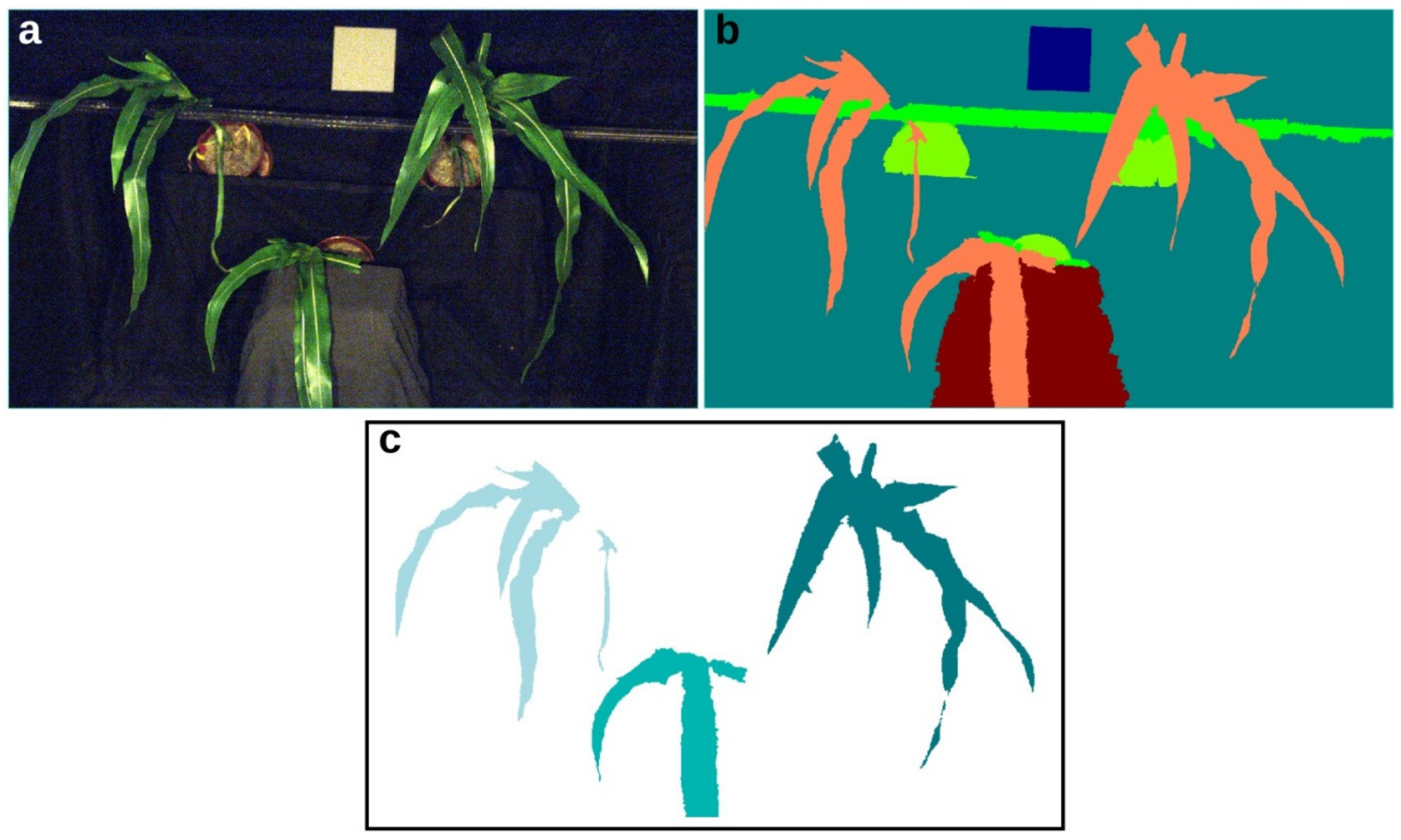
2.3.2. Hyperspectral Imaging
2.3.3. Plant Morphology and Herbivory Damage
2.4. Statistical Analysis
2.5. Hyperspectral Data Preprocessing and Analysis
3. Results
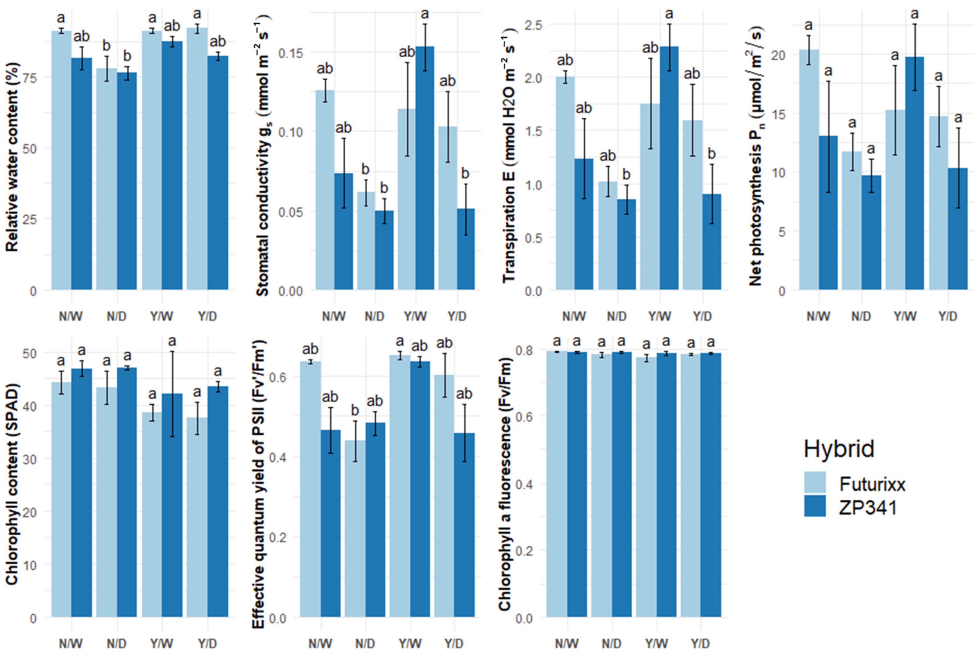
3.1. Physiological Parameters
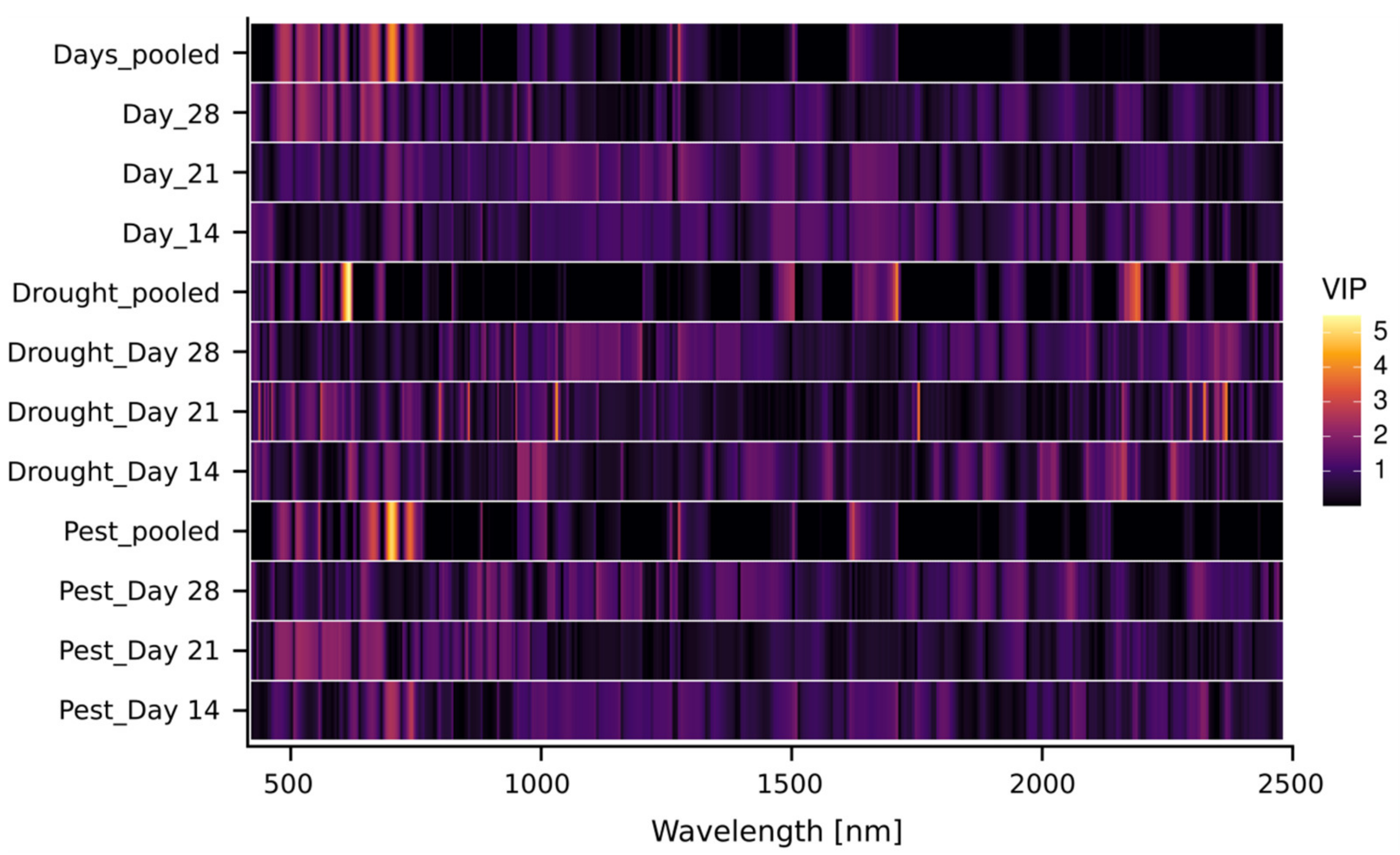
3.2. Hyperspectral Imaging
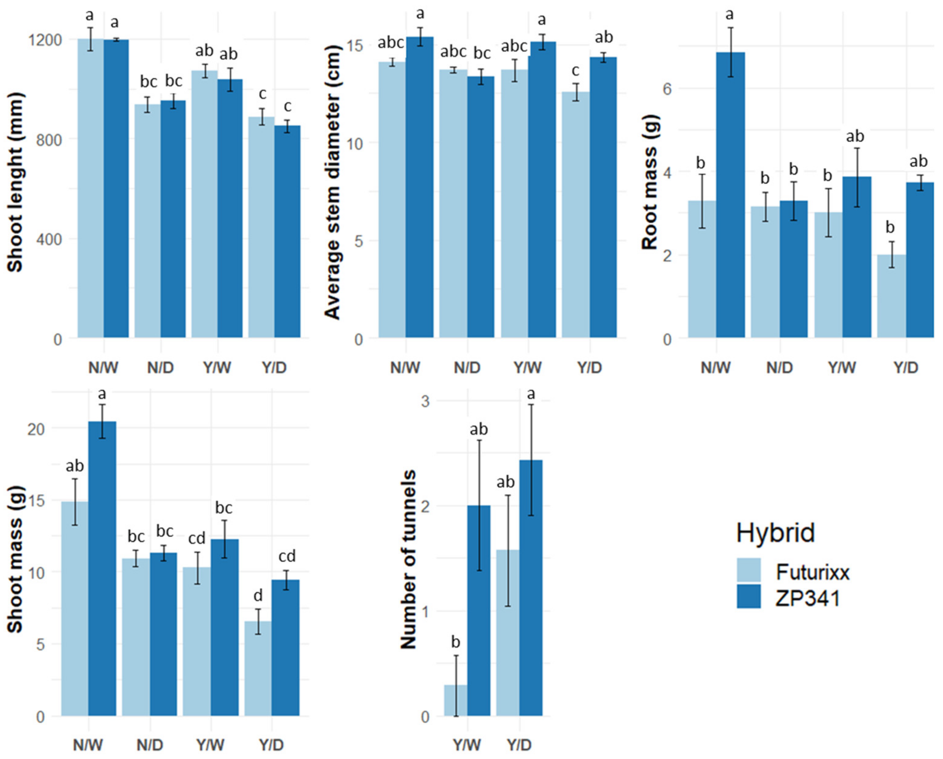
3.3. Plant Morphology
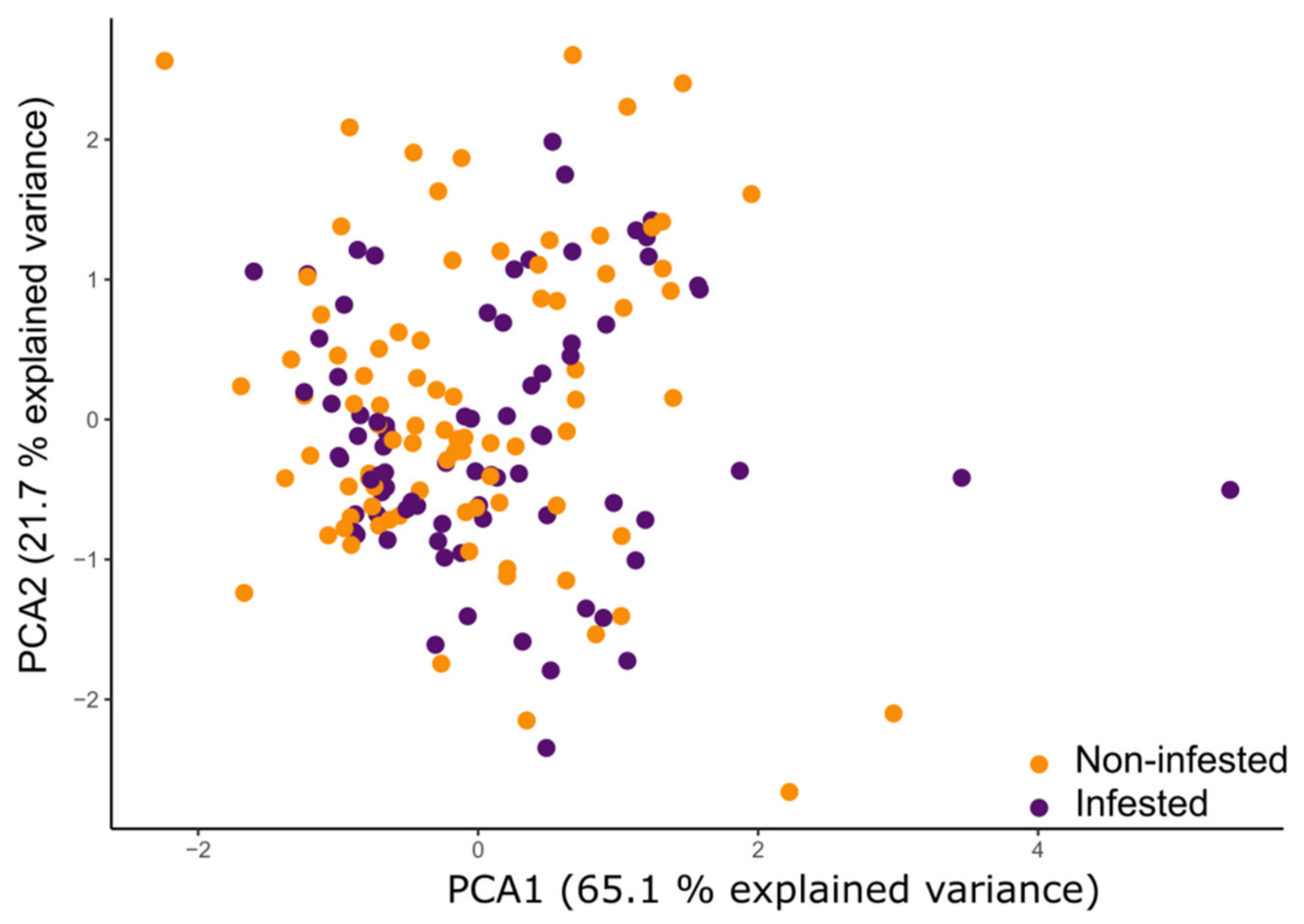
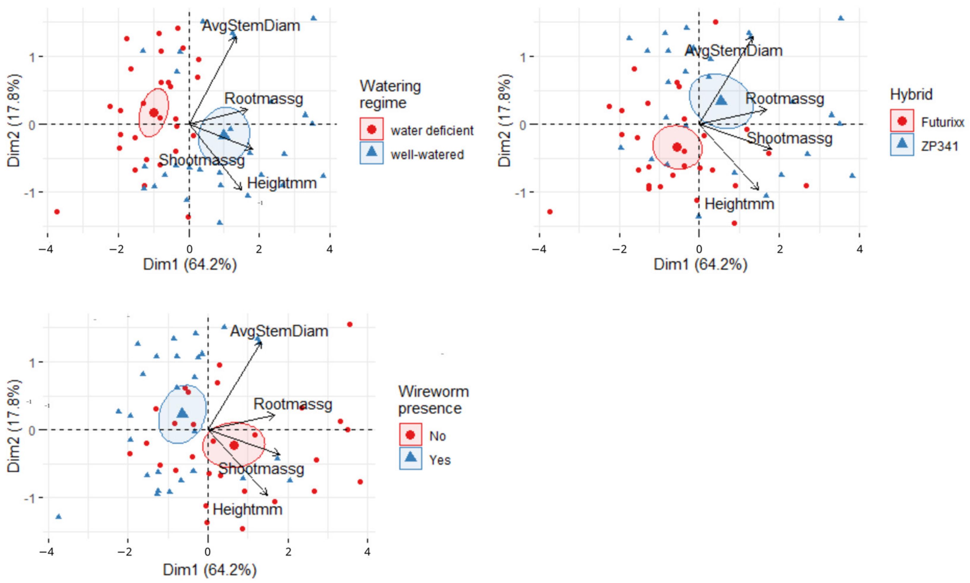
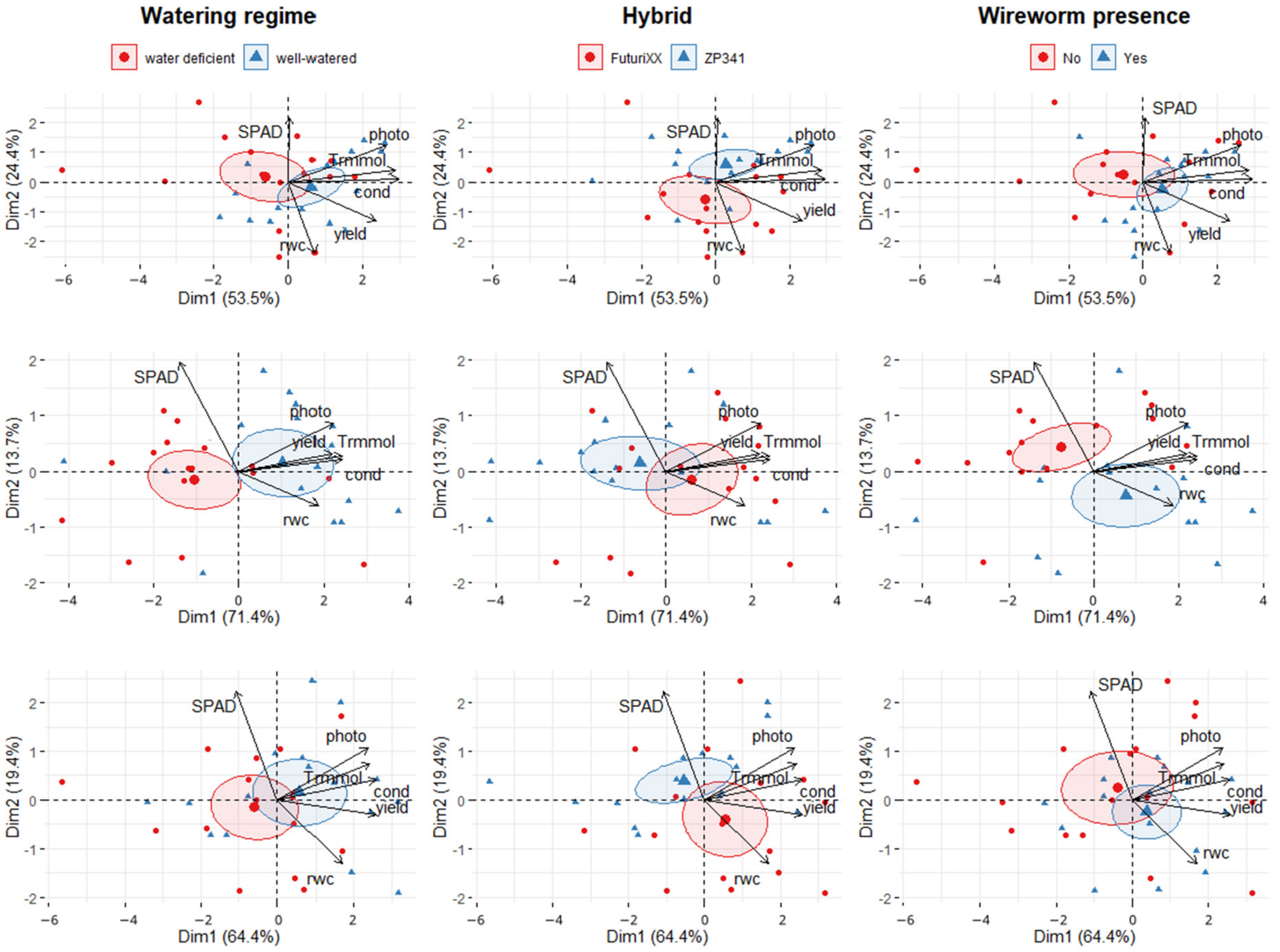
3.4. PCA of Physiological and Morphological Maize Parameters
3.5. Herbivory Damage
4. Discussion
5. Conclusions
Supplementary Materials
Author Contributions
Funding
Data Availability Statement
Acknowledgments
Conflicts of Interest
References
- Bento, V.A.; Ribeiro, A.F.S.; Russo, A.; Gouveia, C.M.; Cardoso, R.M.; Soares, P.M.M. The impact of climate change in wheat and barley yields in the Iberian Peninsula. Sci. Rep. 2021, 11, 15484. [Google Scholar] [CrossRef] [PubMed]
- Jennings, S.A.; Koehler, A.K.; Nicklin, K.J.; Deva, C.; Sait, S.M.; Challinor, A.J. Global Potato Yields Increase Under Climate Change with Adaptation and CO2 Fertilisation. Front. Sustain. Food Syst. 2020, 4. [Google Scholar] [CrossRef]
- Potopová, V.; Lhotka, O.; Možný, M.; Musiolková, M. Vulnerability of hop-yields due to compound drought and heat events over European key-hop regions. Int. J. Climatol. 2021, 41, E2136–E2158. [Google Scholar] [CrossRef]
- Jacobs, C.; Berglund, M.; Kurnik, B.; Dworak, T.; Marras, S.; Mereu, V.; Michetti, M. Climate Change Adaptation in the Agriculture Sector in Europe (4/2019); European Environment Agency: Copenhagen, Denmark, 2019. [Google Scholar]
- Chen, J.; Xu, W.; Velten, J.; Xin, Z.; Stout, J. Characterization of maize inbred lines for drought and heat tolerance. J. Soil Water Conserv. 2012, 67, 354–364. [Google Scholar] [CrossRef] [Green Version]
- Westgate, M.E.; Boyer, J.S. Osmotic adjustment and the inhibition of leaf, root, stem.pdf. Planta 1985, 164, 540–549. [Google Scholar] [CrossRef]
- Skendžić, S.; Zovko, M.; Živković, I.P.; Lešić, V.; Lemić, D. The Impact of Climate Change on Agricultural Insect Pests. Insects 2021, 12, 440. [Google Scholar] [CrossRef]
- Veres, A.; Wyckhuys, K.A.G.; Kiss, J.; Tóth, F.; Burgio, G.; Pons, X.; Avilla, C.; Vidal, S.; Razinger, J.; Bazok, R.; et al. An update of the Worldwide Integrated Assessment (WIA) on systemic pesticides. Part 4: Alternatives in major cropping systems. Environ. Sci. Pollut. Res. 2020, 27, 29867–29899. [Google Scholar] [CrossRef]
- Lohse, G.A. Familie: Elateridae. In Die Käfer Mitteleuropas, Bd. 6: Diversicornia (Lycidea-Byrrhidae); Freude, H., Ed.; Spektrum Akademischer Verlag: Heidelberg, Germany, 1979; pp. 103–186. [Google Scholar]
- Subklew, W. Agriotes lineatus L. und Agriotes obscurus L. (Ein Beitrag zu ihrer Morphologie und Biologie.). Zeitschrift für Angew. Entomol. 1934, 21, 96–122. [Google Scholar] [CrossRef]
- Furlan, L. The biology of Agriotes ustulatus Schaller (Col., Elateridae). II. Larval development, pupation, whole cycle description and practical implications. J. Appl. Entomol. 1998, 122, 71–78. [Google Scholar] [CrossRef]
- Furlan, L. The biology of Agriotes sordidus Illiger (Col., Elateridae). J. Appl. Entomol. 2004, 128, 696–706. [Google Scholar] [CrossRef]
- Saussure, S.; Plantegenest, M.; Thibord, J.B.; Larroudé, P.; Poggi, S. Management of wireworm damage in maize fields using new, landscape-scale strategies. Agron. Sustain. Dev. 2015, 35, 793–802. [Google Scholar] [CrossRef] [Green Version]
- Furlan, L.; Contiero, B.; Chiarini, F.; Colauzzi, M.; Sartori, E.; Benvegnù, I.; Fracasso, F.; Giandon, P. Risk assessment of maize damage by wireworms (Coleoptera: Elateridae) as the first step in implementing IPM and in reducing the environmental impact of soil insecticides. Environ. Sci. Pollut. Res. 2017, 24, 236–251. [Google Scholar] [CrossRef] [Green Version]
- Kozina, A.; Lemic, D.; Bazok, R.; Mikac, K.M.; Mclean, C.M.; Ivezić, M.; Igrc Barčić, J.; Aukema, B. Climatic, edaphic factors and cropping history help predict click beetle (Coleoptera: Elateridae) (Agriotes spp.) abundance. J. Insect Sci. 2015, 15, 1–8. [Google Scholar] [CrossRef]
- Staudacher, K.; Schallhart, N.; Pitterl, P.; Wallinger, C.; Brunner, N.; Landl, M.; Kromp, B.; Glauninger, J.; Traugott, M. Occurrence of Agriotes wireworms in Austrian agricultural land. J. Pest Sci. 2013, 86, 33–39. [Google Scholar] [CrossRef] [Green Version]
- Čamprag, D. Skočibube (Elateridae) i Integralne Mere Suzbijanja; Poljoprivredni Fakultet, Institut za Zaštitu Bilja, Design Studio Stanišić: Novi Sad, Serbia, 1997. [Google Scholar]
- Radcliffe, E.B.; Lagnaoui, A. Insect pests in potato. In Potato Biology and Biotechnology: Advances and Perspectives; Vreugdenhil, D., Ed.; Elsevier B.V.: Amsterdam, The Netherlands, 2007; pp. 543–567. ISBN 9780444510181. [Google Scholar]
- Jones, E.W. Laboratory Studies on the Moisture Relations of Limonius (Coleoptera: Elaterida). Ecology 1951, 32, 284–293. [Google Scholar] [CrossRef]
- Voigt, C.A. Callose-mediated resistance to pathogenic intruders in plant defense-related papillae. Front. Plant Sci. 2014, 5, 1–6. [Google Scholar] [CrossRef]
- Susič, N.; Žibrat, U.; Sinkovič, L.; Vončina, A.; Razinger, J.; Knapič, M.; Sedlar, A.; Širca, S.; Gerič Stare, B. From Genome to Field—Observation of the Multimodal Nematicidal and Plant Growth-Promoting Effects of Bacillus firmus I-1582 on Tomatoes Using Hyperspectral Remote Sensing. Plants 2020, 9, 592. [Google Scholar] [CrossRef]
- Brugger, A.; Behmann, J.; Paulus, S.; Luigs, H.-G.; Kuska, M.T.; Schramowski, P.; Kersting, K.; Steiner, U.; Mahlein, A.-K. Extending Hyperspectral Imaging for Plant Phenotyping to the UV-Range. Remote Sens. 2019, 11, 1401. [Google Scholar] [CrossRef] [Green Version]
- Abd El-Ghany, N.M.; Abd El-Aziz, S.E.; Marei, S.S. A review: Application of remote sensing as a promising strategy for insect pests and diseases management. Environ. Sci. Pollut. Res. 2020, 27, 33503–33515. [Google Scholar] [CrossRef]
- Wójtowicz, M.; Wójtowicz, A.; Piekarczyk, J. Application of remote sensing methods in agriculture. Commun. Biometry Crop Sci. 2016, 11, 31–50. [Google Scholar]
- Acker, J.; Williams, R.; Chiu, L.; Ardanuy, P.; Miller, S.; Schueler, C.; Vachon, P.W.; Manore, M. Remote Sensing from Satellites. In Reference Module in Earth Systems and Environmental Sciences; Elsevier: Amsterdam, The Netherlands, 2014. [Google Scholar]
- Terentev, A.; Dolzhenko, V.; Fedotov, A.; Eremenko, D. Current State of Hyperspectral Remote Sensing for Early Plant Disease Detection: A Review. Sensors 2022, 22, 757. [Google Scholar] [CrossRef] [PubMed]
- Susič, N.; Žibrat, U.; Širca, S.; Strajnar, P.; Razinger, J.; Knapič, M.; Vončina, A.; Urek, G.; Gerič Stare, B. Discrimination between abiotic and biotic drought stress in tomatoes using hyperspectral imaging. Sens. Actuators B Chem. 2018, 273, 842–852. [Google Scholar] [CrossRef] [Green Version]
- Santos, L.B.; Bastos, L.M.; de Oliveira, M.F.; Soares, P.L.M.; Ciampitti, I.A.; da Silva, R.P. Identifying Nematode Damage on Soybean through Remote Sensing and Machine Learning Techniques. Agronomy 2022, 12, 2404. [Google Scholar] [CrossRef]
- Hunt, E.R.; Rondon, S.I. Detection of potato beetle damage using remote sensing from small unmanned aircraft systems. J. Appl. Remote Sens. 2017, 11, 026013. [Google Scholar] [CrossRef] [Green Version]
- Yang, Z.; Rao, M.N.; Elliott, N.C.; Kindler, S.D.; Popham, T.W. Differentiating stress induced by greenbugs and Russian wheat aphids in wheat using remote sensing. Comput. Electron. Agric. 2009, 67, 64–70. [Google Scholar] [CrossRef]
- Iost Filho, F.H.; de Bastos Pazini, J.; de Medeiros, A.D.; Rosalen, D.L.; Yamamoto, P.T. Assessment of Injury by Four Major Pests in Soybean Plants Using Hyperspectral Proximal Imaging. Agronomy 2022, 12, 1516. [Google Scholar] [CrossRef]
- Zhang, X.; Liu, F.; He, Y.; Li, X. Application of hyperspectral imaging and chemometric calibrations for variety discrimination of maize seeds. Sensors 2012, 12, 17234–17246. [Google Scholar] [CrossRef]
- Williams, P.; Geladi, P.; Fox, G.; Manley, M. Maize kernel hardness classification by near infrared (NIR) hyperspectral imaging and multivariate data analysis. Anal. Chim. Acta 2009, 653, 121–130. [Google Scholar] [CrossRef]
- Oglesby, C.; Fox, A.A.A.; Singh, G.; Dhillon, J. Predicting In-Season Corn Grain Yield Using Optical Sensors. Agronomy 2022, 12, 2402. [Google Scholar] [CrossRef]
- Wang, S.; Guan, K.; Wang, Z.; Ainsworth, E.A.; Zheng, T.; Townsend, P.A.; Liu, N.; Nafziger, E.; Masters, M.D.; Li, K.; et al. Airborne hyperspectral imaging of nitrogen deficiency on crop traits and yield of maize by machine learning and radiative transfer modeling. Int. J. Appl. Earth Obs. Geoinf. 2021, 105, 102617. [Google Scholar] [CrossRef]
- Feng, X.; Zhao, Y.; Zhang, C.; Cheng, P.; He, Y. Discrimination of transgenic maize kernel using NIR hyperspectral imaging and multivariate data analysis. Sensors 2017, 17, 1894. [Google Scholar] [CrossRef]
- Dhau, I.; Adam, E.; Mutanga, O.; Ayisi, K.K. Detecting the severity of maize streak virus infestations in maize crop using in situ hyperspectral data. Trans. R. Soc. S. Afr. 2017, 73, 8–15. [Google Scholar] [CrossRef]
- Del Fiore, A.; Reverberi, M.; Ricelli, A.; Pinzari, F.; Serranti, S.; Fabbri, A.A.; Bonifazi, G.; Fanelli, C. Early detection of toxigenic fungi on maize by hyperspectral imaging analysis. Int. J. Food Microbiol. 2010, 144, 64–71. [Google Scholar] [CrossRef]
- Zhao, X.; Wang, W.; Chu, X.; Li, C.; Kimuli, D. Early detection of Aspergillus parasiticus infection in maize kernels using near-infrared hyperspectral imaging and multivariate data analysis. Appl. Sci. 2017, 7, 90. [Google Scholar] [CrossRef] [Green Version]
- Williams, P.J.; Geladi, P.; Britz, T.J.; Manley, M. Investigation of fungal development in maize kernels using NIR hyperspectral imaging and multivariate data analysis. J. Cereal Sci. 2012, 55, 272–278. [Google Scholar] [CrossRef]
- Ausmus, B.S.; Hilty, J.W. Reflectance studies of healthy, maize dwarf mosaic virus-infected, and Helminthosporium maydis-infected corn leaves. Remote Sens. Environ. 1971, 2, 77–81. [Google Scholar] [CrossRef]
- Garcia Furuya, D.E.; Ma, L.; Faita Pinheiro, M.M.; Georges Gomes, F.D.; Gonçalvez, W.N.; Junior, J.M.; de Castro Rodrigues, D.; Blassioli-Moraes, M.C.; Furtado Michereff, M.F.; Borges, M.; et al. Prediction of insect-herbivory-damage and insect-type attack in maize plants using hyperspectral data. Int. J. Appl. Earth Obs. Geoinf. 2021, 105, 102608. [Google Scholar] [CrossRef]
- Chávez-Arias, C.C.; Ligarreto-Moreno, G.A.; Ramírez-Godoy, A.; Restrepo-Díaz, H. Maize Responses Challenged by Drought, Elevated Daytime Temperature and Arthropod Herbivory Stresses: A Physiological, Biochemical and Molecular View. Front. Plant Sci. 2021, 12, 702841. [Google Scholar] [CrossRef]
- Kölliker, U.; Jossi, W.; Kuske, S. Optimised protocol for wireworm rearing. IOBC/WPRS Bull. 2009, 45, 457–460. [Google Scholar]
- van Herk, W.G.; Vernon, R.S. Categorization and numerical assessment of wireworm mobility over time following exposure to bifenthrin. J. Pest Sci. 2013, 86, 115–123. [Google Scholar] [CrossRef]
- Hartung, J.; Wagener, J.; Ruser, R.; Piepho, H.P. Blocking and re-arrangement of pots in greenhouse experiments: Which approach is more effective? Plant Methods 2019, 15, 143. [Google Scholar] [CrossRef] [PubMed] [Green Version]
- Lichtenthaler, H.K.; Buschmann, C.; Knapp, M. How to correctly determine the different chlorophyll fluorescence parameters and the chlorophyll fluorescence decrease ratio RFd of leaves with the PAM fluorometer. Photosynthetica 2005, 43, 379–393. [Google Scholar] [CrossRef]
- Kramer, P.J.; Boyer, J.S. Water Relations of Plants and Soils; Academic Press, Inc.: New York, NY, USA, 1995; ISBN 978-0124250604. [Google Scholar]
- Piqueras, S.; Burger, J.; Tauler, R.; de Juan, A. Relevant aspects of quantification and sample heterogeneity in hyperspectral image resolution. Chemom. Intell. Lab. Syst. 2012, 117, 169–182. [Google Scholar] [CrossRef]
- Park, E.; Cho, M.; Ki, C.S. Correct use of repeated measures analysis of variance. Korean J. Lab. Med. 2009, 29, 1–9. [Google Scholar] [CrossRef] [PubMed] [Green Version]
- Kassambara, A. rstatix: Pipe-Friendly Framework for Basic Statistical Tests. R Package Version 0.7.0 2021. Available online: https://rpkgs.datanovia.com/rstatix/ (accessed on 15 September 2021).
- Wickham, H.; Averick, M.; Bryan, J.; Chang, W.; McGowan, L.; François, R.; Grolemund, G.; Hayes, A.; Henry, L.; Hester, J.; et al. Welcome to the Tidyverse. J. Open Source Softw. 2019, 4, 1686. [Google Scholar] [CrossRef] [Green Version]
- Lenth, R.V. emmeans: Estimated Marginal Means, aka Least-Squares Means. R Package Version 1.7.1-1. 2021. Available online: https://CRAN.R-project.org/package=emmeans (accessed on 15 September 2021).
- R Core Team. R: A Language and Environment for Statistical Computing; R Foundation for Statistical Computing: Vienna, Austria, 2019; Available online: https://www.R-project.org/ (accessed on 1 March 2021).
- Le, S.; Josse, J.; Husson, F. FactoMineR: An R Package for Multivariate Analysis. J. Stat. Softw. 2008, 25. [Google Scholar] [CrossRef] [Green Version]
- Kassambara, A.; Mundt, F. factoextra: Extract and Visualize the Results of Multivariate Data Analyses. R Package Version 1.0.7. 2020. Available online: https://rpkgs.datanovia.com/factoextra/index.html (accessed on 16 September 2021).
- Anderson, M.J. A new method for non-parametric multivariate analysis of variance. Austral Ecol. 2001, 26, 32–46. [Google Scholar] [CrossRef]
- Salazar, G. EcolUtils: Utilities for Community Ecology Analysis. R Package Version 0.1. 2022. Available online: https://rdrr.io/github/GuillemSalazar/EcolUtils/man/EcolUtils.html (accessed on 22 September 2021).
- Oksanen, J.; Guillaume Blanchet, F.; Friendly, M.; Kindt, R.; Legendre, P.; McGlinn, D.; Minchin, P.R.; O’Hara, R.B.; Simpson, G.L.; Solymos, P.; et al. vegan: Community Ecology Package. R Package Version 2.5-7. 2020. Available online: https://CRAN.R-project.org/package=vegan (accessed on 17 September 2021).
- Chang, C.I. An information-theoretic approach to spectral variability, similarity, and discrimination for hyperspectral image analysis. IEEE Trans. Inf. Theory 2000, 46, 1927–1932. [Google Scholar] [CrossRef] [Green Version]
- Agricultural Institute of Slovenia. SiaPy: A Tool for Efficient Processing of Spectral Images with Python. Python Package v1.0.0. 2022. Available online: https://zenodo.org/record/7409194#.Y5sgP0nMIuU (accessed on 1 September 2022).
- Lê Cao, K.-A.; Boitard, S.; Besse, P. Sparse PLS discriminant analysis: Biologically relevant feature selection and graphical displays for multiclass problems. BMC Bioinform. 2011, 12, 253. [Google Scholar] [CrossRef] [Green Version]
- Rohart, F.; Gautier, B.; Singh, A.; Lê Cao, K.A. mixOmics: An R package for ‘omics feature selection and multiple data integration. PLoS Comput. Biol. 2017, 13, e1005752. [Google Scholar] [CrossRef] [Green Version]
- Karatzoglou, A.; Smola, A.; Hornik, K.; Zeileis, A. kernlab - An S4 Package for Kernel Methods in R. J. Stat. Softw. 2004, 11, 1–20. [Google Scholar] [CrossRef] [Green Version]
- Kuhn, M. Package ‘caret’: Classification and Regression Training 2021. Available online: https://CRAN.R-project.org/package=caret (accessed on 24 January 2022).
- Stevens, A.; Ramirez-Lopez, L. An Introduction to the Prospectr Package. R Package Vignette R Package Version 0.2.4.; R Foundation for Statistical Computing: Vienna, Austria, 2022. [Google Scholar]
- Wickham, H. ggplot2; Springer: New York, NY, USA, 2009; ISBN 978-0-387-98140-6. [Google Scholar]
- Microsoft, C.; Weston, S. doParallel: Foreach Parallel Adaptor for the “Parallel” Package. R Package Version 1.0.17. 2022. Available online: https://rdocumentation.org/packages/doParallel/versions/1.0.17 (accessed on 24 January 2022).
- Brereton, R.G.; Lloyd, G.R. Partial least squares discriminant analysis: Taking the magic away. J. Chemom. 2014, 28, 213–225. [Google Scholar] [CrossRef]
- Workman, J.; Weyer, L.J. Practical Guide and Spectral Atlas for Interpretative Near-Infrared Spectroscopy; CRC Press: New York, NY, USA, 2012; ISBN 9781439875254. [Google Scholar]
- Abd-Elgawad, M.M.M.; Kerlan, M.-C.; Molinari, S.; Abd-El-Kareem, F.; Kabeil, S.S.A.; Mohamad, M.M.; El-Nagdi, W.A. Histopathological Changes and Enzymatic Activities Induced by Meloidogyne incognita on Resistant and Susceptible Potato. Int. J. Phytopathol. 2012, 1, 62–72. [Google Scholar] [CrossRef]
- Anami, S.; De Block, M.; MacHuka, J.; Van Lijsebettens, M. Molecular improvement of tropical maize for drought stress tolerance in Sub-Saharan Africa. CRC. Crit. Rev. Plant Sci. 2009, 28, 16–35. [Google Scholar] [CrossRef]
- Çakir, R. Effect of water stress at different development stages on vegetative and reproductive growth of corn. F. Crop. Res. 2004, 89, 1–16. [Google Scholar] [CrossRef]
- Álvarez-Iglesias, L.; Roza-Delgado, B.D.L.; Reigosa, M.J.; Revilla, P.; Pedrol, N. A simple, fast and accurate screening method to estimate maize (Zea mays L.) tolerance to drought at early stages. Maydica 2017, 62, 34. [Google Scholar]
- Ye, J.; Wang, S.; Deng, X.; Yin, L.; Xiong, B.; Wang, X. Melatonin increased maize (Zea mays L.) seedling drought tolerance by alleviating drought-induced photosynthetic inhibition and oxidative damage. Acta Physiol. Plant. 2016, 38, 48. [Google Scholar] [CrossRef]
- Taupin, P. Panorama des Une lutte de longue haleine. Perspect. Agric. 2007, 339, 27–31. [Google Scholar]
- Staley, J.T.; Hodgson, C.J.; Mortimer, S.R.; Morecroft, M.D.; Masters, G.J.; Brown, V.K.; Taylor, M.E. Effects of summer rainfall manipulations on the abundance and vertical distribution of herbivorous soil macro-invertebrates. Eur. J. Soil Biol. 2007, 43, 189–198. [Google Scholar] [CrossRef]
- Furlan, L. The biology of Agriotes ustulatus Schäller (Col., Elateridae). I. Adults and oviposition. J. Appl. Entomol. 1996, 120, 269–274. [Google Scholar] [CrossRef]
- Miles, H.W. Wireworms and Agriculture, With Special Reference To Agriotes obscurus L. Ann. Appl. Biol. 1942, 29, 176–180. [Google Scholar] [CrossRef]
- Mattson, W.J.; Haack, R.A. The Role of Drought in Outbreaks of Plant-Eating Insects. Bioscience 1987, 37, 110–118. [Google Scholar] [CrossRef]
- Copolovici, L.; Kännaste, A.; Remmel, T.; Niinemets, Ü. Volatile organic compound emissions from Alnus glutinosa under interacting drought and herbivory stresses. Environ. Exp. Bot. 2014, 100, 55–63. [Google Scholar] [CrossRef] [PubMed] [Green Version]
- Nguyen, D.; D’Agostino, N.; Tytgat, T.O.G.; Sun, P.; Lortzing, T.; Visser, E.J.W.; Cristescu, S.M.; Steppuhn, A.; Mariani, C.; van Dam, N.M.; et al. Drought and flooding have distinct effects on herbivore-induced responses and resistance in Solanum dulcamara. Plant Cell Environ. 2016, 39, 1485–1499. [Google Scholar] [CrossRef] [PubMed]
- Bansal, S.; Hallsby, G.; Löfvenius, M.O.; Nilsson, M.C. Synergistic, additive and antagonistic impacts of drought and herbivory on Pinus sylvestris: Leaf, tissue and whole-plant responses and recovery. Tree Physiol. 2013, 33, 451–463. [Google Scholar] [CrossRef] [Green Version]
- Bauerfeind, S.S.; Fischer, K. Testing the plant stress hypothesis: Stressed plants offer better food to an insect herbivore. Entomol. Exp. Appl. 2013, 149, 148–158. [Google Scholar] [CrossRef]
- Rosa, E.; Minard, G.; Lindholm, J.; Saastamoinen, M. Moderate plant water stress improves larval development, and impacts immunity and gut microbiota of a specialist herbivore. PLoS ONE 2019, 14, e0204292. [Google Scholar] [CrossRef]
- Furlan, L.; Kreutzweiser, D. Alternatives to neonicotinoid insecticides for pest control: Case studies in agriculture and forestry. Environ. Sci. Pollut. Res. 2015, 22, 135–147. [Google Scholar] [CrossRef] [Green Version]
- Traugott, M.; Benefer, C.M.; Blackshaw, R.P.; van Herk, W.G.; Vernon, R.S. Biology, Ecology, and Control of Elaterid Beetles in Agricultural Land. Annu. Rev. Entomol. 2015, 60, 313–334. [Google Scholar] [CrossRef] [Green Version]
- Furlan, L.; Contiero, B.; Chiarini, F.; Benvegnù, I.; Tóth, M. The use of click beetle pheromone traps to optimize the risk assessment of wireworm (Coleoptera: Elateridae) maize damage. Sci. Rep. 2020, 10, 8780. [Google Scholar] [CrossRef]


| Treatment | Hybrid | Pest | Watering Regime |
|---|---|---|---|
| N/D | ZP341 | No | D |
| N/W | ZP341 | No | W |
| N/D | FuturiXX | No | D |
| N/W | FuturiXX | No | W |
| Y/D | ZP341 | Yes | D |
| Y/W | ZP341 | Yes | W |
| Y/D | FuturiXX | Yes | D |
| Y/W | FuturiXX | Yes | W |
| Date | DPES a | DPSI b | BBCH c | Activity |
|---|---|---|---|---|
| 9 April 2020 | 0 | 0 | 0 | Planting the maize |
| 6 May 2020 | 27 | 0 | 34 | Adding wireworms and changing watering regime |
| 20 May 2020 | 41 | 14 | 35 | Acquisition of physiological parameters and hyperspectral imaging |
| 27 May 2020 | 48 | 21 | 35 | Acquisition of physiological parameters and hyperspectral imaging |
| 3 June 2020 | 55 | 28 | 35 | Acquisition of physiological parameters and hyperspectral imaging |
| 4 June 2020 | 56 | 29 | 35 | Acquisition of morphological parameters and termination of the experiment |
| Hybrid | Treatment | Rwc (%) a | gs (mmol m−2 s−1) b | E (mmol H2O m−2 s−1) c | PN (µmol/m2/s) d | SPAD e | Fv’/Fm’ f | Fv/Fm g | |
|---|---|---|---|---|---|---|---|---|---|
| DAY 14 | ZP341 | N/D | 92.68 ± 1.49 a | 0.11 ± 0.02 a | 1.35 ± 0.20 a | 18.74 ± 2.75 a | 49.08 ± 1.55 a | 0.58 ± 0.02 a | 0.79 ± 0.00 a |
| N/W | 96.06 ± 0.50 a | 0.16 ± 0.02 a | 2.04 ± 0.25 a | 26.50 ± 1.99 a | 49.13 ± 1.18 a | 0.58 ± 0.02 a | 0.78 ± 0.00 ab | ||
| Y/D | 91.77 ± 2.88 a | 0.13 ± 0.02 a | 1.76 ± 0.12 a | 23.81 ± 2.09 a | 46.93 ± 0.95 a | 0.58 ± 0.02 a | 0.76 ± 0.01 abc | ||
| Y/W | 96.34 ± 1.35 a | 0.15 ± 0.01 a | 1.99 ± 0.29 a | 23.79 ± 3.99 a | 44.30 ± 2.47 a | 0.61 ± 0.01 a | 0.78 ± 0.01 ab | ||
| FuturiXX | N/D | 96.36 ± 10.31 a | 0.09 ± 0.03 a | 1.22 ± 0.27 a | 15.37 ± 4.53 a | 46.70 ± 2.86 a | 0.50 ± 0.07 a | 0.78 ± 0.00 ab | |
| N/W | 97.73 ± 0.59 a | 0.13 ± 0.02 a | 1.71 ± 0.30 a | 19.73 ± 2.40 a | 41.33 ± 2.00 a | 0.60 ± 0.02 a | 0.77 ± 0.01 abc | ||
| Y/D | 102.65 ± 3.69 a | 0.14 ± 0.01 a | 1.90 ± 0.23 a | 19.60 ± 2.39 a | 43.70 ± 1.78 a | 0.63 ± 0.01 a | 0.75 ± 0.01 bc | ||
| Y/W | 101.67 ± 4.31 a | 0.14 ± 0.01 a | 1.96 ± 0.25 a | 20.37 ± 2.02 a | 42.98 ± 1.46 a | 0.61 ± 0.02 a | 0.74 ± 0.01 c | ||
| DAY 21 | ZP341 | N/D | 76.23 ± 2.22 b | 0.05 ± 0.01 b | 0.85 ± 0.14 b | 9.70 ± 1.41 a | 47.08 ± 0.39 a | 0.48 ± 0.03 ab | 0.79 ± 0.00 a |
| N/W | 81.68 ± 4.01 ab | 0.07 ± 0.02 ab | 1.23 ± 0.38 ab | 13.02 ± 4.71 a | 46.88 ± 1.53 a | 0.47 ± 0.06 ab | 0.79 ± 0.00 a | ||
| Y/D | 82.30 ± 1.37 ab | 0.05 ± 0.02 b | 0.90 ± 0.28 b | 10.34 ± 3.40 a | 43.45 ± 1.05 a | 0.46 ± 0.07 ab | 0.79 ± 0.01 a | ||
| Y/W | 87.35 ± 1.79 ab | 0.15 ± 0.02 a | 2.28 ± 0.22 a | 19.74 ± 2.86 a | 37.73 ± 6.41 a | 0.64 ± 0.01 ab | 0.79 ± 0.01 a | ||
| FuturiXX | N/D | 77.97 ± 4.36 b | 0.06 ± 0.01 b | 1.02 ± 0.14 ab | 11.73 ± 1.58 a | 43.28 ± 3.20 a | 0.44 ± 0.05 b | 0.79 ± 0.00 a | |
| N/W | 91.08 ± 0.92 a | 0.13 ± 0.01 ab | 2.00 ± 0.06 ab | 20.39 ± 1.23 a | 44.23 ± 2.22 a | 0.63 ± 0.01 ab | 0.79 ± 0.00 a | ||
| Y/D | 92.07 ± 1.68 a | 0.10 ± 0.02 ab | 1.59 ± 0.34 ab | 14.71 ± 2.59 a | 37.50 ± 3.02 a | 0.60 ± 0.05 ab | 0.78 ± 0.00 a | ||
| Y/W | 91.22 ± 0.98 a | 0.11 ± 0.03 ab | 1.75 ± 0.43 ab | 15.24 ± 3.84 a | 38.63 ± 1.53 a | 0.65 ± 0.01 a | 0.78 ± 0.01 a | ||
| DAY 28 | ZP341 | N/D | 83.11 ± 5.88 a | 0.08 ± 0.03 a | 1.12 ± 0.39 a | 15.85 ± 5.40 a | 46.70 ± 1.00 a | 0.47 ± 0.08 a | 0.79 ± 0.00 a |
| N/W | 83.72 ± 4.29 a | 0.08 ± 0.03 a | 1.22 ± 0.38 a | 16.13 ± 4.13 a | 47.03 ± 1.56 a | 0.47 ± 0.05 a | 0.78 ± 0.00 a | ||
| Y/D | 85.08 ± 3.19 a | 0.08 ± 0.01 a | 1.39 ± 0.23 a | 15.40 ± 1.44 a | 44.00 ± 1.74 a | 0.49 ± 0.04 a | 0.79 ± 0.00 a | ||
| Y/W | 89.94 ± 2.32 a | 0.10 ± 0.02 a | 1.84 ± 0.38 a | 17.71 ± 2.88 a | 45.58 ± 1.82 a | 0.53 ± 0.05 a | 0.78 ± 0.01 a | ||
| FuturiXX | N/D | 83.96 ± 3.64 a | 0.07 ± 0.01 a | 1.17 ± 0.29 a | 14.40 ± 3.30 a | 44.28 ± 2.19 a | 0.47 ± 0.05 a | 0.79 ± 0.00 a | |
| N/W | 89.47 ± 3.61 a | 0.13 ± 0.03 a | 2.26 ± 0.47 a | 19.20 ± 2.53 a | 41.33 ± 3.68 a | 0.56 ± 0.05 a | 0.79 ± 0.01 a | ||
| Y/D | 91.09 ± 1.99 a | 0.09 ± 0.01 a | 1.49 ± 0.13 a | 16.23 ± 1.87 a | 38.03 ± 2.01 a | 0.56 ± 0.04 a | 0.78 ± 0.00 a | ||
| Y/W | 90.76 ± 1.66 a | 0.11 ± 0.01 a | 2.04 ± 0.38 a | 20.04 ± 1.59 a | 41.88 ± 2.09 a | 0.58 ± 0.04 a | 0.78 ± 0.00 a |
| Group a | N b | LV c | Var (%) d | Mahalanobis e | c f | Sigma g | OA h | Kappa i | Class j | Accuracy k | Sensitivity | Specificity | PPV l | NPV m | |
|---|---|---|---|---|---|---|---|---|---|---|---|---|---|---|---|
| Imaging session | 49 | 19 | 95.30 | 0.0176 | 10 | 0.011187 | 1 | 1 | 14 | 1 | 1 | 1 | 1 | 1 | |
| 21 | 1 | 1 | 1 | 1 | 1 | ||||||||||
| 28 | 1 | 1 | 1 | 1 | 1 | ||||||||||
| Treatment | 46 | 29 | 97.90 | 0.699 | 10 | 0.001 | 0.63 | 0.577 | ZP341 | N/D | 0.808 | 0.667 | 0.95 | 0.667 | 0.95 |
| N/W | 0.917 | 0.83 | 1 | 1 | 0.976 | ||||||||||
| Y/D | 0.975 | 1 | 0.95 | 0.75 | 1 | ||||||||||
| Y/W | 0.66 | 0.4 | 0.927 | 0.4 | 0.927 | ||||||||||
| FuturiXX | N/D | 0.78 | 0.667 | 0.9 | 0.5 | 0.947 | |||||||||
| N/W | 0.76 | 0.6 | 0.927 | 0.5 | 0.95 | ||||||||||
| Y/D | 0.58 | 0.167 | 1 | 1 | 0.889 | ||||||||||
| Y/W | 0.796 | 0.667 | 0.925 | 0.57 | 0.949 | ||||||||||
| Pest | 49 | 19 | 95.30 | 0.248 | 10 | 0.001 | 0.98 | 0.959 | / | 0.979 | 1 | 0.958 | 0.96 | 1 | |
| Drought | 49 | 13 | 90.50 | 0.379 | 10 | 0.001 | 0.959 | 0.918 | / | 0.96 | 0.92 | 1 | 1 | 0.92 |
| Group a | N b | LV c | Var (%) d | Mahalanobis e | c f | Sigma g | OA h | Kappa i | Class j | Accuracy k | Sensitivity | Specificity | PPV l | NPV m | |
|---|---|---|---|---|---|---|---|---|---|---|---|---|---|---|---|
| DAY 14 | 16 | 19 | 97.90 | 0.689 | 10 | 0.01018 | 0.867 | 0.847 | ZP341 | N/D | 0.808 | 0.667 | 0.95 | 0.667 | 0.95 |
| N/W | 0.917 | 0.83 | 1 | 1 | 0.976 | ||||||||||
| Y/D | 0.975 | 1 | 0.95 | 0.75 | 1 | ||||||||||
| Y/W | 0.66 | 0.4 | 0.927 | 0.4 | 0.927 | ||||||||||
| FuturiXX | N/D | 0.78 | 0.667 | 0.9 | 0.5 | 0.947 | |||||||||
| N/W | 0.76 | 0.6 | 0.927 | 0.5 | 0.95 | ||||||||||
| Y/D | 0.58 | 0.167 | 1 | 1 | 0.889 | ||||||||||
| Y/W | 0.796 | 0.667 | 0.925 | 0.57 | 0.949 | ||||||||||
| DAY 21 | 12 | 11 | 92.40 | 0.655 | 10 | 0.009059 | 0.833 | 0.81 | ZP341 | N/D | 0.7 | 0.5 | 0.9 | 0.5 | 0.9 |
| N/W | 0.7 | 0.5 | 0.9 | 0.5 | 0.9 | ||||||||||
| Y/D | 1 | 1 | 1 | 1 | 1 | ||||||||||
| Y/W | 1 | 1 | 1 | 1 | 1 | ||||||||||
| FuturiXX | N/D | 1 | 1 | 1 | 1 | 1 | |||||||||
| N/W | 1 | 1 | 1 | 1 | 1 | ||||||||||
| Y/D | 1 | 1 | 1 | 1 | 1 | ||||||||||
| Y/W | 1 | 1 | 1 | 1 | 1 | ||||||||||
| DAY 28 | 15 | 8 | 91.40 | 0.841 | 10 | 0.01 | 0.67 | 0.61 | ZP341 | N/D | 0.5 | 0 | 1 | 0 | 0.867 |
| N/W | 1 | 1 | 1 | 1 | 1 | ||||||||||
| Y/D | 0.67 | 0.5 | 0.846 | 0.333 | 0.92 | ||||||||||
| Y/W | 0.92 | 1 | 0.846 | 0.5 | 1 | ||||||||||
| FuturiXX | N/D | 0.96 | 1 | 0.92 | 0.67 | 1 | |||||||||
| N/W | 0.5 | 0 | 1 | 0 | 0.93 | ||||||||||
| Y/D | 0.75 | 0.5 | 1 | 1 | 0.93 | ||||||||||
| Y/W | 1 | 1 | 1 | 1 | 1 | ||||||||||
| pest_14 | 16 | 7 | 86.50 | 0.254 | 1000 | 0.0001 | 1 | 1 | 1 | 1 | 1 | 1 | 1 | ||
| pest_21 | 15 | 6 | 82 | 0.402 | 100 | 0.001 | 1 | 1 | 1 | 1 | 1 | 1 | 1 | ||
| pest_28 | 16 | 17 | 93.80 | 0.374 | 1000 | 0.0001 | 1 | 1 | 1 | 1 | 1 | 1 | 1 | ||
| drought _14 | 16 | 9 | 90.70 | 0.468 | 1000 | 0.0001 | 1 | 1 | 1 | 1 | 1 | 1 | 1 | ||
| drought _21 | 15 | 16 | 94.80 | 0.448 | 100 | 0.001 | 1 | 1 | 1 | 1 | 1 | 1 | 1 | ||
| drought _28 | 17 | 9 | 85 | 0.462 | 1000 | 0.0001 | 1 | 1 | 1 | 1 | 1 | 1 | 1 |
Disclaimer/Publisher’s Note: The statements, opinions and data contained in all publications are solely those of the individual author(s) and contributor(s) and not of MDPI and/or the editor(s). MDPI and/or the editor(s) disclaim responsibility for any injury to people or property resulting from any ideas, methods, instructions or products referred to in the content. |
© 2023 by the authors. Licensee MDPI, Basel, Switzerland. This article is an open access article distributed under the terms and conditions of the Creative Commons Attribution (CC BY) license (https://creativecommons.org/licenses/by/4.0/).
Share and Cite
Praprotnik, E.; Vončina, A.; Žigon, P.; Knapič, M.; Susič, N.; Širca, S.; Vodnik, D.; Lenarčič, D.; Lapajne, J.; Žibrat, U.; et al. Early Detection of Wireworm (Coleoptera: Elateridae) Infestation and Drought Stress in Maize Using Hyperspectral Imaging. Agronomy 2023, 13, 178. https://doi.org/10.3390/agronomy13010178
Praprotnik E, Vončina A, Žigon P, Knapič M, Susič N, Širca S, Vodnik D, Lenarčič D, Lapajne J, Žibrat U, et al. Early Detection of Wireworm (Coleoptera: Elateridae) Infestation and Drought Stress in Maize Using Hyperspectral Imaging. Agronomy. 2023; 13(1):178. https://doi.org/10.3390/agronomy13010178
Chicago/Turabian StylePraprotnik, Eva, Andrej Vončina, Primož Žigon, Matej Knapič, Nik Susič, Saša Širca, Dominik Vodnik, David Lenarčič, Janez Lapajne, Uroš Žibrat, and et al. 2023. "Early Detection of Wireworm (Coleoptera: Elateridae) Infestation and Drought Stress in Maize Using Hyperspectral Imaging" Agronomy 13, no. 1: 178. https://doi.org/10.3390/agronomy13010178