A Novel Regional-Scale Assessment of Soil Metal Pollution in Arid Agroecosystems

Abstract

This work is a novel trial to integrate geostatistics with fuzzy logic under the geographic information system (GIS) environment to model soil pollution. Soil samples from seventy-one soil profiles in the northern Nile Delta, Egypt, and were analyzed for total concentrations of Cd, Co, Cu, Pb, Ni, and Zn. Metal distribution maps were generated using ordinary kriging methods. They were normalized by linear and non-linear fuzzy membership functions (FMFs) and overlain by fuzzy operators (And, OR, Sum, Product, and Gamma). The final maps were validated using the area under the curve (AUC) of the receiver operating characteristic (ROC). The best-fitted semivariogram models were Gaussian for Cd, Pb, and Ni, circular for Co and Zn, and exponential for Cu. The ROC and AUC analysis revealed that the non-linear FMFs were more effective than the linear functions for modeling soil pollution. Overall, the highest AUC value (0.866; very good accuracy) resulted from applying the fuzzy Sum overly to the non-linearly normalized layers, implying the superiority of this model for decision-making in the studied area. Accordingly, 92% of the investigated soils were severely polluted. Our study would increase insight into soil metal pollution on a regional scale, especially in arid regions.

1. Introduction

Soil is a non-renewable resource that supports life on Earth by providing about 95% of global food production and offering other services like biomass production, securing natural resources, and maintaining biodiversity [1]. Yet, rapid urbanization and intensive industrial and agricultural activities accelerate degradation processes that diminish soil functions and ecosystem services [2]. Soil pollution is a chemical deterioration linked to the spread, accumulation, and negative biological or toxic effects of a substance on soils [3]. Potentially toxic metals (PTMs) are serious pollutants due to their fatal effects, bioaccumulation, and non-biodegradability [4]. Metals: Cu, Zu, and Ni play crucial roles in regulating the activity of several enzymes [5], while Co sustains the symbiotic N₂ fixation and manufacture of ethylene in legumes [6]. Other metals (Cd, Cr, and Pb) do not have positive roles and are highly toxic [7].

Excess of PTMs causes abiotic stress for soil biota via inhibiting enzyme activities, competition with essential cations, and generating oxidative stress [7]. Thus, the plant life cycle from seed germination to maturity stage is adversely affected, leading finally to reducing crop yield and quality [8]. However, numerous food, feed, and forage crops, known as hyperaccumulators, have a strong resistance to metal stress and can uptake excess PTMs and translocate them in their aerial parts [5,9]. Therefore, metals accumulated in soils can be enriched in animals and human organs through the food chain, leading to severe health risks [10]. The PTMs may also percolate into groundwater aquifers and deteriorate the groundwater quality [11,12]. Hence, a precise assessment of soil pollution based on PTMs is crucial to develop a proper remediation strategy and alleviate negative impacts [13].

The initial procedure for improved assessment of soil pollution is analyzing the spatial distribution of PTM content [14]. This analysis highlights hotspots of polluted areas and provides a key step in risk control [15]. Hence, the geographic information system (GIS) has been employed to map the spatial variability of PTMs in many soils around the world [16,17,18]. Geostatistical methods have been applied, including empirical Bayesian kriging in California, USA [19] and China [20], and kriging/cokriging in the UK [21] and Ireland [22]. Geostatistics provides a powerful tool to represent the spatial heterogeneity of soil attributes [22]. Therefore, it is frequently applied to estimate PTM concentrations at unsampled points from scattered measurements [20,21,22].

Kriging is a powerful geostatistical technique to analyze the spatial distribution of soil attributes and integrate data into raster maps through spatial interpolation [21,23,24]. Basically, it revolves around variograms and related parameters (nugget, sill, and range) to figure the spatial structure of soil variables [21,23]. Ordinary kriging (OK) is a basal application of this technique and provides an optimal and unbiased prediction [22]. OK simulates spatial variability via diverse variograms that can minimize the variance of prediction errors and offer various map outputs [25]. OK models have been applied to map PTMs in northern Tunisia [26], the Loess Plateau, China [27], south-central Turkey [28], and Upper Egypt [14]. Hence, modeling soil metal pollution using ordinary kriging maps is a promising approach.

Recently, mathematics-based models have been adopted to assess soil metal pollution. Herein, risk degrees are derived from the extent of deviation from reference values [4,13]. The uncertainty of this approach has been a big debate owing to the inconsistency of toxicity, various reference and ranking criteria, and subjectivity of simple and supervised classifications [13,29]. The GIS-fuzzy logic can handle these issues to develop more accurate classifiers and limits between categories [24]. Instead of the absolute membership in classical methods, the fuzzy membership functions (FMFs) precisely define the sensitivity of each pixel with a gradual scale from zero (no membership) to one (full membership). This decreases the vagueness and eliminates the error of uneven spacing of attributes [30,31]. The fuzzy overlay operators integrate normalized maps in diverging ways, offering more flexible combinations [32,33]. Hence, spatial models based on GIS-fuzzy logic improve insight into objective and precise monitoring of metal severity and associated risks.

In this context, GIS-fuzzy models have been adopted in previous works for marine sediment quality in China [34], surface water deterioration in Iran [30], and groundwater suitability in Bangladesh [35]. Unfortunately, such a robust approach has seldom been implemented in soil pollution studies, advocating an urgent need to test its performance in soil ecosystems. Thus, the present work is a trial toward a novel assessment of soil pollution by integrating geostatistics with fuzzy logic in the GIS platform. This relies mainly on (1) generating kriged maps for Cd, Co, Cu, Pb, Ni, and Zn, (2) normalizing these layers using FMFs, and (3) applying fuzzy overlay operators to generate overall pollution maps. The procedures are then applied in an area (the north Nile Delta, Egypt, in this case) typical for arid agro-ecosystems for the upcoming evaluations and environment protection in similar regions.

2. Materials and Methods

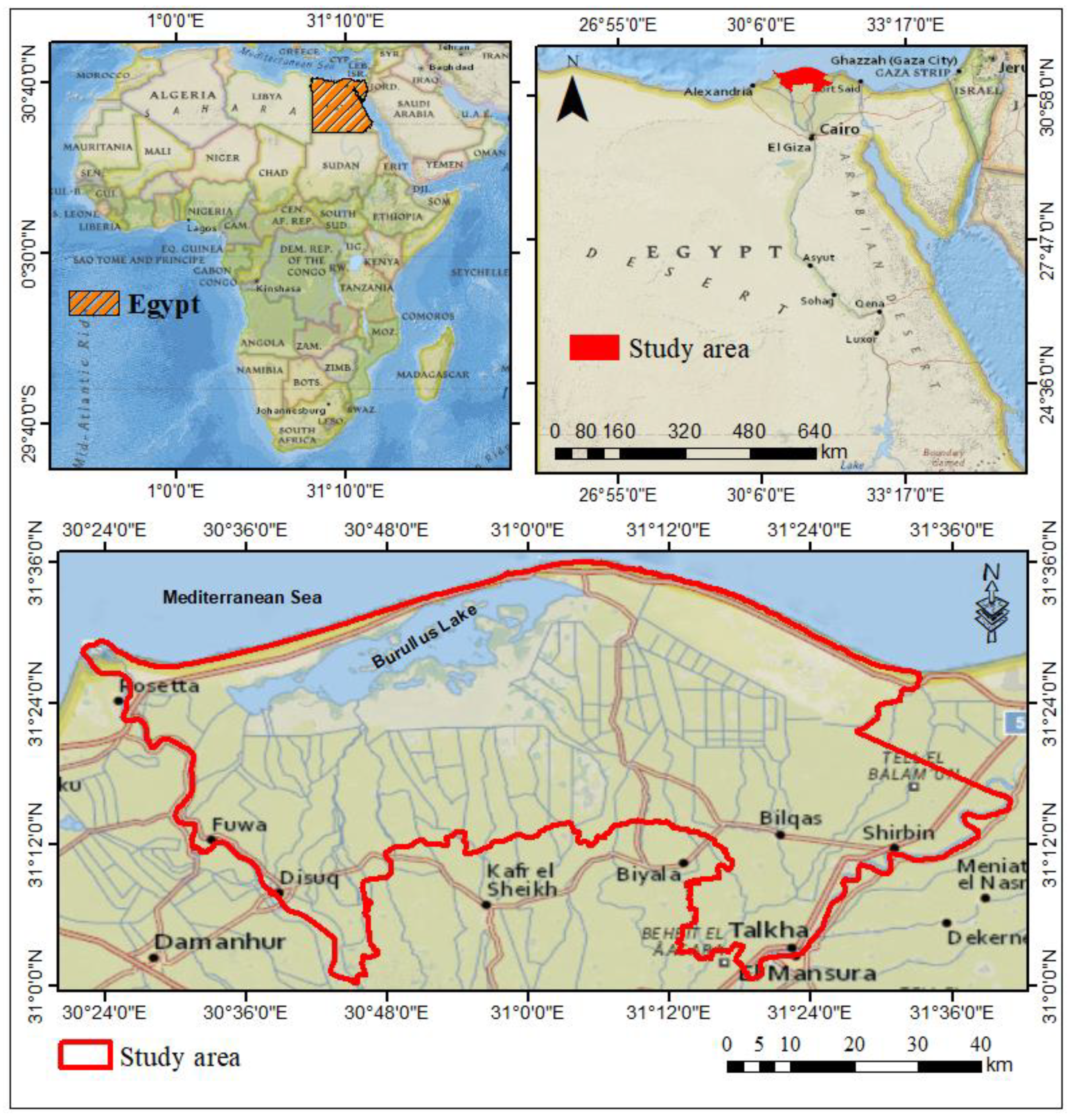
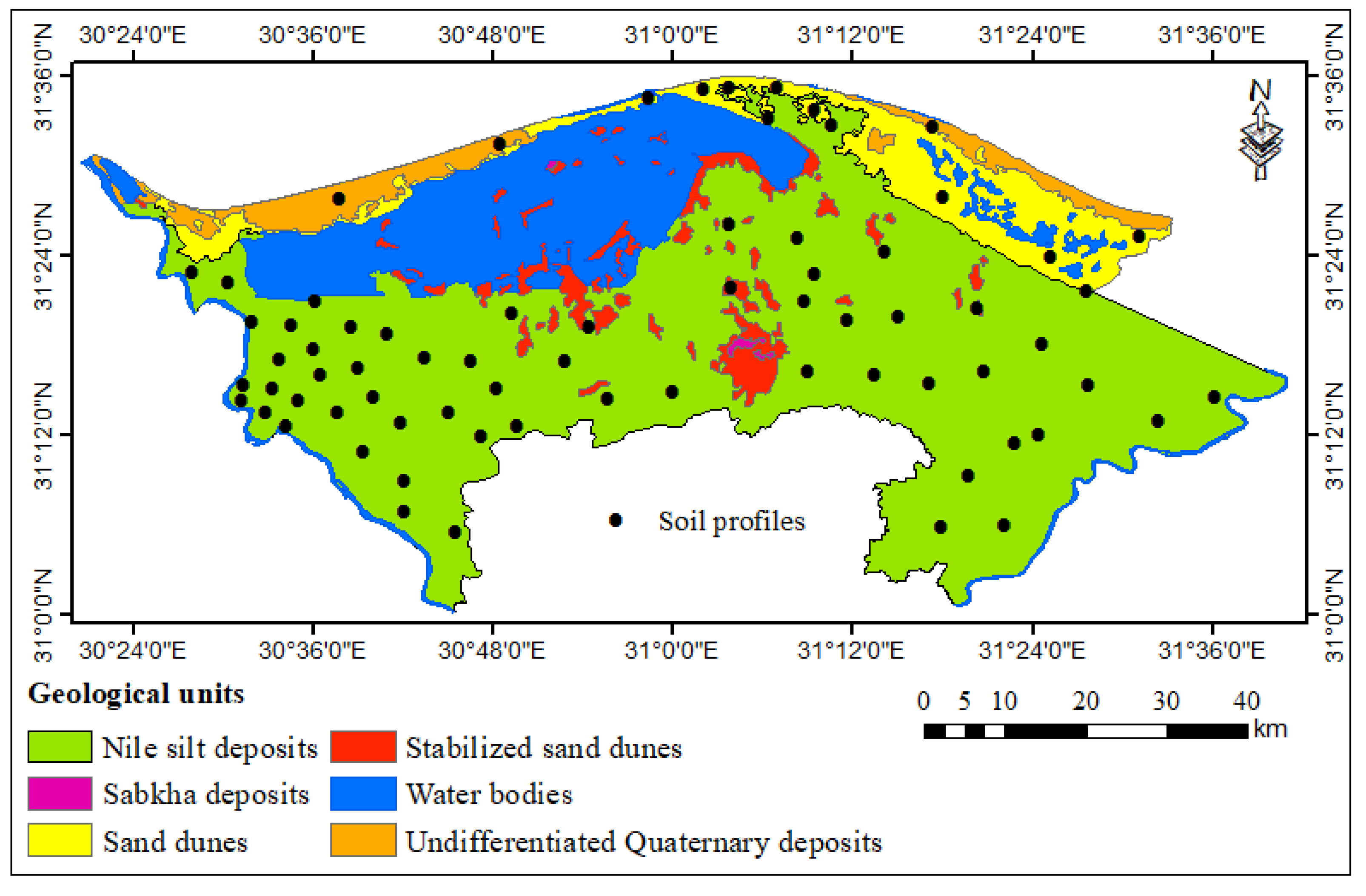
2.1. Study Area

The studied area lies in the northern Nile Delta of Egypt and covers 4319.26 km² in UTM zone 36 (latitude: 30°59′39.864″ to 31°36′33.116″ N; longitude: 30°20′23.622″ to 31°41′25.043″ E) (Figure 1). The elevation height ranges from 0 to 163 m above sea level and the slope gradient varies from 0 to 66%. The study area considerably supports food security as it includes a total cultivated area of 285,207 ha, providing major contributions to domestic production of food crops, i.e., rice, maize, and wheat. The area also provides a great portion of total fish production, where catch fisheries (marine, brackish, and freshwater) and aquaculture industries are mainly concentrated. The area is a heavily populated region, housing nearly 10 million inhabitants.

The climate is dominated by Mediterranean conditions with hot and arid summer and mild rains in winter. The mean annual temperature ranges from 14 to 25 °C, implying that the soil temperature regime varies from “thermic” to “hyperthermic” and the soil moisture regime is “torric” [36]. The total annual rainfall (R) varies from 56 to 227 mm, most of which occurs during the winter season. The potential evapotranspiration (PET) ranges between 2.9 and 5.5 mm per year. Hence, the aridity index (R/PET) varies from 0.05 to 0.16, indicating an arid climate as suggested by Prăvălie et al. [37].

The geological map of Egypt [38] reveals that the area is covered by sedimentary sequences of the Quaternary era (Figure 2). The Nile silt deposits (late Pleistocene-Holocene) dominate the majority of the area (67.95%). The Holocene deposits cover 13.33% of the total area and involve sand dunes (8.58%), stabilized sand dunes (4.61%), and sabkha (0.14%). Undifferentiated Quaternary formations dominate 4.26% of the total area, while water bodies occupy the remaining 18.12%.

The land use/land cover map (Figure S1) reveals four classes, i.e., water bodies, vegetation, urban areas, and barren land. The vegetation includes both natural halophytes (herbaceous plants and shrubs) in and around Burullus Lake, and crop lands, which cover the major area. The crop pattern is dominated by annual crops, covering nearly 99% of the cultivated lands [39]. Field crops occupy the major portion, where wheat and clover are the dominant winter crops, while rice and maize are commonly cultivated during the summer. Small areas are also cultivated by vegetable crops and fruit trees.

2.2. Field Work and Laboratory Analysis

Seventy-one geo-referenced soil profiles were randomly distributed across the area (manually) to represent different geological formations (Figure 2). The soil profiles were dug to a 150 cm depth or to permanent groundwater tables and the general features of each profile were delineated based on the Food and Agriculture Organization of the United Nations (FAO) guidelines [40]. Soil samples (211 samples) were gathered from the subsequent horizons (surface, subsurface, and deep). From each horizon, three replicates of about 1 kg each were pooled in one composite sample, kept in plastic bags, and transferred to the laboratory.

All analyses were conducted in an ISO 17025: 2017 certified laboratory of the Central Laboratory for Environmental Quality Monitoring (CLEQM), National Water Research Center (NWRC), Egypt. Soil samples were air-dried, ground, and sieved using a 2 mm mesh. The samples were analyzed for particle size distribution (pipette method), pH (in 1:2.5 soil-water suspension), electrical conductivity (EC) (in soil paste extract), organic matter (OM), cation exchange capacity (CEC), and exchangeable sodium percentage (ESP) as set by the U.S. Department of Agriculture, Natural Resources Conservation Service [41].

The total contents of Fe, Mn, Cd, Co, Cu, Pb, Ni, and Zn were extracted according to the United States Environmental Protection Agency (USEPA) [42]; method 3052: microwave-assisted acid digestion using concentrated HNO₃, HF, and HCl. The metal (Fe, Mn, Cd, Co, Cu, Pb, Ni, and Zn) concentrations were measured by Inductively Coupled Plasma Optical Emission Spectroscopy (ICP-OES—Perkin Elmer Optima 5300, USA). All measurements were carried out in triplicate.

2.3. Statistical Analysis

Data were statistically analyzed using Microsoft Excel and SPSS 28.0 software (IBM, USA). The analysis of variance (ANOVA) was performed using one-way ANOVA followed by Tukey’s honest significant difference (HSD) test at a 1% probability level (p < 0.01) to compare mean metal concentrations among the three horizons (surface, subsurface, and deep). The dataset was subjected to normalization by calculating the z-scores. This is an essential step to deal with environmental data, which usually show abnormal distribution [43]. Thereafter, Pearson’s correlation was performed on the generated z-scores to examine metal relationships in soils. To identify potential metal sources, the factor analysis was applied to the correlation matrix using the principal component (PC) method with Kaiser-Meyer-Olkin measure of sampling adequacy, Bartlett’s test of sphericity, and Varimax rotation. The PCs with eigenvalues > 1.0 were only considered, and absolute loading values above 0.75, 0.75–0.5, and 0.49–0.30 were considered strongly, moderately, and weakly correlated to the PC [44].

2.4. Modeling Soil Metal Pollution

This involved four steps; (1) geostatistical analysis of metal contents; (2) map standardization; (3) developing the overall pollution maps; and (4) validation. All these procedures were executed using ArcGIS 10.8 software (ESRI, Redlands, USA) as detailed below.

2.4.1. Geostatistical Analysis

The geostatistical analysis was performed using the weighted mean value of metal contents in the soil profiles. The metal concentration was multiplied by the thickness of soil horizon and divided by the depth of soil profile. The OK models were applied to generate distribution maps for the six metals. The OK estimates a soil property at unsampled locations using the weighted linear combinations of the neighboring observations using Equation (1) [45]:

$$Z\left(x_0\right)={\displaystyle \sum }_{i=1}^n{\mathsf{\lambda }}_i\times Z\left(x_i\right)$$

(1)

where, $Z\left(x_0\right)$ is the predicted value at un-samples point, n is the number of neighbor points searched during interpolation, ${\mathsf{\lambda }}_i$ is the weighting factor assigned to the measured data points, and $Z\left(x_i\right)$ is the measured value.

Initially, data normality was checked using Kolmogorov–Smirnov (K–S) test and the normal quartile–quartile (Q–Q) plots and histogram were also explored to delineate distribution outliers. The skewed data were transformed using logarithmic (for Ni) and Box–Cox (for Co, Cu, Pb, and Zn) methods to reduce the effects of outliers and solve the non-normality problem [26]. Thereafter, the semivariograms were analyzed to evaluate the spatial dependency of metal contents. The experimental semivariogram (γ(h)) is calculated using Equation (2) [45]:

$$\gamma \left(h\right)=\frac{1}{2n\left(h\right)}{\displaystyle \sum }_{i=1}^{n\left(h\right)}{\left[Z\left(x_i\right)-Z\left(x_i+h\right)\right]}^2$$

(2)

where n(h) is the number of data pairs within a given lag distance $h$, $Z\left(x_i\right)$ is the observed value at the location $x_i$, and $Z\left(x_i+h\right)$ is the observed value at a lag of h from the location x_i. The experimental semivariograms are fitted (least squares technique) using several models to obtain the spatial variation parameters, i.e., nugget (C0), partial sill (C), sill (C0 + C), and range (a). The nugget is the semivariogram at a lag distance of zero and measures short range variability. The sill is the point at which the model flattens out and denotes the overall sampling variability. The range is the lag distance where the sill is reached [46].

The cross-validation technique was performed to test the reality and efficiency of OK models by considering prediction errors, i.e., mean error (ME), root mean square error (RMSE), mean standardized error (MSE), root mean square standardized error (RMSSE), and average standard error (ASE). The best-fit model was selected based on the lowest ME and MSE (close to zero), similar values of RMSE and ASE, and RMSSE close to unity [26,47]. The mathematical expressions of these errors are as follows [25]:

$$\mathrm{ME}=\frac{1}{n}{\displaystyle \sum }_{i=1}^n\left(Z\left(yi\right)-Z\left(xi\right)\right)$$

(3)

$$\mathrm{MSE}=\frac{1}{n}{\displaystyle \sum }_{i=1}^n\left|Z\left(yi\right)-Z\left(xi\right)\right|$$

(4)

$$\mathrm{RMSE}=\sqrt{\frac{1}{n}{\displaystyle \sum }_{i=1}^n{\left(Z\left(yi\right)-Z\left(xi\right)\right)}^2}$$

(5)

$$\mathrm{SE}=\sqrt{\frac{1}{n}{\displaystyle \sum }_{i=1}^n{\left|\left(Z\left(yi\right)-{\displaystyle \sum }_{i=1}^n\frac{Z\left(xi\right)}{n}\right)\right|}^2}$$

(6)

$$\mathrm{RMSSE}=\sqrt{\frac{1}{n}{\displaystyle \sum }_{i=1}^n{\left|Z\left(yi\right)-Z\left(xi\right)\right|}^2}$$

(7)

where, $Z\left(xi\right)$ and $Z\left(yi\right)$ are the observed and predicted values, respectively, and n is the number of sampling points.

2.4.2. Raster Maps Standardization

The GIS-FMFs were applied to convert each cell (pixel) in the kriged layers to a membership value (S(x)) ranging from 0 to 1. We adopted two normalization methods: linear and non-linear. The linear-increasing method (Equation(8)) represented the first method, while the second one was implemented through the large (Equation (9)) and mean-standard deviation large (MSLarge; Equation (10)) methods. The fuzzy linear establishes linear relationships between upper (H) and lower (L) limits for a variable ($x$) that are inputted by the user as follows [48]:

$$\left(x\right)=\{\begin{array}{c}1 \mathrm{if} x \ge \mathrm{H}\\ \frac{x-\mathrm{L}}{\mathrm{H}-\mathrm{L}} \mathrm{if} \mathrm{L}<x<\mathrm{H}\\ 0 \mathrm{if} \mathrm{x} \le \mathrm{L}\end{array}$$

(8)

In the present work, the L and H values were adopted from Kabata-Pendias [49]. The metal average natural content (ANC) in the Earth’s crust was the L value, while the maximum allowable metal content (MAC) in agricultural soils was defined as the H value.

The large function is applied when larger input values are more likely to be a member of the set. This function was used for Co, Cu, Pb, Ni and Zn, where the membership is derived from spread amounts (t₁) and midpoints (t₂) set by the user as follows [48].

$$\mathrm{S}\left(x\right)=\frac{1}{1+{\left(\frac{x}{{\mathrm{t}}_2}\right)}^{-{\mathrm{t}}_1}}$$

(9)

In this work, the t₁ values were considered as the ANC of metals, while the t₂ values were 5, 10, 0.1, 0.1, and 10 for Co, Cu, Pb, Ni, and Zn, respectively. The performance of MSLarge function is similar to large functions. Yet, the MSLarge depends on mean (m) and standard deviation (d) and their multiplier constants (a and b, respectively) provided by the user [50]:

$$\mathrm{S}\left(x\right)=\{\begin{array}{c}1-\frac{\mathrm{bd}}{x-\mathrm{am}+\mathrm{bd}} \mathrm{if} x>\mathrm{am} \hfill \\ S\left(x\right)=0 \mathrm{if} \mathrm{otherwise} \end{array}$$

(10)

This function is preferred when low contents of a metal in soils cause significant hazards [51]. Hence, it was applied only to Cd as it poses potential risks even in low levels. The “a” value was set as 0.1 (crustal content), while the default value of b (i.e., 1) was used.

2.4.3. Generating Overall Pollution Maps

The fuzzy overlay analysis was implemented to superimpose the single layers and develop final pollution maps. The five fuzzy overlay operators, including fuzzy And (Equation (11)), fuzzy OR (Equation (12)), fuzzy Product (Equation (13)), fuzzy Sum (Equation (14)), and fuzzy Gamma (Equation (15)) were applied. The gamma operator uses a parameter γ within the range 0 to 1 set by the users. When γ is 0, the combination is equivalent to the fuzzy algebraic product and when γ is 1, it becomes equivalent to the fuzzy algebraic sum. These calculations are expressed as follows [52]:

$$\mathrm{Fuzzy} \mathrm{And} \mathrm{value}=\mathrm{Min}\left[\mathrm{S}\left(x_1\right), \mathrm{S}\left(x_2\right), \mathrm{S}\left(x_3\right), \mathrm{S}\left(x_i\right)\right]$$

(11)

$$\mathrm{Fuzzy} \mathrm{OR} \mathrm{value}=\mathrm{Max}\left[\mathrm{S}\left(x_1\right), \mathrm{S}\left(x_2\right), \mathrm{S}\left(x_3\right), \mathrm{S}\left(x_i\right)\right]$$

(12)

$$\mathrm{Fuzzy} \mathrm{algebric} \mathrm{Product}={\displaystyle \prod }_{i=1}^n\mathrm{S}(x_i)$$

(13)

$$\mathrm{Fuzzy} \mathrm{algebric} \mathrm{Sum}=1-{\displaystyle \prod }_{i=1}^n\left[1-\mathrm{S}\left(x_i\right)\right]$$

(14)

$$\mathrm{Fuzzy} \mathrm{Gamma}={\left[\mathrm{Fuzzy} \mathrm{Sum}\right]}^{\mathsf{\gamma }}\times {\left[\mathrm{Fuzzy} \mathrm{Product}\right]}^{1-\mathsf{\gamma }}$$

(15)

Finally, the generated maps were classified into four grades (slight, moderate, high, and severe) using Jenks’s natural breaks classifier.

2.4.4. Validation

The prediction accuracy of the overall pollution maps was tested based on the area under the curve (AUC) of the receiver operating characteristic (ROC), which is frequently adopted as a powerful validation test in geospatial analysis [31,52,53]. The ROC curve measures the correlation between the ability of models to predict an event correctly (true positive rate on the y-axis) against possible cut-off classification probability values (false-positive rate on the x-axis). The AUC figures how well the models correlate with real estimations [54]. The Spatial Data Modeller (SDM) integrated with the ArcGIS toolbox was utilized to calculate AUC-ROC values. The AUC defines prediction accuracy in five classes [54], i.e., poor (0.5–0.6), average (0.6–0.7), good (0.7–0.8), very good (0.8–0.9), and excellent (0.9–1.0).

3. Results

3.1. Metal Concentrations in Soils

Descriptive statistics of main soil physicochemical properties are shown in the supplementary data (Tables S1 and S2). Descriptive statistics of metal concentrations in the soils are presented in

Table 1. Descriptive statistics of metal concentrations (mg kg⁻¹) in the studied soils.

Horizon	Statistic	Cd	Co	Cu	Pb	Ni	Zn
Surface	Min	0.41	1.72	17.03	12.11	16.92	33.75
	Max	5.23	9.78	511.60	171.45	83.85	498.70
	Mean	2.76 a	5.93 a	311.22 a	104.21 a	46.74 a	320.29 a
	SD	1.52	2.11	134.52	36.70	14.33	121.16
	CV, %	55.10	35.64	43.22	35.21	30.65	37.83
Subsurface	Min	0.37	1.28	18.54	9.47	16.19	28.13
	Max	4.32	5.87	365.41	126.69	70.40	442.53
	Mean	1.92 b	3.82 b	202.07 b	75.77 b	34.46 b	229.71 b
	SD	1.05	0.98	82.72	29.56	10.96	80.54
	CV, %	54.98	25.64	40.94	39.02	31.79	35.06
Deep	Min	0.21	0.12	16.03	4.79	2.89	30.63
	Max	4.20	7.15	334.97	129.67	60.44	360.13
	Mean	1.23 c	2.64 c	134.29 c	59.11 c	23.42 c	176.96 c
	SD	0.95	1.37	87.51	31.30	12.48	88.62
	CV, %	77.11	51.95	65.17	52.95	53.31	50.08
ANC		0.1	10	55	15	20	70
MAC		1–5	20–50	60–150	20–300	20–60	100–300

SD, standard deviation; CV, coefficient of variation; ANC, average natural content; MAC, maximum allowable concentration. Means with different letters in the same column indicate significant difference (p < 0.01).

. On average, Co in the whole soil horizons occurred below the ANC of 10 mg kg⁻¹ [49], while the remaining metals in all horizons were above those limits, i.e., 0.1, 55, 15, 20, and 70 mg kg⁻⁰ for Cd, Cu, Pb, Ni, and Zn, respectively [49]. However, they stood below the MAC for agricultural soils [49], except Cu (in surface and subsurface horizons) and Zn (in topsoil), which surpassed that limit (i.e., 150 and 300 mg kg⁻¹, respectively). The coefficient of variation (CV) values (%) of >100, 100–10, and <10 are indicative of high, moderate, and weak variability, respectively [44]. Compared with these limits, moderate metal heterogeneity is apparent in the studied area. The statistical analysis indicated significant differences (p < 0.01) in metal concentrations among the three depths with the highest ones in the surface horizons, and the lowest in the deep horizons.

3.2. Metal Relationships in Soils

Pearson’s correlation matrix for the dataset of all soil samples (n = 211) is shown in

Table 2. Pearson’s correlation matrix between metals and soil properties (n = 211).

Variable	pH	EC	OM	Sand	Silt	Clay	Fe	Mn	Cd	Co	Cu	Pb	Ni	Zn
pH	1.000
EC	0.363 **	1.000
OM	0.340 **	0.177 *	1.000
Sand	0.417 **	0.321 **	−0.233 **	1.000
Silt	−0.405 **	−0.308 **	0.108	−0.855 **	1.000
Clay	−0.342 **	−0.265 **	0.284 **	−0.911 **	0.564 **	1.000
Fe	0.408 **	0.395 **	0.368 **	0.270 **	−0.238 **	−0.240 **	1.000
Mn	0.410 **	0.395 **	0.376 **	0.274 **	−0.244 **	−0.242 **	0.998 **	1.000
Cd	0.471 **	0.431 **	0.601 **	0.041	−0.039	−0.035	0.625 **	0.631 **	1.000
Co	0.342 **	−0.300 **	0.180 *	−0.292 **	0.350 **	0.185 **	0.297 **	0.293 **	0.319 **	1.000
Cu	0.210 *	0.234 **	0.537 **	−0.234 **	0.253 **	0.146	−0.055	−0.045	0.706 **	−0.187 *	1.000
Pb	0.405 **	0.234 **	0.485 **	−0.187 *	0.189 *	0.152	0.190 *	0.189 *	0.668 **	0.063	0.871 **	1.000
Ni	0.007	−0.009	0.371 **	−0.274 **	0.296 **	0.201 **	0.063	0.067	0.556 **	0.241 **	0.738 **	0.733 **	1.000
Zn	0.097	0.247 **	0.454 **	−0.275 **	0.261 **	0.200 *	−0.162	−0.160	0.696 **	−0.234 **	0.938 **	0.904 **	0.760 **	1.000

* Correlation is significant at the 0.05 level; ** Correlation is significant at the 0.01 level.

. Significant (p < 0.05) and highly significant (p < 0.01) correlations occurred between metal and soil properties. The concentrations of Cd, Cu, Co, and Pb were positively correlated to soil pH. Moreover, the concentrations of Cd, Cu, Pb, and Zn displayed highly significant positive correlations with EC, while Co showed a highly significant negative correlation with EC. The concentrations of all metals were positively correlated with soil OM content. With the exception of Cd, the metal concentrations were negatively correlated with sand content but positively correlated with silt content. Moreover, the concentrations of Co, Ni, and Zn were positively correlated with clay content. The concentrations of Cd, Co, and Pb were positively correlated with both Fe and Mn. With the exception of Co, the studied metals showed highly significant positive correlations among each other. On the other hand, Co was positively correlated with both Cd and Ni but negatively correlated with both Cu and Zn.

Results of PCA, given in

Table 3. Varimax rotated component matrix of the studied soil properties.

Parameter	Principle Component			Communality
	PC1	PC2	PC3
Eigenvalue	4.949	3.293	3.050	---
Variance, %	35.350	23.523	21.784	---
Cumulative, %	35.350	58.872	80.657	---
Variable	Eigenvectors
pH	0.696	−0.519	0.113	0.766
EC	0.561	0.187	−0.307	0.444
OM	0.759	0.343	0.303	0.741
Sand	−0.243	−0.943	0.049	0.952
Silt	0.186	0.806	0.089	0.692
Clay	0.226	0.813	−0.141	0.731
Fe	0.119	−0.128	0.944	0.922
Mn	0.131	−0.134	0.949	0.937
Cd	0.757	0.232	0.449	0.799
Co	−0.247	0.437	0.778	0.856
Cu	0.931	0.106	0.146	0.900
Pb	0.912	0.265	−0.104	0.913
Ni	0.618	0.525	0.264	0.727
Zn	0.931	0.190	0.091	0.912

EC; electrical conductivity; OM, organic matter; Boldface and underline numbers indicate strong loading (absolute value > 0.75); Boldface numbers indicate moderate loadings (absolute value 0.75–0.5).

, show that the first three PCs had eigenvalues above 1.0, and thus only they were considered in the analysis. They explained 80.66% of the total data variance, with PC1, PC2, and PC3 representing 35.35, 23.52, and 21.78% of the total variance, respectively. The PC1 was dominated by five variables with high positive loadings (>0.75), including OM, Cd, Cu, Pb, and Zn, and three variables with moderate positive loadings (0.74–0.50), i.e., pH, EC, and Ni. The PC2 involved three variables with high loadings: clay and silt (positive) and sand (negative), and two variables with moderate positive (Ni) and negative (pH) loadings. The PC3 included Fe, Mn, and Co with high positive loadings.

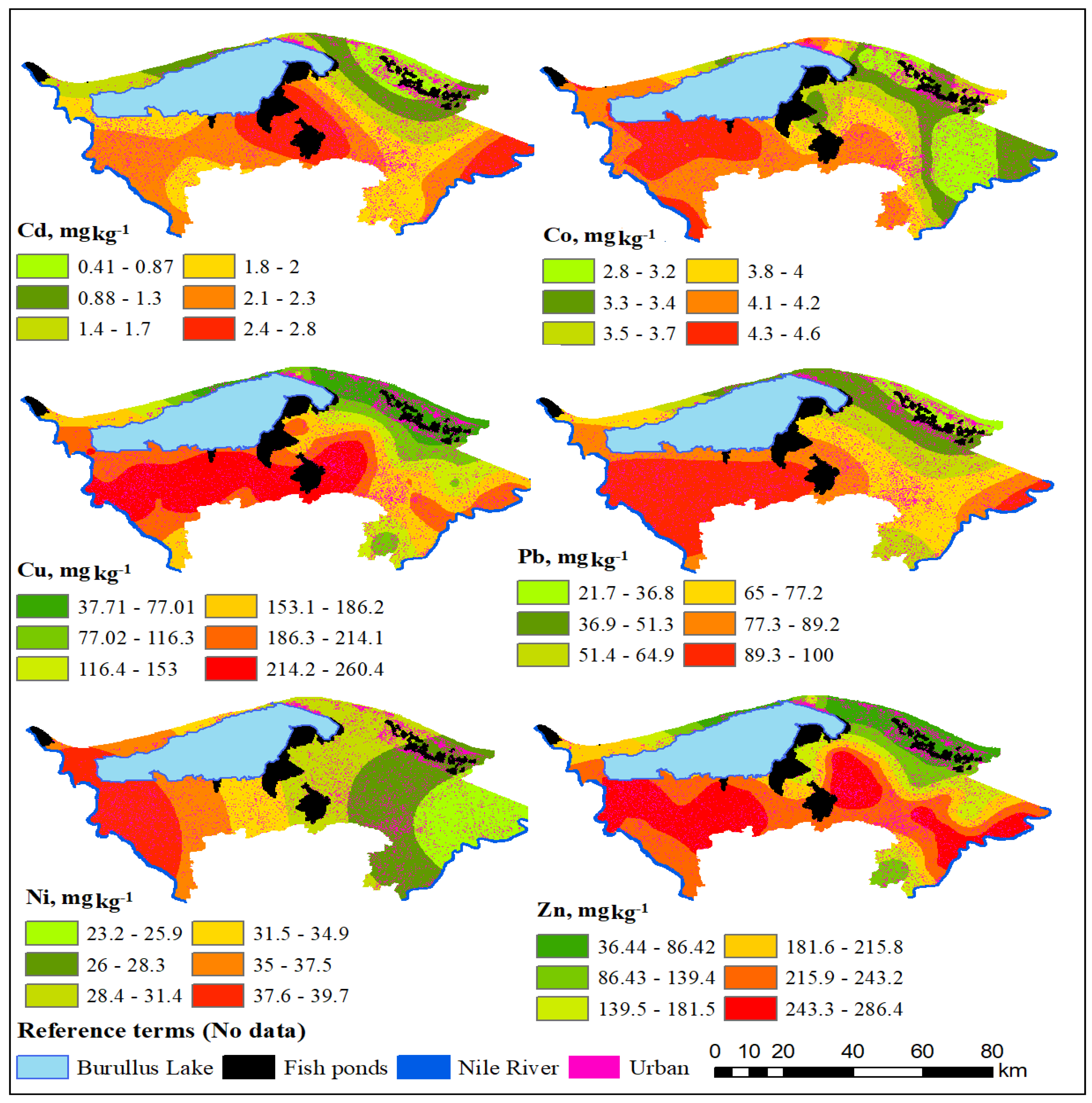
3.3. Metal Spatial Variability in Soils

The spatial distribution of the six metals is depicted through semivariograms (Figure S2) and their parameters in

Table 4. Semivariogram parameters of the best-fitted ordinary kriging models used for predicting metal concentrations.

Variable	Transformation	Model	Nugget C0	Partial Sill C1	Sill C0 + C1	Nugget/ Sill	SPD	Range, km	Prediction Error
									ME	RMSE	MSE	RMSSE	ASE
Cd	None	Gaussian	0.418	0.604	1.022	0.409	Moderate	41.56	0.001	0.932	0.007	1.263	0.721
Co	Box-Cox	Circular	0.363	0.462	0.825	0.440	Moderate	29.95	0.000	0.918	0.002	1.213	0.744
Cu	Box-Cox	Exponential	0.003	0.008	0.011	0.236	Strong	75.69	0.004	0.077	0.040	1.172	0.067
Pb	Box-Cox	Gaussian	201.770	1064.700	1266.470	0.159	Strong	66.57	0.010	20.300	0.003	1.269	15.838
Ni	Log	Gaussian	0.022	0.077	0.099	0.227	Strong	61.94	0.007	6.527	0.048	1.390	5.522
Zn	Box-Cox	Circular	0.002	0.010	0.012	0.145	Strong	44.79	0.004	0.081	0.043	1.300	0.061

SPD, spatial dependence; ME, mean error; RMSE, root mean square error; MSE, mean standardized error; RMSSE; root mean square standardized error; ASE, average standardized error.

. The Kolmogorov–Smirnov test indicates that all metals did not show normal distribution, except Cd. Hence, Box-Cox and log transformations were applied before performing the interpolation. With lower errors, the Gaussian model was the best model fitted to the semivariograms of Cd, Pb, and Ni. The circular model was the best model fitted to the semivariograms of Co and Zn, while the exponential model was the best-fitted model to represent the Cu semivariogram. The cross-validation of semivariogram models (Figure S3) demonstrates good correlations between the predicted and measured concentrations of the six metals. The prediction errors (Table 4) reveal that values of ME and MSE for all applied models were close to zero, while the RMSSE values were close to unity. Moreover, the values of RMSE and ASE for each of the selected models were rather similar.

As shown in Table 4, a positive nugget effect (larger than 0), as well as a sill value, was reached for all the applied OK models. The nugget (C0)/sill (C0 + C) ratio define the spatial dependency (SPD), where ratios lesser than 0.25, 0.25–0.75, and above 0.75 indicate a strong, moderate, and weak SPD, respectively [25]. Hence, Cu, Pb, Ni, and Zn had a strong SPD, while Cd and Co had a moderate SPD. The semi-variogram range values varied considerably from 30 to 76 km. The range followed the order of Cu > Pb > Ni > Zn > Cd > Co. The prediction maps of the six metals computed from the semivariogram models are shown in Figure 3. The concentrations of Cd, Cu, Pb and Zn displayed a similar spatial pattern delineated by a northern zone with low values. The higher levels of these metals were mainly visible in the central and western parts and also in some zones in the east for Cd, Pb and Zn. On the other hand, concentrations of Co and Ni showed a different pattern. The lowest Co level occurred in eastern and northeastern parts across the studied area, while the highest level occurred mainly in the western parts besides small pockets in the south and northern parts. For Ni, the eastern and western parts characterized the lowest and highest levels, respectively.

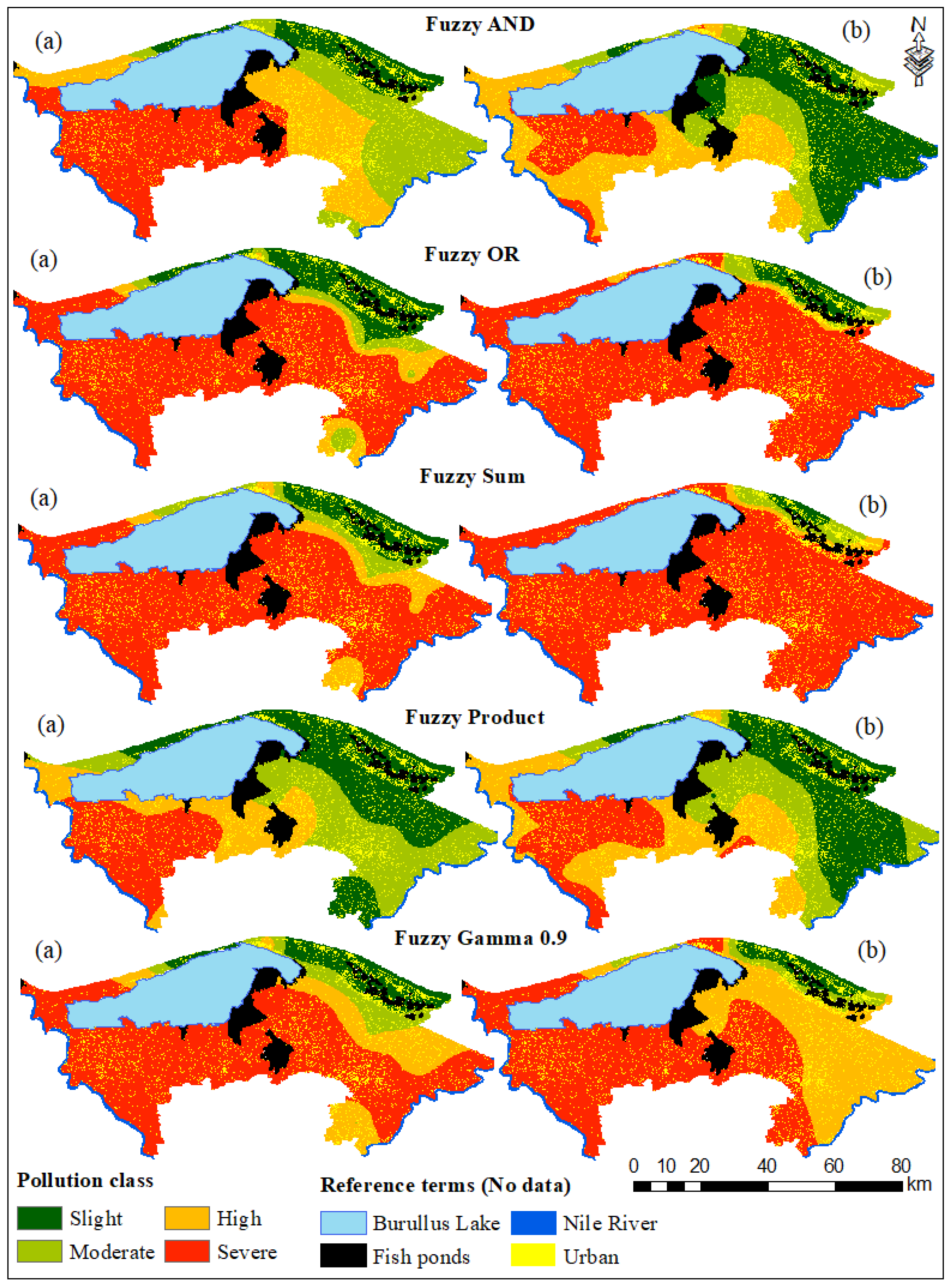
3.4. Modeling Soil Pollution

The overall pollution maps produced by overlaying the normalized layers (Figure S4) are shown in Figure 4. There were various classifications in response to different normalizations and overlay techniques. The ROC and AUC analysis, given in Figure 5, illustrates that pollution maps derived from the non-linearly normalized layers yielded higher AUC values than those from the linearly normalized ones. This trend occurred under all overlay operators, except for the fuzzy Product. For overlay operators, maps generated from the fuzzy Product showed the lowest AUC values, i.e., 0.551 and 0.571 (poor accuracy) when using the non-linearly and linearly normalized raster layers, respectively. On the other hand, maps developed by the fuzzy Sum operator displayed the highest AUC values for the linearly (AUC = 0.729; good accuracy) and non-linearly (AUC = 0.866; very good accuracy) normalized raster layers.

The highest prediction rates resulted from applying the fuzzy Sum and OR overlay to the non-linearly normalized raster layers with AUC values of 0.866 and 0.809, respectively, indicating a very good accuracy. As shown in Figure 4, results of the two models were highly similar, where the lower pollution levels occurred mainly in the northern parts. Based on the fuzzy Sum operator, about 92% of the studied soils were considered as severely polluted, 2% highly polluted, 3% moderately polluted, and 2% slightly polluted (

Table 5. Areas of soil pollution classes derived from the most suitable models.

Normalization	Operator	Class	Area
			ha	%
Non-linear	Fuzzy Sum	Slight	5219	1.83
		Moderate	9868	3.46
		High	6702	2.35
		Severe	263,417	92.36
	Fuzzy OR	Slight	15,629	5.48
		Moderate	8539	2.99
		High	6156	2.16
		Severe	254,882	89.37

). On the other hand, under the fuzzy OR operator, severely, highly, moderately, and slightly polluted soils occupied about 89%, 2%, 3%, and 5% of the total cultivated lands, respectively.

4. Discussion

4.1. Metal Concentrations in Soils

Soil metal content reflects the level of severity as the presence of metal toxicants in soils is not hazardous unless they surpass certain levels. The earth’s natural element content has been accepted as a reference value to assess potential metal hazards [49,55]. Accordingly, Co in all soils showed a safe level, while the remaining metals would pose potential risks as reported in an earlier study in the northern Nile Delta [56]. However, different metal hazards have been reported in other studies in the same region. For instance, Rinklebe and Shaheen [57] studied distributions of Co, Cu, Ni, and Zn in five soil profiles developed on fluvial and lacustrine deposits. In all horizons, they found metal content above the threshold limits, except Cu which was below 55 mg kg⁻¹. Moreover, Abuzaid and Jahin [58] reported content of Cu and Pb in three depth intervals (0–30, 30–60, and 60–90 cm) within the safe limits, while corresponding values for Cd, Co, Ni, and Zn were above those limits, except in soils developed on sand deposits. Hence, metal content in all horizons of the northern Nile Delta soils are likely affected by parent materials, soil type, and human activities as concluded in previous studies [58,59,60].

The coefficient of variation (CV) value indicates the degree of discrete distributions of metal content in soils, and also reflects metal variability in response to natural and anthropic factors [25,44]. The intermediate metal heterogeneity, as in the current study, is probably due to similar environmental conditions and cropping systems. Soil developed on alluvial deposits (from the Nile River) prevail the entire area, except in the northern parts that are dominated by soils developed on marine and lacustrine deposits. In addition, rice cultivation is the main land use type in the northern Nile Delta region [61], and thus cropping systems in the studied area seems to be rather similar.

The significant build-up in metal content in the topsoil demonstrates that all metals did not show any downward migration. These findings are in line with a previous study in the northern Nile Delta [56] and a global study in an arid area of northwest China [44]. Generally, the topsoil is more vulnerable to human interference, and thus it can be easily enriched by metal toxicants [44,62]. Moreover, the vertical movement of PTMs in many arid and semi-arid regions is significantly governed by physicochemical properties of the soil profile [58,63]. As shown in Table 1, key soil properties (OM, pH, clay, Fe, and Mn) tended to decrease with depth, and thus the metal content followed the same trend.

4.2. Metal Relationships in Soils

The correlation results indicate that soil properties played crucial roles in metal accumulation. The pH rise increases the negative charge of soil organic and inorganic colloids, enhancing soil capacity to hold metal cations by electrostatic sorption [64]. The metal correlations with EC suggest that Cd, Cu, Pb, and Zn formed soluble complexes with inorganic and organic ligands in soils, while Co and Ni occurred in more stable complexes [65]. The positive metal correlations with OM affirm that organic compounds are significant reservoirs for metals in soils [62]. Moreover, organic agrochemicals are likely to be the main source of metal toxicants [66]. The metal correlations with fine-earth reveal that, except for Cd, they were related to silt- and clay-sized fractions, implying the strong bound to phyllosilicate minerals [64,65]. The positive correlations of Cd, Co, and Pb with Fe and Mn indicate that they might be adsorbed on or co-precipitated with Fe and Mn oxides [65]. The metal interactions among each other reveal similar geochemical behavior or common source of Cd, Cu, Pb, Ni, and Zn, which differed from Co.

The PCA has been accepted as a powerful tool to identify potential sources of metal toxicants in agricultural soils [14,56,59]. In our study, three PCs reflecting possible origins and controlling mechanisms were identified. PC1 could denote the contribution of human activities, mainly agronomic practices. This could be affirmed by the strong correlations of OM, Cd, Cu, Pb, and Zn, and the moderate correlation of Ni under this PC. At the same time, the mean concentrations of these PTMs were far away from their lithogenic contents. These findings are rather similar to those obtained by Emam and Soliman [59], who reported anthropic origins for Cd, Cu, Pb, and Zn in soils of the northern Nile Delta region.

PC2 could reflect the contribution of the Nile Delta alluvial sediments since inherent soil properties (sand, silt, and clay) were strongly correlated to this PC. The strong positive loadings of clay and silt coupled with the strong negative loading of sand indicate that the origin of sand was completely different from the source of silt and clay as concluded by Garzanti et al. [67]. The moderate positive loading of Ni in this PC indicates that the Nile sediments might also enrich the soils with Ni. Normally, Ni occurs in ultramafic rocks (serpentine) [49] that dominate the Nile Delta sediments [67].

PC3 could refer to the predominance of ferromagnesian minerals since strong positive loadings of Fe, Mn, and Co occurred. These findings are consistent with earlier works [58,59,68], which confirmed the similar source of Fe, Mn, and Co in the northern Nile Delta soils. Naturally, Co and Mn are found in the ferromagnesian minerals (olivine, hornblende, and augite) since their respective divalent radii allow them to substitute readily for Fe (II) and Mg (II). Thus, the greatest content of Mn and Co is mostly found in basic (basalt) and ultrabasic (serpentine) rocks [69]. Consequently, the Nile sediments, rich in basalt and serpentine rocks [67], are an important source for these metals in the northern Nile Delta region.

4.3. Metal Spatial Variability in Soils

The Gaussian, circular, and exponential semivariogram models were accepted to simulate the spatial structure of the studied metals. Comparing these findings with a previous study in the Nile Valley of Egypt, Hammam et al. [14] reported that the best-fitted OK models were stable models for Cd, Co, and Cu, Gaussian model for Pb, and spherical model for Zn. In an arid area of northwest China, Wang et al. [15] found that the spherical model was the most suitable to represent the Cu semivariogram, while the Gaussian model was proper for Pb and Zn. Chiefly, selecting the best-fitted methods depends on the comparison of cross-validation metrics, i.e., ME, RMSE, MSE, RMSSE, and ASE [24,26].

The applied OK models in the current work could achieve the minimum ME and MSE, RMSSE near unity, and similar values for each of RMSE and ASE, providing acceptable estimations for the non-sampled sites [26,47]. The models with ME and MSE close to zero offer unbiased prediction [24]; meanwhile, those of positive or negative ME values underestimate or overestimate data variability, respectively [70]. Moreover, the RMSSE near unity also reveals high prediction accuracy for the applied model [26,47].

The spatial structure of the PTMs could be depicted through the semivariogram parameters: nugget effect, sill value, range, and nugget to sill ratio. The nugget and sill express the random and general variance of the regional variable, respectively, while the range denotes the extent of spatial autocorrelation [22]. The positive nugget value, as in our work, stems from the effects of sampling error (limited or dense points), measurement error, and the presence of data outliers [25]. However, achieving a sill value confirms that data have a spatial structure and can be simulated via semivariogram models [46]. The nugget/sill ratio reveals the effects of human and soil factors on the SPD of metals. According to recent studies [25,26,46], weak SPD is mainly due to extrinsic factors (agronomic practices), while strong SPD is due to intrinsic factors (soil properties). Hence, the strong SPD of Cu, Pb, Ni, and Zn could be attributed to variations of soil parent materials, while the moderate SPD of Cd and Co could be due to the mutual effects of agricultural practices and soil properties.

The semivariogram range determines the maximum distance of correlation between sampling points [70], where high range values reflect a large-scale heterogeneity and vice versa [46]. Over large areas, the higher range value of a soil property denotes a stronger combined effect of natural and human factors [25]. Thus, the mutual effect of soil properties and agronomic practices is more apparent for Cu but less important for Co, which had the largest and lowest semivariogram range values, respectively. According to Goenster-Jordan et al. [46] and Dad and Ul Shafiq [25], the profound assessment of spatial heterogeneity entails a sampling distance less than half of the semivariogram range. Therefore, it is recommended to conduct further investigations in the study area and similar regions using soil sampling distances of about or even smaller than 21, 15, 38, 33, 31, and 22 km for Cd, Co, Cu, Pb, Ni, and Zn, respectively.

The distribution maps revealed that the lowest metal concentrations were in the northern parts, where the soils had a light texture (loamy sand to sand). These results are similar to those obtained by Abuzaid and Jahin [58], who reported that the lowest concentrations of Cd, Co, Cu, Pb, Ni, and Zn in the northern Nile Delta soils occurred in the sand sheet unit. Normally, the coarse-textured soils developed on sandstone or sand drift contain lesser amounts of PTMs compared with fine-textured soils [65,66]. The sandstones contain the lowest amounts of metals and metalloids [49,71]. In addition, due to the lack of active adsorption sites, coarse particles are not able to hold or adsorb significant amounts of metals added to the soils [64,65].

4.4. Modeling Soil Metal Pollution

The overall soil pollution maps reflect the different performances of FMFs (linear and non-linear) and fuzzy overlay operators (And, OR, Sum, Product, and Gamma). Generally, linear functions depend on simple calculations, while non-linear functions use more complicated mathematical algorithms [72]. Hence, non-linear functions can provide a deeper knowledge of how each indicator affects the soil ecosystem [73]. This interpretation could explain the superiority of the non-linearly normalized layers over the linearly normalized ones under different fuzzy overlay operators.

The effects of various fuzzy operators could also be seen since each technique can portray the interactions of the memberships in significantly different ways [33]. The fuzzy And as well as fuzzy OR offers an intersection operator, which extracts the minimum and maximum membership values of the input layers, respectively [32]. Thus, they produce extreme results as they focus on certain pixels but ignore the remaining cells [31]. However, the fuzzy OR overlay is preferred when assessing environmental hazards since it delineates the most serious factors [32,74]. This suggestion could be supported by the higher prediction accuracy for the fuzzy OR operator than the fuzzy And operator under the linear and non-linear FMFs.

The fuzzy Sum and Product operators consider all pixels of the input layers, overlaying them in two different manners [32]. The fuzzy algebraic sum is an increasing operator, where integrating the multiple input layers is more important than any of them alone [33]. Since the overall soil pollution relies on multiple metals, this operator yielded the highest prediction rates when using either linearly or non-linearly normalized layers. It is unlikely that the fuzzy algebraic product is a deceasing operator, where combining the multiple layers is less important than any of them alone [33]. Despite the output map being affected by all pixels, multiplying the effective factors weakens each other [74], rendering such a technique more restricted [33]. This could interpret the poor prediction accuracy of this operator under the two normalization methods.

The fuzzy Gamma operator can simultaneously combine the fuzzy Sum and Product operators. Hence, it provides a flexible tool to adjust the increasing and decreasing tendencies of the two operators [32]. The fuzzy Gamma has been reported as the best fuzzy overlay technique for suitability analysis [33,47,48] and wind erosion hazards [31,32]. However, in our work, the fuzzy Gamma overlay had a moderate prediction rate under the two normalization methods. This could be attributed mainly to the use of different parameters and membership functions.

Results of the fuzzy Sum overlay were highly similar to those of the fuzzy OR overlay under the two normalization methods. This might be due to the monotonically increasing membership of metal layers since an increase in the metal content enhances the occurrence of soil pollution [4,13]. The very good prediction accuracy obtained from applying the fuzzy Sum and OR overlay to the non-linearly normalized layers illustrates that both models were highly suitable to predict soil pollution in the studied area. The high accuracy is likely due to the deeper analysis of metal contributions to soil pollution achieved by the non-linear functions [72,73] in addition to the sensitivity of the two operators to the increasing tendency characterizing metal memberships [32,74]. However, the fuzzy Sum operator is considered the best model in terms of prediction accuracy (86.6%), which should be adopted for decision-making in the studied area and similar regions. According to this model, more than 92% of the investigated soils were severely polluted, posing potential environmental and health risks. Hence, future remediation studies should be adopted to suggest proper soil and crop management strategies.

5. Conclusions

In the present work, a novel spatial assessment of soil metal pollution on a regional scale was adopted in an arid area (north Nile Delta, Egypt). This was achieved through integrating geostatistics with fuzzy logic techniques under the GIS platform. The OK models could adequately depict the spatial structure of six PTMs in soils. The best-fitted semivariogram models were Gaussian for Cd, Pb, and Ni, circular for Co and Zn, and exponential for Cu. Four metals (Cu, Pb, Ni, and Zn) showed a strong SPD, reflecting variations of soil properties; meanwhile, Cd and Co displayed a moderate SPD, indicating mutual effects of human and natural factors. The ROC and AUC analysis revealed different prediction accuracies of the developed soil pollution maps. The non-linear FMFs were superior to the linear functions for modeling soil metal pollution. Under the two normalization methods, the fuzzy Sum and fuzzy Product overlay operators resulted in the highest and lowest prediction accuracy, respectively. Overall, the highest prediction accuracy (AUC = 0.866; very good) presented when applying the fuzzy Sum overly to the non-linearly normalized raster layers. This model could accomplish a success rate of 86.6%, implying that it should be adopted for decision-making in the studied area. According to this model, nearly 92% of the studied soils were severely polluted, posing potential ecological and health risks. Hence, great attention should be paid to immediate soil remediation scenarios. Our study would increase insight into soil metal pollution on a regional scale. Yet, it is advocated to design proper sampling distances to obtain higher geostatistical precision and efficient metal mapping in similar regions.

References

1. Ferreira, C.S.S.; Seifollahi-Aghmiuni, S.; Destouni, G.; Ghajarnia, N.; Kalantari, Z. Soil degradation in the European Mediterranean region: Processes, status and consequences. Sci. Total Environ. 2022, 805, 150106. [Google Scholar] [CrossRef] [PubMed]
2. Dubey, P.K.; Singh, A.; Raghubanshi, A.; Abhilash, P. Steering the restoration of degraded agroecosystems during the United Nations Decade on Ecosystem Restoration. J. Environ. Manag. 2020, 280, 111798. [Google Scholar] [CrossRef] [PubMed]
3. Saljnikov, E.; Lavrishchev, A.; Römbke, J.; Rinklebe, J.; Scherber, C.; Wilke, B.-M.; Tóth, T.; Blum, W.E.H.; Behrendt, U.; Eulenstein, F.; et al. Understanding and monitoring chemical and biological soil degradation. In Advances in Understanding Soil Degradation; Saljnikov, E., Mueller, L., Lavrishchev, A., Eulenstein, F., Eds.; Springer International Publishing: Cham, Switzerland, 2022; pp. 75–124. [Google Scholar]
4. Kumar, V.; Pandita, S.; Setia, R. A meta-analysis of potential ecological risk evaluation of heavy metals in sediments and soils. Gondwana Res. 2022, 103, 487–501. [Google Scholar] [CrossRef]
5. Chen, L.; Beiyuan, J.; Hu, W.; Zhang, Z.; Duan, C.; Cui, Q.; Zhu, X.; He, H.; Huang, X.; Fang, L. Phytoremediation of potentially toxic elements (PTEs) contaminated soils using alfalfa (Medicago sativa L.): A comprehensive review. Chemosphere 2022, 293, 133577. [Google Scholar] [CrossRef]
6. Daulta, R.; Prakash, M.; Goyal, S. Metal content in soils of Northern India and crop response: A review. Int. J. Environ. Sci. Technol. 2022; in press. [Google Scholar] [CrossRef]
7. Nowicka, B. Heavy metal-induced stress in eukaryotic algae-mechanisms of heavy metal toxicity and tolerance with particular emphasis on oxidative stress in exposed cells and the role of antioxidant response. Environ. Sci. Pollut. Res. 2022, 29, 16860–16911. [Google Scholar] [CrossRef]
8. Yang, Z.; Yang, F.; Liu, J.-L.; Wu, H.-T.; Yang, H.; Shi, Y.; Liu, J.; Zhang, Y.-F.; Luo, Y.-R.; Chen, K.-M. Heavy metal transporters: Functional mechanisms, regulation, and application in phytoremediation. Sci. Total. Environ. 2021, 809, 151099. [Google Scholar] [CrossRef]
9. Abuzaid, A.S.; Bassouny, M.; Jahin, H.; Abdelhafez, A. Stabilization of lead and copper in a contaminated Typic Torripsament soil using humic substances. CLEAN Soil Air Water 2019, 47, 1800309. [Google Scholar] [CrossRef]
10. Song, P.; Xu, D.; Yue, J.; Ma, Y.; Dong, S.; Feng, J. Recent advances in soil remediation technology for heavy metal contaminated sites: A critical review. Sci. Total Environ. 2022, 838, 156417. [Google Scholar] [CrossRef]
11. Abuzaid, A.S.; Jahin, H.S. Implications of irrigation water quality on shallow groundwater in the Nile Delta of Egypt: A human health risk prospective. Environ. Technol. Innov. 2021, 22, 101383. [Google Scholar] [CrossRef]
12. Abbas, H.; Abuzaid, A.S.; Jahin, H.; Kasem, D. Assessing the quality of untraditional water sources for irrigation purposes in Al-Qalubiya Governorate, Egypt. Egypt. J. Soil Sci. 2020, 60, 157–166. [Google Scholar] [CrossRef]
13. Yang, H.; Wang, F.; Yu, J.; Huang, K.; Zhang, H.; Fu, Z. An improved weighted index for the assessment of heavy metal pollution in soils in Zhejiang, China. Environ. Res. 2020, 192, 110246. [Google Scholar] [CrossRef] [PubMed]
14. Hammam, A.A.; Mohamed, W.S.; Sayed, S.E.-E.; Kucher, D.E.; Mohamed, E.S. Assessment of Soil Contamination Using GIS and Multi-Variate Analysis: A Case Study in El-Minia Governorate, Egypt. Agronomy 2022, 12, 1197. [Google Scholar] [CrossRef]
15. Wang, N.; Guan, Q.; Sun, Y.; Wang, B.; Ma, Y.; Shao, W.; Li, H. Predicting the spatial pollution of soil heavy metals by using the distance determination coefficient method. Sci. Total. Environ. 2021, 799, 149452. [Google Scholar] [CrossRef] [PubMed]
16. Ahmad, N.; Pandey, P. Spatio-Temporal Distribution, Ecological Risk Assessment, and Multivariate Analysis of Heavy Metals in Bathinda District, Punjab, India. Water Air Soil Pollut. 2020, 231, 431. [Google Scholar] [CrossRef]
17. Gozukara, G.; Acar, M.; Ozlu, E.; Dengiz, O.; Hartemink, A.E.; Zhang, Y. A soil quality index using Vis-NIR and pXRF spectra of a soil profile. Catena 2022, 211, 105954. [Google Scholar] [CrossRef]
18. Gozukara, G. Rapid land use prediction via portable X-ray fluorescence (pXRF) data on the dried lakebed of Avlan Lake in Turkey. Geoderma Reg. 2021, 28, e00464. [Google Scholar] [CrossRef]
19. Evans, N.; Van Ryswyk, H.; Huertos, M.L.; Srebotnjak, T. Robust spatial analysis of sequestered metals in a Southern California Bioswale. Sci. Total Environ. 2018, 650, 155–162. [Google Scholar] [CrossRef]
20. Jin, Z.; Zhang, L.; Lv, J.; Sun, X. The application of geostatistical analysis and receptor model for the spatial distribution and sources of potentially toxic elements in soils. Environ. Geochem. Health 2020, 43, 407–421. [Google Scholar] [CrossRef]
21. Zhen, J.; Pei, T.; Xie, S. Kriging methods with auxiliary nighttime lights data to detect potentially toxic metals concentrations in soil. Sci. Total. Environ. 2019, 659, 363–371. [Google Scholar] [CrossRef]
22. Golden, N.; Zhang, C.; Potito, A.; Gibson, P.J.; Bargary, N.; Morrison, L. Use of ordinary cokriging with magnetic susceptibility for mapping lead concentrations in soils of an urban contaminated site. J. Soils Sediments 2019, 20, 1357–1370. [Google Scholar] [CrossRef]
23. Shi, C.; Wang, Y. Non-parametric machine learning methods for interpolation of spatially varying non-stationary and non-Gaussian geotechnical properties. Geosci. Front. 2020, 12, 339–350. [Google Scholar] [CrossRef]
24. Abuzaid, A.S.; Mazrou, Y.S.A.; El Baroudy, A.A.; Ding, Z.; Shokr, M.S. Multi-Indicator and Geospatial Based Approaches for Assessing Variation of Land Quality in Arid Agroecosystems. Sustainability 2022, 14, 5840. [Google Scholar] [CrossRef]
25. Dad, J.M.; Shafiq, M.U. Spatial variability and delineation of management zones based on soil micronutrient status in apple orchard soils of Kashmir valley, India. Environ. Monit. Assess. 2021, 193, 797. [Google Scholar] [CrossRef]
26. Sebei, A.; Chaabani, A.; Abdelmalek-Babbou, C.; Helali, M.A.; Dhahri, F.; Chaabani, F. Evaluation of pollution by heavy metals of an abandoned Pb-Zn mine in northern Tunisia using sequential fractionation and geostatistical mapping. Environ. Sci. Pollut. Res. 2020, 27, 43942–43957. [Google Scholar] [CrossRef]
27. Zhang, X.; She, D.; Wang, G.; Huang, X. Source identification of soil elements and risk assessment of trace elements under different land uses on the Loess Plateau, China. Environ. Geochem. Health 2020, 43, 2377–2392. [Google Scholar] [CrossRef]
28. Lermi, A.; Kelebek, G.; Sunkari, E.D. Assessment of the concentrations, distributions, and sources of potentially toxic elements in the soil–water–plant system in the Bolkar mining district, Niğde, south-central Turkey. Arab. J. Geosci. 2022, 15, 886. [Google Scholar] [CrossRef]
29. Wang, H.; Zhang, H.; Liu, Y. Using a posterior probability support vector machine model to assess soil quality in Taiyuan, China. Soil Tillage Res. 2018, 185, 146–152. [Google Scholar] [CrossRef]
30. Ghiasvand, F.; Babaei, A.A.; Yazdani, M.; Birgani, Y.T. Spatial modeling of environmental vulnerability in the biggest river in Iran using geographical information systems. J. Environ. Health Sci. Eng. 2021, 19, 1069–1074. [Google Scholar] [CrossRef]
31. Saadoud, D.; Hassani, M.; Peinado, F.J.M.; Guettouche, M.S. Application of fuzzy logic approach for wind erosion hazard mapping in Laghouat region (Algeria) using remote sensing and GIS. Aeolian Res. 2018, 32, 24–34. [Google Scholar] [CrossRef]
32. Razifard, M.; Shoaei, G.; Zare, M. Application of fuzzy logic in the preparation of hazard maps of landslides triggered by the twin Ahar-Varzeghan earthquakes (2012). Bull. Eng. Geol. Environ. 2018, 78, 223–245. [Google Scholar] [CrossRef]
33. Lewis, S.M.; Fitts, G.; Kelly, M.; Dale, L. A fuzzy logic-based spatial suitability model for drought-tolerant switchgrass in the United States. Comput. Electron. Agric. 2014, 103, 39–47. [Google Scholar] [CrossRef]
34. Yang, Y.; Zhou, Z.; Bai, Y.; Cai, Y.; Chen, W. Risk Assessment of Heavy Metal Pollution in Sediments of the Fenghe River by the Fuzzy Synthetic Evaluation Model and Multivariate Statistical Methods. Pedosphere 2016, 26, 326–334. [Google Scholar] [CrossRef]
35. Islam, A.R.M.T.; Kabir, M.M.; Faruk, S.; Al Jahin, J.; Doza, B.; Alam, D.U.; Bahadur, N.M.; Mohinuzzaman, M.; Fatema, K.J.; Rahman, M.S.; et al. Sustainable groundwater quality in southeast coastal Bangladesh: Co-dispersions, sources, and probabilistic health risk assessment. Environ. Dev. Sustain. 2021, 23, 18394–18423. [Google Scholar] [CrossRef]
36. Soil Survey Staff. Keys to Soil Taxonomy, 12th ed.; United States Department of Agriculture, Natural Resources Conservation Service: Washington, DC, USA, 2014.
37. Prăvălie, R.; Bandoc, G.; Patriche, C.; Sternberg, T. Recent changes in global drylands: Evidences from two major aridity databases. Catena 2019, 178, 209–231. [Google Scholar] [CrossRef]
38. CONCO-Coral/EGPC. Geologic Map of Egypt, Scale 1:500,000; Conoco-Coral and Egyptian General Petroleum Company (EGPC): Cairo, Egypt, 1987. [Google Scholar]
39. Abuzaid, A.S.; Abdelatif, A.D. Assessment of desertification using modified MEDALUS model in the north Nile Delta, Egypt. Geoderma 2021, 405, 115400. [Google Scholar] [CrossRef]
40. FAO. Guidelines for Soil Description, 4th ed.; Food and Agriculture Organization of the United Nations (FAO): Rome, Italy, 2006. [Google Scholar]
41. Soil Survey Staff. Soil Survey Staff. Soil survey field and laboratory methods manual. In Soil Survey Investigations Report No. 51, Version 2.0; Burt, R., Soil Survey Staff, Eds.; U.S. Department of Agriculture, Natural Resources Conservation Service: Washington, DC, USA, 2014. [Google Scholar]
42. USEPA. Test methods for evaluating solid waste. In IA: Laboratory Manual Physical/Chemical Methods, SW 846, 3rd ed.; U.S. Gov. Print. Office: Washington, DC, USA, 1995. [Google Scholar]
43. Abuzaid, A.S.; Jahin, H.S. Combinations of multivariate statistical analysis and analytical hierarchical process for indexing surface water quality under arid conditions. J. Contam. Hydrol. 2022, 248, 104005. [Google Scholar] [CrossRef]
44. Fan, S.; Wang, X.; Lei, J.; Ran, Q.; Ren, Y.; Zhou, J. Spatial distribution and source identification of heavy metals in a typical Pb/Zn smelter in an arid area of northwest China. Hum. Ecol. Risk Assess. 2019, 25, 1661–1687. [Google Scholar] [CrossRef]
45. Santra, P.; Kumar, M.; Panwar, N.; Yadav, R. Digital soil mapping: The future need of sustainable soil management. In Geospatial Technologies for Crops and Soils; Mitran, T., Meena, R., Chakraborty, A., Eds.; Springer: Singapore, 2021; pp. 319–355. [Google Scholar]
46. Goenster-Jordan, S.; Jannoura, R.; Jordan, G.; Buerkert, A.; Joergensen, R.G. Spatial variability of soil properties in the floodplain of a river oasis in the Mongolian Altay Mountains. Geoderma 2018, 330, 99–106. [Google Scholar] [CrossRef]
47. Mallik, S.; Mishra, U.; Paul, N. Groundwater suitability analysis for drinking using GIS based fuzzy logic. Ecol. Indic. 2020, 121, 107179. [Google Scholar] [CrossRef]
48. Mustafiz, R.B.; Noguchi, R.; Ahamed, T. Calorie-based seasonal multicrop land suitability analysis using GIS and remote sensing for regional food nutrition security in Bangladesh. In Remote Sensing Application: Regional Perspectives in Agriculture and Forestry; Ahamed, T., Ed.; Springer Nature: Singapore, 2022; pp. 25–64. [Google Scholar]
49. Kabata-Pendias, A. Trace Elements in Soils and Plants; CRC Press, Taylor and Francis Group, LLC: Boca Raton, FL, USA, 2011. [Google Scholar]
50. Akbari, S.; Ramazi, H.; Ghezelbash, R.; Maghsoudi, A. Geoelectrical integrated models for determining the geometry of karstic cavities in the Zarrinabad area, west of Iran: Combination of fuzzy logic, C-A fractal model and hybrid AHP-TOPSIS procedure. Carbonates Evaporites 2020, 35, 56. [Google Scholar] [CrossRef]
51. Daviran, M.; Maghsoudi, A.; Cohen, D.R.; Ghezelbash, R.; Yilmaz, H. Assessment of Various Fuzzy c-Mean Clustering Validation Indices for Mapping Mineral Prospectivity: Combination of Multifractal Geochemical Model and Mineralization Processes. Nat. Resour. Res. 2019, 29, 229–246. [Google Scholar] [CrossRef]
52. Sam, K. Modeling the effectiveness of natural and anthropogenic disturbances on forest health in Buxa Tiger Reserve, India, using fuzzy logic and AHP approach. Model. Earth Syst. Environ. 2021, 8, 2261–2276. [Google Scholar] [CrossRef]
53. Pathak, D.; Maharjan, R.; Maharjan, N.; Shrestha, S.R.; Timilsina, P. Evaluation of parameter sensitivity for groundwater potential mapping in the mountainous region of Nepal Himalaya. Groundw. Sustain. Dev. 2021, 13, 100562. [Google Scholar] [CrossRef]
54. Al-Abadi, A.M.; Ghalib, H.B.; Al-Mohammdawi, J.A. Delineation of Groundwater Recharge Zones in Ali Al-Gharbi District, Southern Iraq Using Multi-criteria Decision-making Model and GIS. J. Geovisualization Spat. Anal. 2020, 4, 9. [Google Scholar] [CrossRef]
55. Khan, S.; Naushad, M.; Lima, E.C.; Zhang, S.; Shaheen, S.M.; Rinklebe, J. Global soil pollution by toxic elements: Current status and future perspectives on the risk assessment and remediation strategies—A review. J. Hazard. Mater. 2021, 417, 126039. [Google Scholar] [CrossRef]
56. Abuzaid, A.S.; Bassouny, M.A. Total and DTPA-extractable forms of potentially toxic metals in soils of rice fields, north Nile Delta of Egypt. Environ. Technol. Innov. 2020, 18, 100717. [Google Scholar] [CrossRef]
57. Rinklebe, J.; Shaheen, S.M. Geochemical distribution of Co, Cu, Ni, and Zn in soil profiles of Fluvisols, Luvisols, Gleysols, and Calcisols originating from Germany and Egypt. Geoderma 2017, 307, 122–138. [Google Scholar] [CrossRef]
58. Abuzaid, A.S.; Jahin, H. Profile Distribution and Source Identification of Potentially Toxic Elements in North Nile Delta, Egypt. Soil Sediment Contam. Int. J. 2019, 28, 582–600. [Google Scholar] [CrossRef]
59. Emam, W.W.M.; Soliman, K.M. Geospatial analysis, source identification, contamination status, ecological and health risk assessment of heavy metals in agricultural soils from Qallin city, Egypt. Stoch. Hydrol. Hydraul. 2021, 36, 2437–2459. [Google Scholar] [CrossRef]
60. Aitta, A.; El-Ramady, H.; Alshaal, T.; El-Henawy, A.; Shams, M.; Talha, N.; Elbehiry, F.; Brevik, E.C. Seasonal and Spatial Distribution of Soil Trace Elements around Kitchener Drain in the Northern Nile Delta, Egypt. Agriculture 2019, 9, 152. [Google Scholar] [CrossRef] [Green Version]
61. Elbasiouny, H.; Elbehiry, F. Rice production in Egypt: The challenges of climate change and water deficiency. In Climate Change Impacts on Agriculture and Food Security in Egypt: Land and Water Resources—Smart Farming—Livestock, Fishery, and Aquaculture; Omran, E.-S.E., Negm, A., Eds.; Springer International Publishing: Cham, Switzerland, 2020; pp. 295–319. [Google Scholar]
62. Preston, W.; da Silva, Y.J.; Nascimento, C.W.D.; da Cunha, K.P.; Silva, D.J.; Ferreira, H.A. Soil contamination by heavy metals in vineyard of a semiarid region: An approach using multivariate analysis. Geoderma Reg. 2016, 7, 357–365. [Google Scholar] [CrossRef] [Green Version]
63. Irshad, S.; Liu, G.; Yousaf, B.; Ali, M.U.; Ahmed, R.; Rehman, A.; Rashid, M.S.; Mahfooz, Y. Geochemical fractionation and spectroscopic fingerprinting for evaluation of the environmental transformation of potentially toxic metal(oid)s in surface–subsurface soils. Environ. Geochem. Health 2021, 43, 4329–4343. [Google Scholar] [CrossRef] [PubMed]
64. Rate, A.W. (Ed.) Inorganic contaminants in urban soils. In Urban Soils: Principles and Practice; Springer International Publishing: Cham, Switzerland, 2022; pp. 153–199. [Google Scholar]
65. Nieder, R.; Benbi, D.; Reichl, F. Role of potentially toxic elements in soils. In Soil Components and Human Health; Springer: Dordrecht, The Netherlands, 2018; pp. 375–450. [Google Scholar]
66. Elbana, T.; Gaber, H.; Kishk, F. Soil chemical pollution and sustainable agriculture. In The Soils of Egypt; El-Ramady, H., Alshaal, T., Bakr, N., Elbana, T., Mohamed, E., Belal, A.A., Eds.; Springer International Publishing: Cham, Switzerland, 2019; pp. 187–200. [Google Scholar]
67. Garzanti, E.; Andò, S.; Limonta, M.; Fielding, L.; Najman, Y. Diagenetic control on mineralogical suites in sand, silt, and mud (Cenozoic Nile Delta): Implications for provenance reconstructions. Earth Sci. Rev. 2018, 185, 122–139. [Google Scholar] [CrossRef]
68. Shaheen, S.M.; Antoniadis, V.; Kwon, E.; Song, H.; Wang, S.-L.; Hseu, Z.-Y.; Rinklebe, J. Soil contamination by potentially toxic elements and the associated human health risk in geo- and anthropogenic contaminated soils: A case study from the temperate region (Germany) and the arid region (Egypt). Environ. Pollut. 2020, 262, 114312. [Google Scholar] [CrossRef]
69. Uren, N.C. Cobalt and manganese. In Heavy Metals in Soils: Trace Metals and Metalloids in Soils and Their Bioavailability; Alloway, B., Ed.; Springer: Dordrecht, The Netherlands, 2013; pp. 335–366. [Google Scholar]
70. Kumar, P.; Kumar, P.; Shukla, A. Spatial modeling of some selected soil nutrients using geostatistical approach for Jhandutta Block (Bilaspur District), Himachal Pradesh, India. Agric. Res. 2021, 10, 262–273. [Google Scholar] [CrossRef]
71. Alloway, B.J. (Ed.) Sources of heavy metals and metalloids in soils. In Heavy Metals in Soils: Trace Metals and Metalloids in Soils and Their Bioavailability; Springer: Dordrecht, The Netherlands, 2013; pp. 11–50. [Google Scholar]
72. Zhou, Y.; Ma, H.; Xie, Y.; Jia, X.; Su, T.; Li, J.; Shen, Y. Assessment of soil quality indexes for different land use types in typical steppe in the loess hilly area, China. Ecol. Indic. 2020, 118, 106743. [Google Scholar] [CrossRef]
73. Mamehpour, N.; Rezapour, S.; Ghaemian, N. Quantitative assessment of soil quality indices for urban croplands in a calcareous semi-arid ecosystem. Geoderma 2020, 382, 114781. [Google Scholar] [CrossRef]
74. Aghda, S.M.F.; Bagheri, V.; Razifard, M. Landslide Susceptibility Mapping Using Fuzzy Logic System and Its Influences on Mainlines in Lashgarak Region, Tehran, Iran. Geotech. Geol. Eng. 2018, 36, 915–937. [Google Scholar]
Figure 1. Location maps of the study area.
Agronomy 13 00161 g001
Figure 2. Geological map and soil profile locations.
Agronomy 13 00161 g002
Figure 3. Spatial distribution maps of the studied elements based on the weighted mean value of soil profiles.
Agronomy 13 00161 g003
Figure 4. Overlay maps (based on weighted mean value of soil profiles) for soil pollution using linear (a) and non-linear (b) normalization methods.
Agronomy 13 00161 g004
Figure 5. ROC curves and AUC values for the developed soil pollution maps.
Agronomy 13 00161 g005