Article

SE-YOLOv5x: An Optimized Model Based on Transfer Learning and Visual Attention Mechanism for Identifying and Localizing Weeds and Vegetables

College of Engineering, China Agricultural University, Haidian, Beijing 100083, China
*
Author to whom correspondence should be addressed.
Agronomy 2022, 12(9), 2061; https://doi.org/10.3390/agronomy12092061
Submission received: 23 July 2022 / Revised: 27 August 2022 / Accepted: 28 August 2022 / Published: 29 August 2022

Abstract

:
Weeds in the field affect the normal growth of lettuce crops by competing with them for resources such as water and sunlight. The increasing costs of weed management and limited herbicide choices are threatening the profitability, yield, and quality of lettuce. The application of intelligent weeding robots is an alternative to control intra-row weeds. The prerequisite for automatic weeding is accurate differentiation and rapid localization of different plants. In this study, a squeeze-and-excitation (SE) network combined with You Only Look Once v5 (SE-YOLOv5x) is proposed for weed-crop classification and lettuce localization in the field. Compared with models including classical support vector machines (SVM), YOLOv5x, single-shot multibox detector (SSD), and faster-RCNN, the SE-YOLOv5x exhibited the highest performance in weed and lettuce plant identifications, with precision, recall, mean average precision (mAP), and F1-score values of 97.6%, 95.6%, 97.1%, and 97.3%, respectively. Based on plant morphological characteristics, the SE-YOLOv5x model detected the location of lettuce stem emerging points in the field with an accuracy of 97.14%. This study demonstrates the capability of SE-YOLOv5x for the classification of lettuce and weeds and the localization of lettuce, which provides theoretical and technical support for automated weed control.

1. Introduction

Lettuce is one of the most productive vegetables worldwide with high nutritional value. However, lettuce is very sensitive to competition from weeds. Weeds compete with the crop for surrounding water and sunlight to grow faster, which can reduce global agricultural production by 30% [1]. Compared with inter-row weeds, intra-row weeds are more difficult to remove [2]. With the increasing cost of manual weeding, weed management has largely relied on chemical methods. However, the long-term and widespread use of chemicals could result in numerous hazards, such as water and soil pollution and pesticide residues in vegetables. Due to the shortages of laborers for hand-weeding and the limited herbicide options, there is an urgent need to develop intelligent techniques to remove weeds in lettuce fields. A prerequisite for smart weeding is the accurate identification and localization of weeds and crops. Therefore, it is crucial to develop an effective and efficient approach for weed-crop classification and localization in the field.
The identity of a plant is mainly related to its properties such as color, shape, texture, and vein patterns. Computer vision (CV) and machine learning (ML) have been widely used for weed identification [3]. For instance, Ahmed et al. [4] proposed a weed identification method that applied support vector machine (SVM) algorithms to classify weeds with an accuracy of 97%. With the continuous development of deep learning, Ferreira et al. [5] developed software using AlexNet to identify broad-leaved grasses with an accuracy of 99.5% in soybean crop images. Ahmad et al. [6] compared different deep learning frameworks for identification of weeds in corn and soybean fields. However, the mean average precision (mAP) was only 54.3% due to fewer images and unbalanced classes. In addition, a convolutional neural network (CNN) feature-based graph convolution network (GCN) method was proposed by Jiang et al. [7] to enhance weed and crop recognition accuracy. The proposed GCN-ResNet-101 method improved the identification accuracy of crops and weeds on limited labeled datasets, yielding the best accuracy of 97.8%.
In recent years, deep-learning-based object detection algorithms have been used to accelerate the development of precision agriculture [8,9,10,11]. You Only Look Once (YOLO) is a depth structure learning algorithm based on machine vision, which can directly solve the problem of target detection. For example, the improved YOLOv5 algorithm was applied to identify the stem/calyx of apples in the study of [12]. The results showed that the improved YOLOv5 demonstrated the highest performance compared to other models (such as faster R-CNN, YOLOv3, SSD, and EfficientDet), with F1-score of 0.851. Ref. [13] combined the YOLOv5 model with distance intersection over union non-maximum suppression (DIOU-NMS) to detect diseased wheat ears. The average detection accuracy of the improved YOLOv5 model was 90.67%. Based on swin transformer prediction heads (SPHs) and normalization-based attention modules (NAMs), [14] proposed an SPH-YOLOv5 model to detect small objects in public datasets, yielding the best mAP of 0.716. However, YOLOv5 has not been employed in weed identifications, especially in lettuce fields.
In this paper, an optimized YOLOv5x model was built based on the squeeze-and-excitation (SE) network. The YOLOv5x is one version of the YOLOv5 models with deeper network structure. The SE attention network was proposed by Hu et al. [15] to extract key features by reweighting each feature channel, which introduced the corresponding attention weight to each characteristic. The novelty of this study lies in the development of an integrated method for weed identification and crop localization. The specific objectives are as follows: (1) build an SE-YOLOv5x deep learning model to identify crops and weeds under complex backgrounds; (2) combine local binary pattern (LBP) with SVM for classification; (3) compare the performance of SVM and deep learning models on different datasets; (5) propose an effective method for detecting lettuce stem emerging points. To the best of our knowledge, this is the first study using the SE-YOLOv5x framework for weed-crop classification and lettuce localization.

2. Materials and Methods

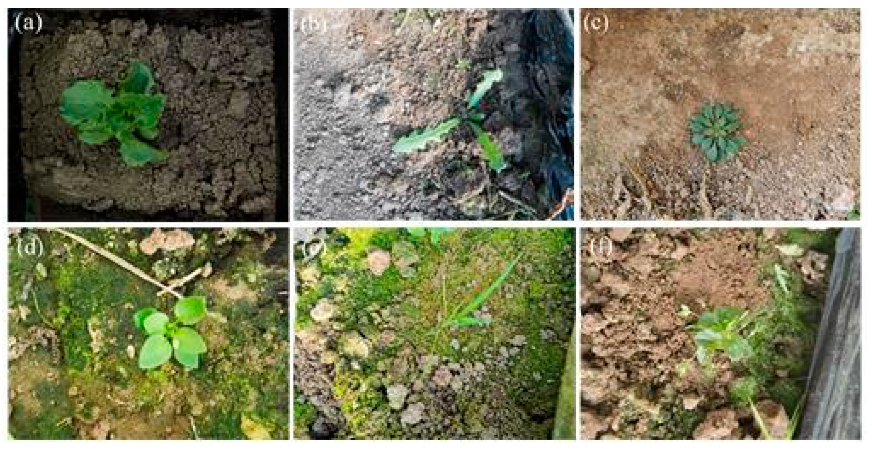
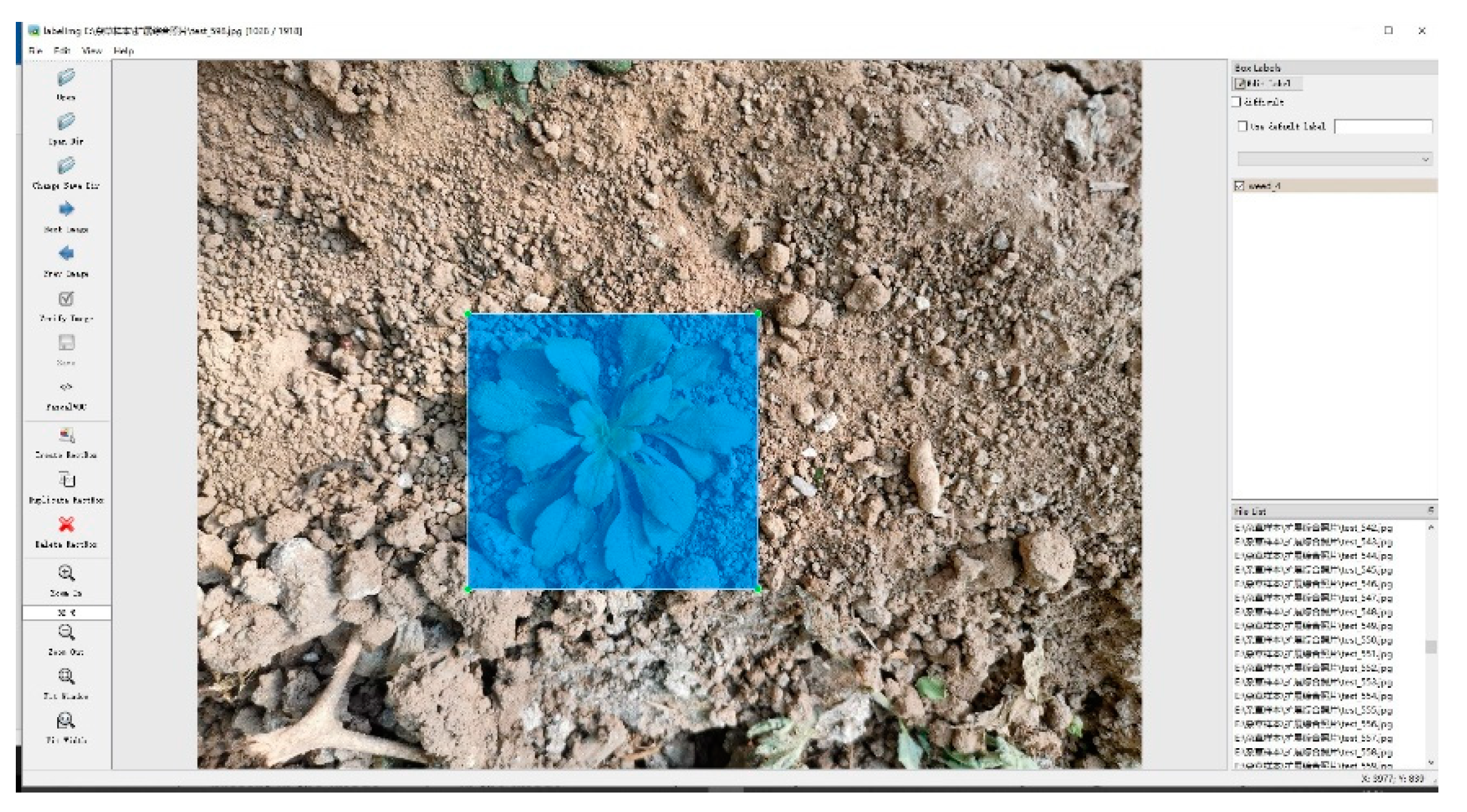
2.1. Dataset Preparation

The lettuce and weed images were collected in Weifang, Shandong, China. The original dataset comprises 275 lettuce images and weed images of five species including 52 Geminate Speedwell (GS) weeds, 51 Wild Oats (WO) weeds, 54 Malachium Aquaticum (MA) weeds, 87 Asiatic Plantain (AP) weeds, and 23 Sonchus Brachyotus (SB) weeds, as shown in Figure 1. Since machine learning requires sufficient data for model training, it is necessary to employ data augmentation methods to build robust models. The original images of weeds and lettuces in this study were enhanced in two ways, including chroma adjustment (values in the range of 0.5 to 0.7 were randomly selected) and brightness adjustment (values in the range of 0.5 to 0.7 were randomly selected). For lettuce plants, 100 lettuce images were randomly selected for data augmentation, and the remaining 175 lettuce images were used as the test set. After data augmentation, the new dataset included 312 GS images, 306 WO images, 324 MA images, 408 AP images, 138 SB images, and 430 lettuce images. Three quarters of the plant images were selected for training while one quarter of the images were used for testing. Then, the texture features of different plants in the training set were extracted based on the local binary pattern (LBP) algorithm [16]. As shown in Figure 2, plant texture features were used to train the SVM model for class identification of each plant. In addition, the plant images in the new dataset were labeled using bounding boxes for training of different deep learning models including SSD [17], faster-RCNN [18], and YOLOv5x. The annotation of all images was performed manually using an image-annotation software (LabelImg, https://github.com/tzutalin/labelImg, accessed on 30 October 2021). Image annotation consisted of two steps. In the first step, entire plants were annotated (Figure 3). The information (such as class label, position coordinates of the bounding box) for each bounding box annotation was saved in XML files. In the second step, the XML files were converted to TXT tags for training models.

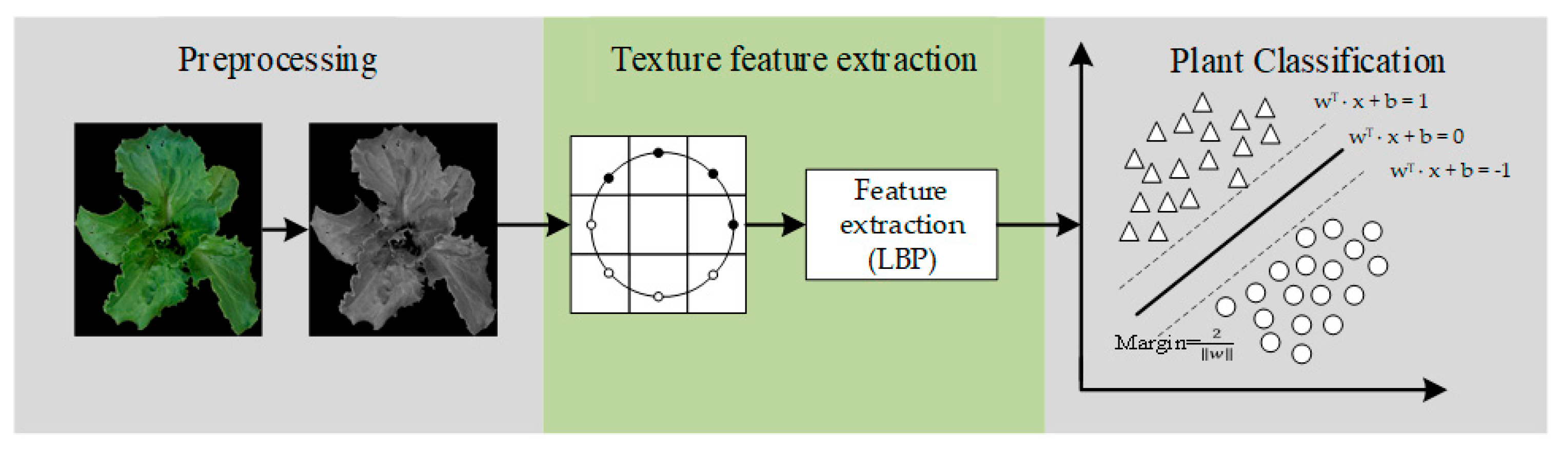
2.2. Texture Extraction

The rotation-invariant uniform local binary pattern ( L B P P , R r i u 2 ) algorithm, improved by Ojala et al. [19], was used to extract the feature vectors of the plants. The main characteristics of this algorithm are monotonic grayscale transformation, illumination, and rotation invariance. Compared with the original LBP algorithm, the improved L B P P , R r i u 2 algorithm can capture the crucial features. The L B P P , R r i u 2 can be expressed as follows:
L B P P , R r i u 2 = p = 0 P 1 s g p g c , if U L B P P , R 2 P + 1 , o t h e r w i s e ,
U L B P P , R = s g P 1 g c s g 0 g c + p = 1 P 1 s g p g c s g p 1 g c ,
where the g c express the gray value of the center pixel ( x c , y c ) . The g p are the sorted values, and p∈{0, 1, 2,...P−1}. In addition, P is the number of pixels in radius R. s is defined as
s ( x ) = 1 , x 0 0 , x < 0 .

2.3. Support Vector Machine (SVM)
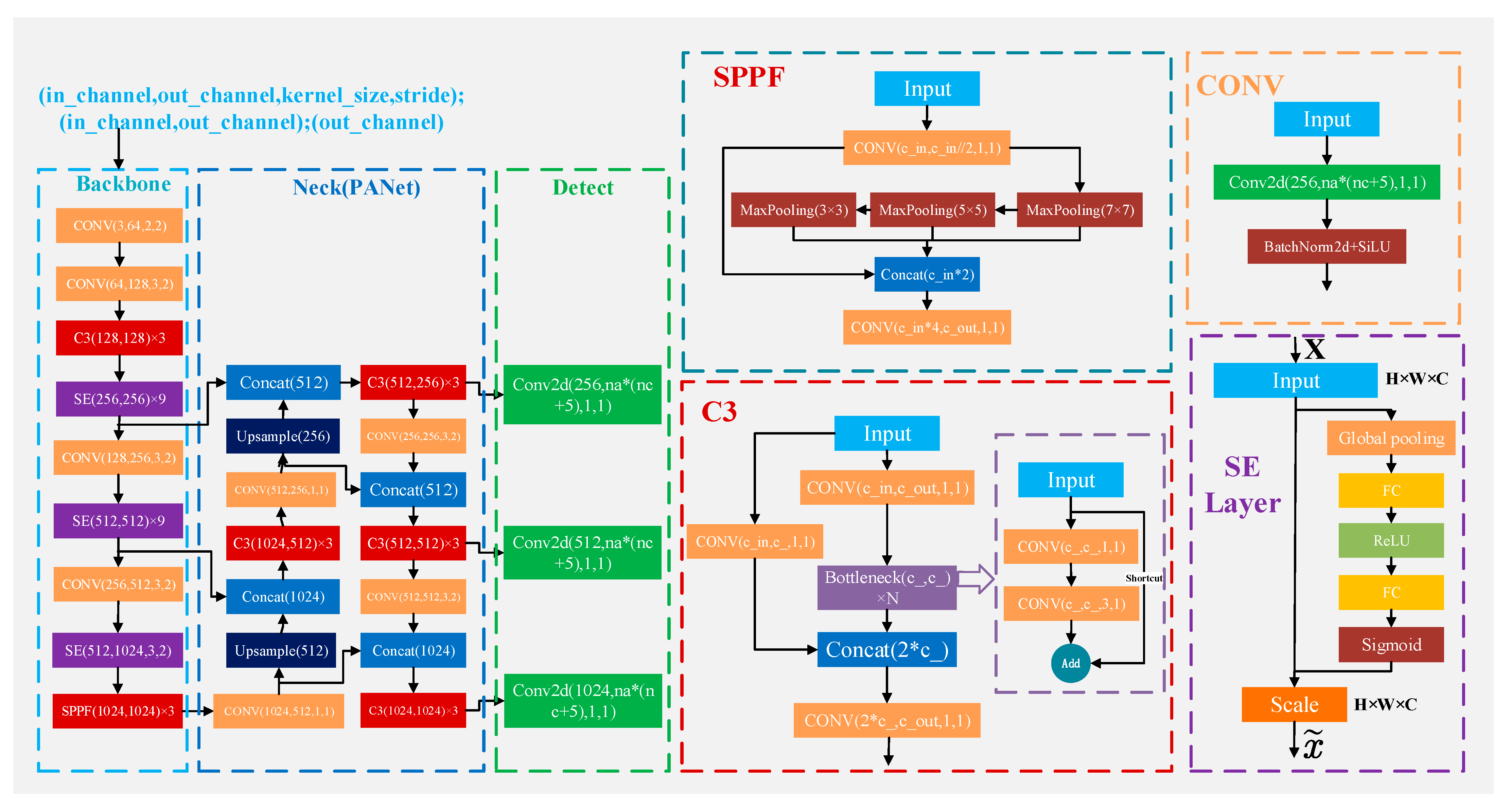
SVM was used for classification based on the following equation:
y ( x ) = w T x + b ,
where the parameters w and b are the weight and bias, respectively. They were calculated from the training dataset of feature vector x 1 ,…, x N with the corresponding target values t 1 , , t N , where ti∈{−1,1}. New data x is classified based on the sign of y(x). The SVM considers the margin concept to deal with the classification problem. The margin is defined as the smallest distance between the samples and the decision boundary.
The margin is calculated by the parameters w and b, as follows [20]:
arg max w , b 1 w min i t i w T x + b ,
To solve this calculated process, the Lagrange function is needed:
L ( w , b , a ) = 1 2 w 2 i = 1 N a i t i w T x + b 1 ,
where a is a vector of function whose element a i 0 . The element N is input data for training. The derivatives with respect to b and w are calculated to simplify Equation (6) as follows:
L ( w , b , a ) w = w i = 1 m a i y ( i ) x ( i ) = 0 ,
L ( w , b , a ) b = i = 1 m a i y ( i ) = 0 ,
Then, using these conditions, Equation (6) can be improved as follows:
L ˜ ( a ) = i = 1 N a i 1 2 i = 1 N j = 1 N a i a j t i t j K x i , x j ,
a i 0 , i = 1 , ... , N ,
i = 1 N a i t i = 0 ,
where K is a kernel function, which can transform the nonlinearly separable space to the linear separable one, and a i is the Lagrange multiplier.
The SVM was implemented using a computer (Intel® Core i7-6700HQ central process unit (CPU) @ 2.60 GHz, and 8 GB random-access memory (RAM)) with Python 3.8.0. The performance of the SVM in the plant classification was evaluated. After repeated experiments, we set the spatial and angular resolutions (P, R) of LBP operator values (8, 1). In this study, the linear kernel function was used to train the SVM model.

2.4. Deep Learning

2.4.1. Equipment

The hardware configurations were used for training and testing in this study on a computer (processor: Intel® Xeon® Platinum 8156 CPU; operating system: 64-bit Linux; memory: 24 GB). The training speed was improved in graphics processing unit (GPU) mode (NVIDIA GeForce RTX 3090). In order to avoid the influence of the hyperparameters on the experimental results, the hyperparameters of each network were configured uniformly. After repeated experiments, the hyperparameters were determined as follows: learning rate 0.001, epoch number 150, and batch size 16.

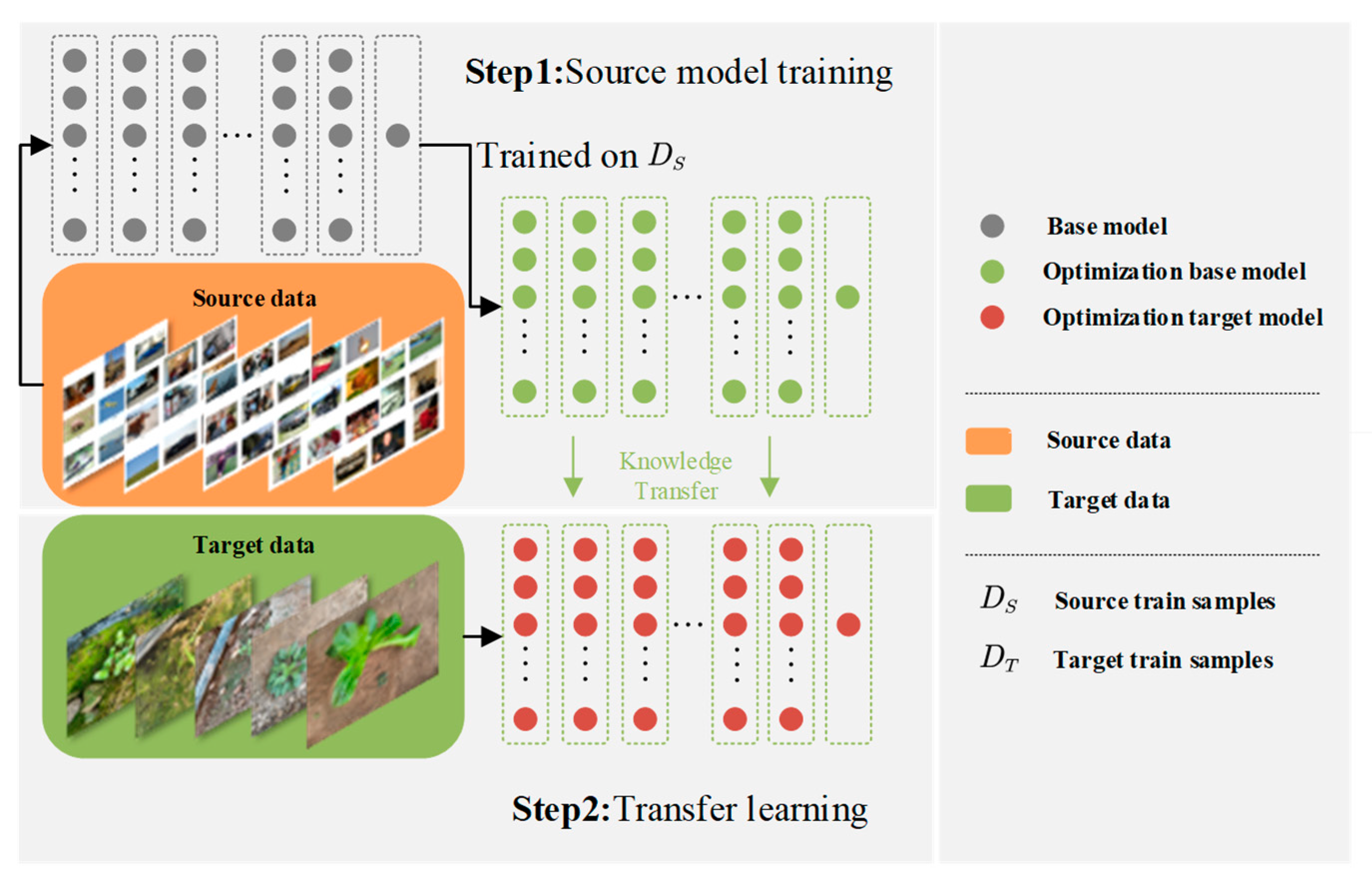
2.4.2. Transfer Learning
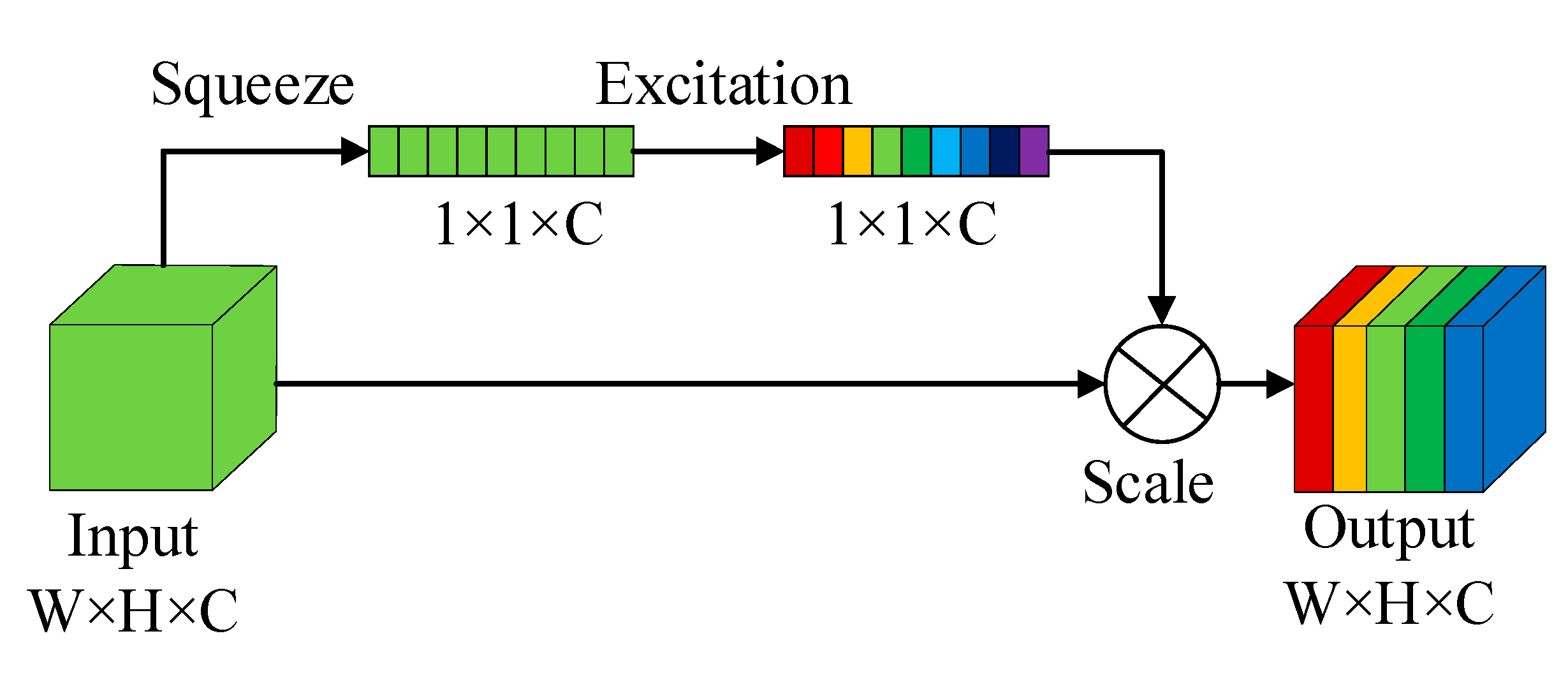
The transfer learning method was implemented by using pretrained weights (the pretraining weights were obtained by training the deep learning model in large-scale datasets). Transfer learning required characteristic extraction from pretrained weights. The output layer of the pretrained models is replaced by a fresh dense layer with the activation function. The fresh dense layer contains many nodes which were used to express the number of weeds and crops to be classified. Because the pretrained model was created, the time demanded for training a model using the transfer learning technique was shorter than when creating a new model from scratch [21]. Figure 4 shows the general workflow of the transfer learning method for training a deep learning model.

2.4.3. SE Network

In recent years, the attention mechanism technologies have been extensively used in the deep learning field [22]. Great progress has been made in employing attention mechanisms in the domains of image segmentation and natural language processing [23]. An attention mechanism concentrates attention on interesting or useful areas to eliminate unnecessary features. Then, it can distribute various weights to every feature for improving the accuracy and efficiency of the model [24]. SE is a typical channel attention mechanism that has the benefits of simple structure and convenient deployment. SE is primarily composed of three basic parts [25]:
(1) The basic content of F s q (squeeze operation) is global average pooling. In this way, global spatial information can be compressed into channel descriptors. A single two-dimensional feature channel is converted into a real number and makes it a global feature. The output one-dimensional matrix likes Z = [ z 1 , z 2 , ... , z c ] , where the c-th element of Z can be expressed as follows:
z c = F s q u c = 1 W × H i = 1 W j = 1 H u c ( i , j ) ,
where H and W are the height and width of the feature map of a single feature channel, respectively. u c ( i , j ) is the value of every point on the feature map channel.
(2) Next, the F e x (excitation operation) generates different weights to assign to each channel. Then, it establishes the dependencies between various channels. z is a one-dimensional matrix obtained by F s q . Both W 1 and W 2 are the full connection layers. F e x can be interpreted as follows:
s = F e x ( z , W ) = σ W 2 δ W 1 z ,
where δ   and   σ are the activation function ReLU and sigmoid.
(3) The F e x is applied to obtain the weight s of different channels and the output. After rescaling the transformation output y n , the block output is obtained. The F s c a l e (reweight operation) can be interpreted as follows:
x ˜ n = F s c a l e y n , s n = s n · y n ,
where s n is the weight value of the nth channel and y n is the two-dimension matrix of the output of the nth channel. In addition, x ˜ n is the output feature of the different channels after adding weight.
As shown in Figure 5, the SE network can obtain the global description of the input terminal through the squeeze operation. Then, the weight of each feature channel is obtained by the excitation operation and the key features are extracted. The SE-YOLOv5x model is developed by embedding the SE network into the YOLOv5x model. The reconstruction model is shown in Figure 6.

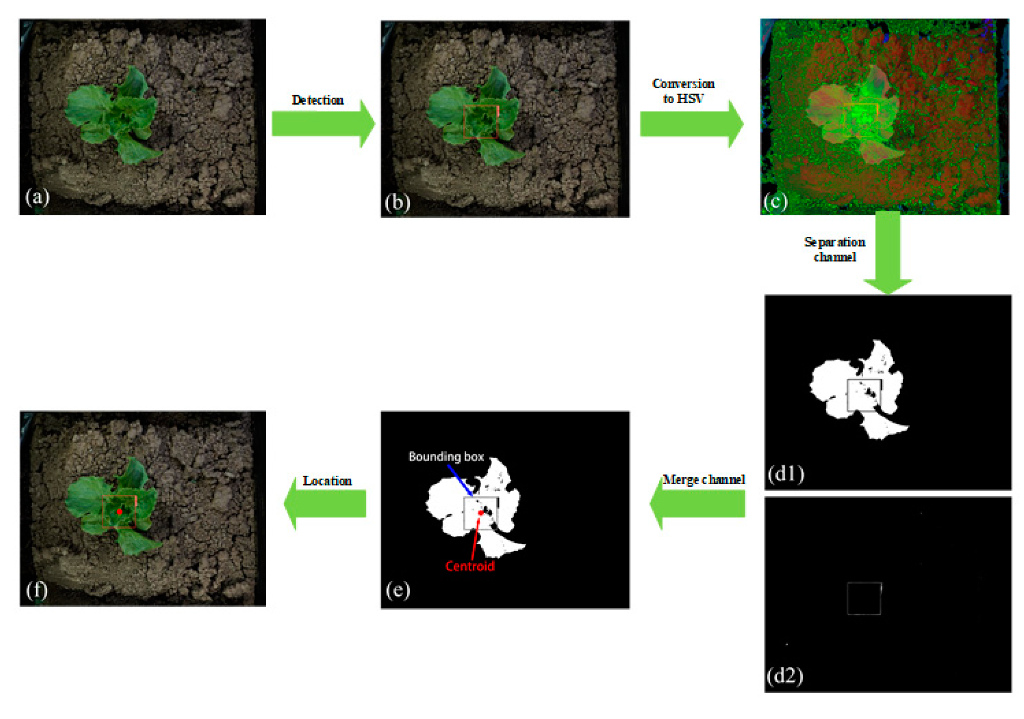
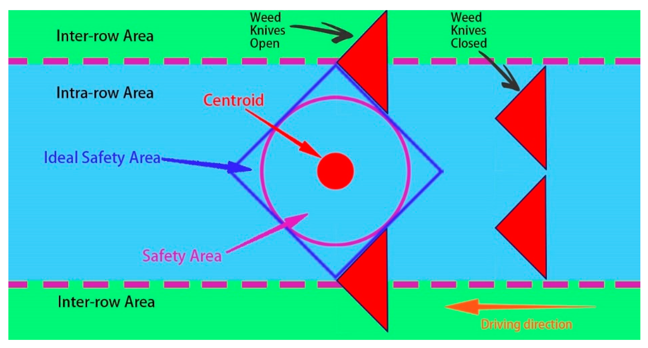
2.5. Localization of Lettuce Stem Emerging Point

The localization method was realized based on bounding box generated by the deep learning models and the hue, saturation, and value (HSV) color space. Specifically, lettuce that is anchored to a lone location exhibits an overall approximately radial symmetry. Based on this truth, the central position of the bounding box around the crop should be considered as the evaluated stem position in the image frame. The precision of the stem position is immediately proportional to how exactly the bounding box locates the weeds or crops. Thus, identifying the tender leaves proved to be more accurate than directly identifying the whole seedling when locating the crop center. The deep learning model was used to identify the tender leaves located in the center of the lettuce, as shown in Figure 7b. Then, image processing was used to extract the center coordinates. In addition, green leaf weeds can easily affect the extraction of lettuce coordinates due to the similar color of crops and weeds, during the process of extraction. The HSV color space is a choice for eliminating interference from the natural environment. Therefore, this research treated lettuce and bounding boxes separately in the HSV color space. The lettuce and bounding box can be segmented by transferring to the HSV color space and using the green and red channels separately. As shown in Figure 7c, the HSV color space was gained from the following formula:
H = 60 ( G B ) / ( V min ( R , G , B ) ) i f V = R 120 + 60 ( B R ) / ( V min ( R , G , B ) ) i f V = G 240 + 60 ( R G ) / ( V min ( R , G , B ) ) i f V = B ,
S = V min ( R , G , B ) V i f V 0 0 o t h e r w i s e ,
V = max ( R , G , B ) ,
if H < 0 then H = H + 360 . On output 0 V 1 , 0 S 1 , 0 H 360 . In the formula, R , G , B represent the values in the red, green, and blue color channels, respectively. Then, the red and green channels are separated by a mask covering in the HSV color space.
After the separation of color channels, the bounding box and lettuce were extracted. In this process, some of the other boxes and impurities were extracted too. The method of filling the connected domain was used to remove the interference of weed surrounding frames and impurities, as can be seen in Figure 7(d1,d2). The formulas for removing the connected domain are as follows:
g ( x , y ) = 255 , i f a r e a > S min 0 , o t h e r w i s e ,
y ( x , y ) = 255 , i f a r e a < S max 0 , o t h e r w i s e
In the formula, g ( x , y ) and y ( x , y ) are judgment functions of the bounding box and crop, respectively. area represents the actual area of each connected domain in the image. S min and S max are the minimum and maximum threshold, respectively.
The new lettuce and bounding box images were obtained after filtering out small connected areas. The images of the two channels were merged, as shown in Figure 7e. Finally, the lettuce stem center coordinates were located according to the bounding box and the morphological characteristics of lettuce, as shown in Figure 7f. The formulas are shown as follows:
X = x max + x min 2 ,
Y = y max + y min 2
In the formula, (X, Y) represents the coordinates of the positioned lettuce center. x max , x min , y max , and y min are the coordinates of the four corners of the rectangular bounding box surrounding the crop.
This centripetal localization method based on the bounding box of tender leaves can locate the practical central coordinate of lettuce. It has the potential to control the opening and closing of the weeding knives to realize the removal of intra-row weeds in the lettuce field. The conceptual method combining center localization and weeding knives is shown in Figure 8. The weeding knives created a safety zone during opening and closing, and the concept of this safety area was also mentioned by Perez-Ruiz et al. [26]. In addition, the lettuce stem is approximately considered to be cylindrical, so its top view is a circle. The center of the circle is the ideal center coordinate. It can be regarded as a successful prediction when the predicted center coordinate is located in the stem circle area.

2.6. Evaluation Indicators

As shown in Equations (22)–(26), detailed evaluation indicators are defined to evaluate the results of all the deep learning and SVM models used in this study. As the dataset used in this study is uneven and the number of images of each plant sample varies, F1-score is also used to assess the image classification performance of the deep learning model. F1-score is obtained by calculating recall, precision, true negative (TN), true positive (TP), false negative (FN), and false positive (FP). Mean average precision (mAP) is used to estimate the effect of the target detection model. In addition, the loss of the deep learning model is used to estimate the error between the prediction results of the model and the ground truths. The losses consist of three parameters: object loss (obj_loss), classification loss (cls_loss), and bounding box loss (box_loss).
R e c a l l = t p t p + f n ,
P r e c i s i o n = t p t p + f p = t p n ,
F 1 s c o r e = 2 × P r e c i s i o n × R e c a l l P r e c i s i o n + R e c a l l ,
m A P = n = 1 N A P ( n ) N ,
l o s s = b o x _ l o s s + o b j _ l o s s + c l s _ l o s s ,

3. Results

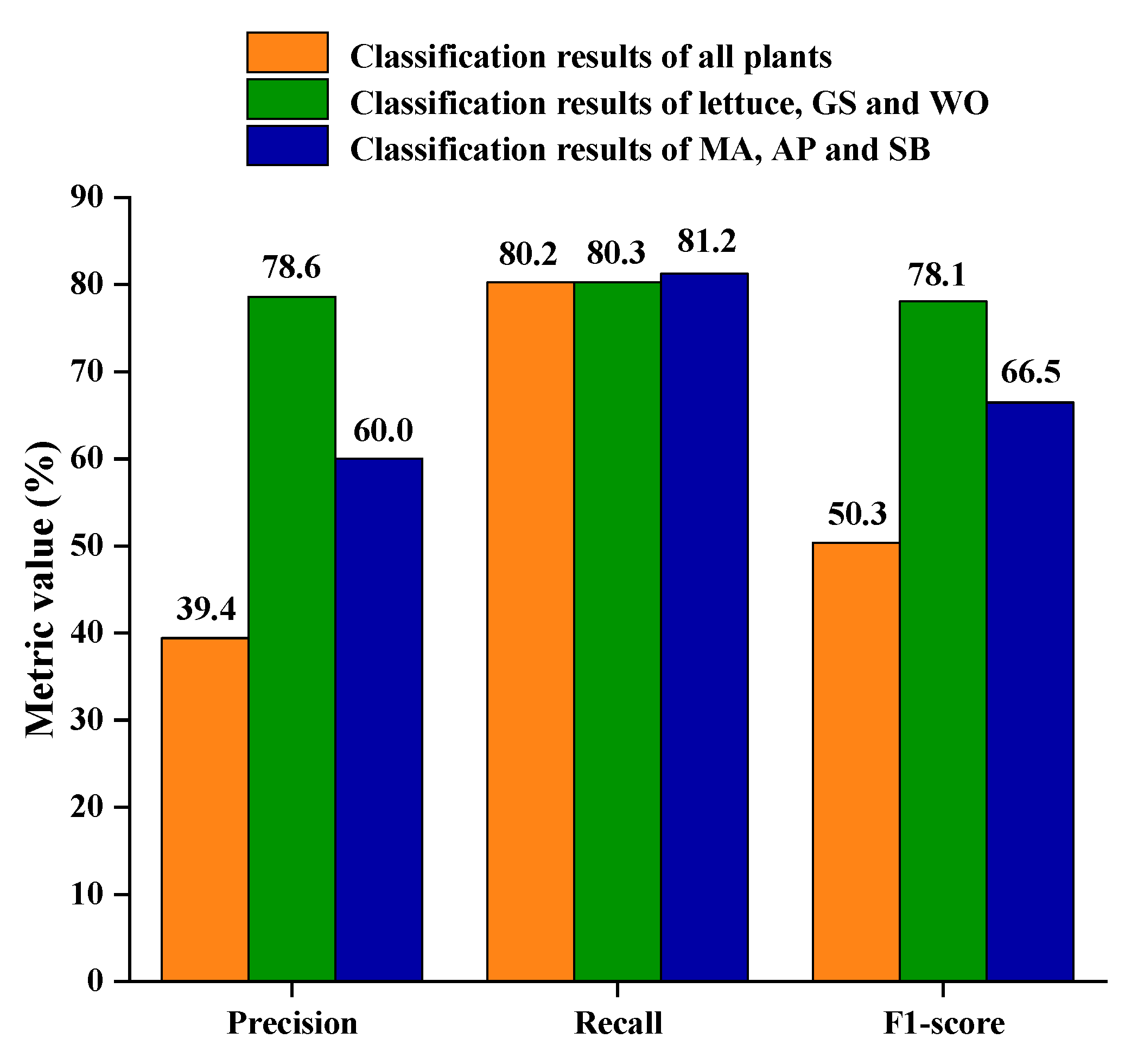
3.1. SVM for Plant Classification

The SVM model was established to identify different plants. Figure 9 shows the plant classification results based on SVM models developed with different datasets. When the SVM model was trained using the dataset containing six species of plants, the precision and F1-score of the SVM model were 39.4% and 50.3%. When the model was built using the data of three plants, the recall values of the SVM model were comparable but the precision and F1-score of the model increased substantially, regardless of whether the data contained lettuce crops or not. As can be seen, the precision and F1-score of the model containing the dataset of lettuce, GS, and WO were 78.6% and 78.1%, respectively. The precision and F1-score of the other model containing the dataset of MA, AP, and SB were 60.0% and 66.5%, respectively. The results showed that classification performance of SVM would become worse with the increase of plant species, which meant that the classical SVM was not qualified for multiclassification tasks.

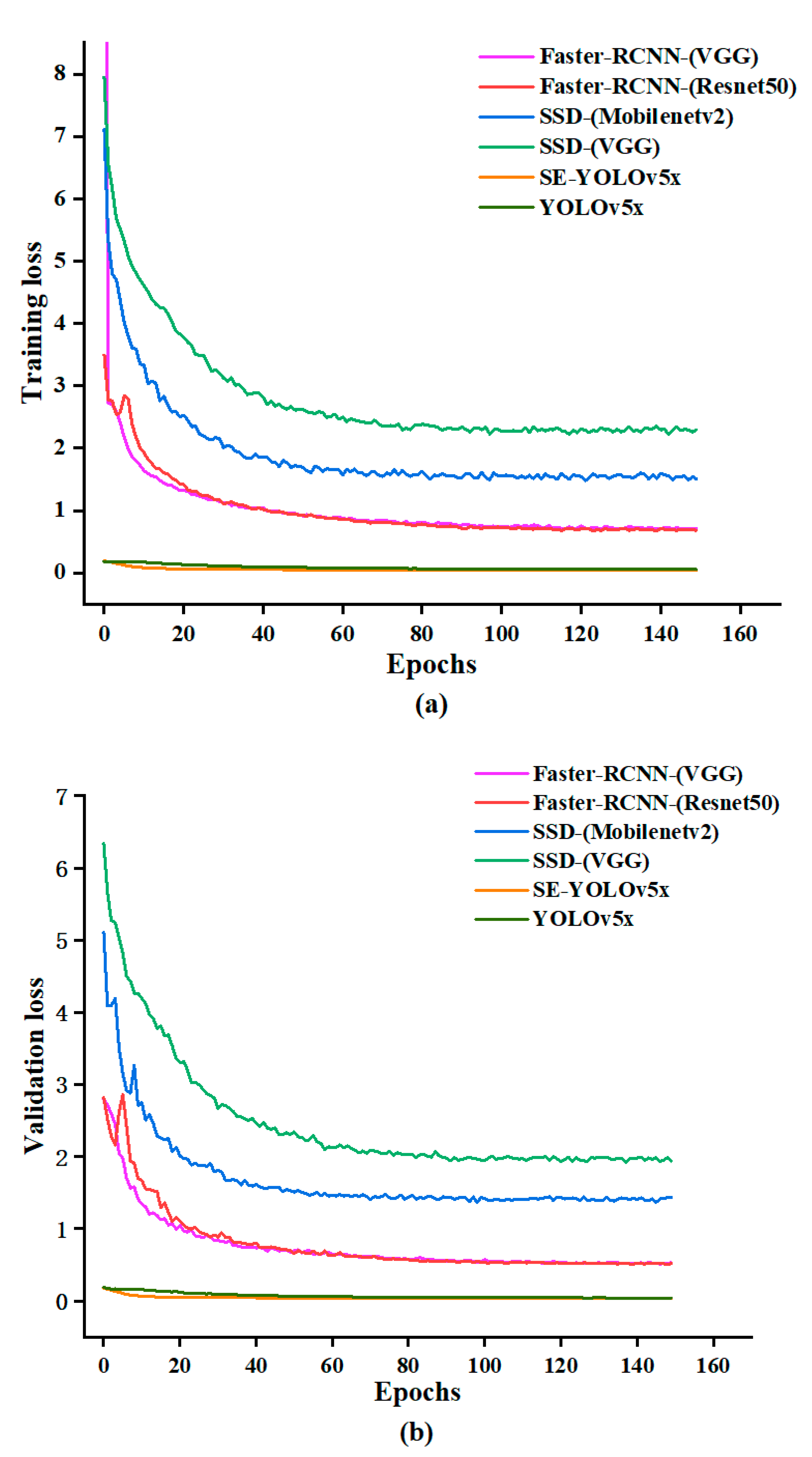
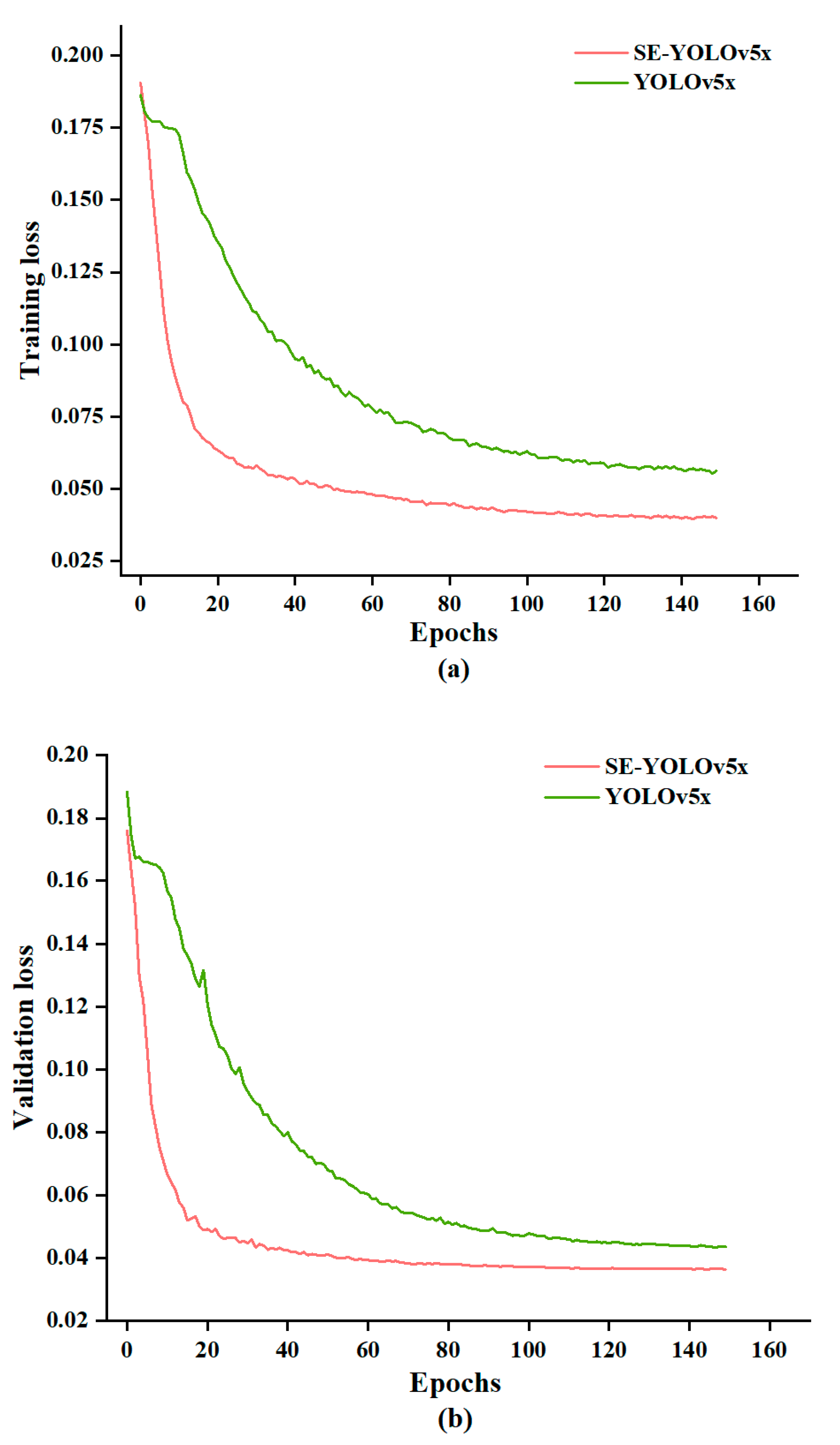
3.2. Training of Deep Learning Models

Figure 10a shows the variation curves of training loss with epochs in weed–lettuce identification. In general, the training loss curves of each model gradually tended to be stable with the increasing of epoch values. Specifically, the SE-YOLOv5x and YOLOv5x, compared with the other four models, were faster to converge and had lower loss value. In Figure 10, it was found that the SE-YOLOv5x and YOLOv5x gradually stabilized, and their training loss values were very close after 20 epochs. The training loss curves of faster-RCNN with two different backbones (VGG and Resnet50) were also very close, which gradually stabilized around the 40th epoch. The training loss of faster-RCNN with VGG backbone was slightly worse than that of faster-RCNN (Resnet50). SSD models with different backbones (VGG and Mobilenetv2) were stable around the 70th epoch. The SSD (VGG) had the highest training loss value after convergence.
The variation curves of validation loss with epochs of six models in identifying weeds and lettuce are shown in Figure 10b. Similar to training loss curves, the validation loss curves rapidly decreased in the early training stage (30 epochs) and then slowly converged at the end of training. As shown in Figure 10b, the SSD (VGG) model exhibited the highest loss value, and converged slowly after 60 epochs. The SSD (Mobilenetv2) had the fastest convergence rate and stabilized around the 50th epoch. Compared with the SSD model, the faster-RCNN (Resnet50) model had a lower initial loss and eventually achieved a lower loss value. The SE-YOLOv5x and YOLOv5x models exhibited the lowest loss values compared with the other four models. After the 20th epoch, the loss values of the improved SE-YOLOv5x and original YOLOv5x were very close and relatively stable. The main reason is that their accuracies are close to each other and higher than other models.
The corresponding loss curve changes of the SE-YOLOv5x and YOLOv5x were analyzed in detail, as shown in Figure 11. It was observed that the loss curves of both models gradually stabilized with the ever-increasing values of epochs. Specifically, the SE-YOLOv5x model converged the fastest, which gradually stabilized after 80 epochs. Figure 11 showed that each loss curve of the improved SE-YOLOv5x model decreased faster than the original YOLOv5x. The loss curves of the improved SE-YOLOv5x had a lower loss value. In conclusion, the improved SE-YOLOv5x model had better performance for the classification of lettuce and weeds compared with the original YOLOv5x model.

3.3. Deep Learning for Plant Classification

This research trained the object detection algorithms, including SE-YOLOv5x, YOLOv5x, faster-RCNN, and SSD. The backbone networks of some models were trained after being replaced by Mobilenetv2 [27] and Resnet50 [28]. The training results of these target detection algorithms are shown in Table 1. The precision, recall, mAP@0.5, and F1-score of the SE-YOLOv5x model were 0.976, 0.956, 0.971, and 0.973, respectively. The evaluation indicators of the SE-YOLOv5x model were the best of all the models. The results proved the effectiveness of the SE-YOLOv5x model in classifying weeds in lettuce field. In addition, the weight size of the improved SE-YOLOv5x was only 105.9 MB, reduced by 39.52% compared with the original YOLOv5x weight. The recognition speed was 19.1 ms, improved by 34.14%, compared with the original YOLOv5x. The SE-YOLOv5x model can enormously reduce the model size and increase the recognition speed while maintaining high recognition accuracy due to using the SE network. For some embedded mobile devices, their RAM space is limited and calculating power is not enough, and cannot satisfy large-scale and high-intensity operations. Therefore, the SE-YOLOv5x is suitable for embedded mobile devices.
As shown in Table 2, the classification performance of SE-YOLOv5x in identifying individual plant species was further investigated. The classification results of the SE-YOLOv5x model show the precision, recall, and F1-score for each weed species and the lettuce crop. The highest F1-score was 99.8% for lettuce, and the lowest F1-score was 90.0% for MA. The precision of GS, WO, MA, AP, SB, and lettuce were 100%, 98%, 89.8%, 98.7%, 99.5%, and 99.6%, respectively. For identification of MA, the precision value was not high, and was only less than 90%, but the model for the rest of the plants reached a significantly high accuracy. In summary, the SE-YOLOv5x model had a strong capability in classification of weeds and lettuce plants.

3.4. Performance Comparison of SVM and Deep Learning Models

In this part, a comparison is presented between the classic SVM model and six deep learning models. The SVM and deep learning models were trained based on the dataset including six plants. The SVM was trained with L B P 8 , 1 r i u 2 /256 × 256/C = 1. Table 3 shows the modeling results of SVM and deep learning methods. It can be observed that the mean performance of the deep learning models outperformed the SVM method. Except for recall value, the performance of the SVM was the worst among all these models. Moreover, it could be observed that the classification effect of the SSD models with different backbones (VGG and Mobilenetv2) was better than that of the faster-RCNN models with different backbones (VGG and Resnet50), although the recall of the SSD models was lower than that of the faster-RCNN models. Due to using the SE network, the SE-YOLOv5x model achieved the highest accuracies, with precision, recall, and F1-score of 97.6%, 95.6%, and 97.3%, respectively. The F1-score of the SE-YOLOv5x surpassed the SVM by 47%. The SE-YOLOv5x model showed very excellent results in identifying weeds and lettuce. In conclusion, deep learning models performed better than the classical SVM method in multiclassification, and the SE-YOLOv5x model performed the best among all deep learning models.

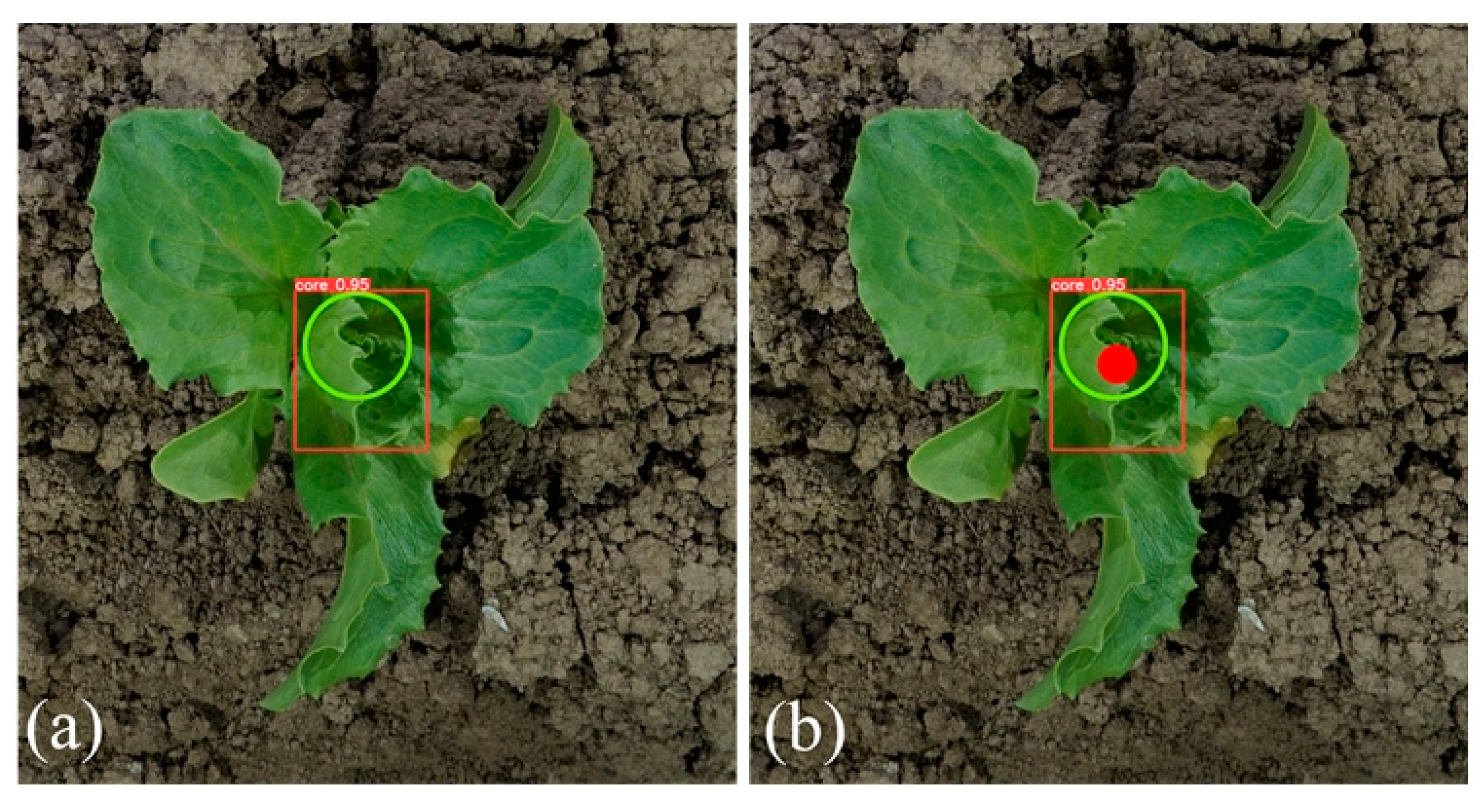
3.5. Determination of Lettuce Stem Emerging Point

Table 4 shows the testing results of different deep learning models in lettuce stem emerging point localization. The average diameter of lettuce stem at the stage of 4–6 leaves was about 20 mm. As the tender leaves of lettuce grew from the middle of the lettuce rhizome, the area of the lettuce stem was marked using green circles in the lettuce image shown in Figure 12. Compared with the original YOLOv5x, faster-RCNN (Resnet50 and VGG), and SSD (Mobilenetv2 and VGG) models, the SE-YOLOv5x model located the lettuce stem emerging point more accurately with the accuracy of 97.14%. When different backbone networks (such as Resnet50, VGG in faster-RCNN or Mobilenetv2, and VGG in SSD models) were considered, it was found that the VGG backbone networks achieved higher accuracy than others. Even though the faster-RCNN model was superior to the SSD model in weeds and lettuce classification, it was inferior to the SSD model in lettuce stem emerging point localization. There were two main reasons for the decline of localization accuracy: firstly, the recognition accuracy of the deep learning model itself has an important influence on localization results. In addition, the growth of the edge leaves is more irregular, which also increases the difficulty of locating the lettuce stem emerging point. Therefore, the SE-YOLOv5x model was adopted for locating the stem emerging points of lettuce.

4. Discussion

In this study, an optimized SE-YOLOv5x method was developed for weed-crop classification and localization of lettuce stem emerging point in a complex background. The performance of different deep learning models (such as improved SE-YOLOv5x, original YOLOv5x, SSD with VGG or Mobilenetv2 backbone, and faster-RCNN with Resnet50 or VGG backbone) were compared for classification of weeds and lettuce plants. Then, a unique method was proposed for localization of lettuce stem emerging points based on the bounding box location. The training results showed that the SE-YOLOv5x model was the best in weed-crop classification and plant localization in a lettuce field. In the future, more weed species should be considered. Moreover, the data annotation is extraordinarily laborious and time-consuming. Thus, automatic labeling should be realized by advanced annotation methods. In addition, equipment should be developed for real-time image acquisition under the variable natural environmental conditions (such as sunlight and wind) that occur in the crop field. In this study, only the network framework of YOLOv5x was considered for object detection. Other YOLOv5 algorithms (such as YOLOv5s, YOLOv5m, and YOLOv5l) should be considered in the future. Although the YOLOv5 network has four versions (YOLOv5s, v5m, v5l, v5x), YOLOv5x achieved the best performance compared to the other models in public datasets.
The SE-YOLOv5x model yielded an F1-score as high as 97.14%, and a test time of a single image of 19.1 ms. Table 5 shows the related research results on plant identification based on CNN in recent years. Specifically, Wang et al. [29] proposed a DeepSolanum-Net model to identify solanum rostratum dunal plants. The model achieved an F1-score of 0.901 with a test time of 131.88 ms. Zou et al. [30] developed a modified U-Net to segment the green bristlegrass in complex background, with an F1-score of 0.936 and a test time of 51.71 ms. Although the above studies performed well in segmenting the plants, the F1-scores and test times were lower than the proposed method in the current study. Jin et al. [31] combined the Centernet and image processing for identifying bok choy and Chinese white cabbage with a test time of 8.38 ms, but its F1-score was only 0.953. Garibaldi-Marquez et al. [20] designed a vision system to classify three species of plants (Zea mays, narrow-leaf weeds, and broadleaf weeds) using the VGG16 model. The F1-score (97.7%) of VGG16 was higher than that of the SE-YOLOv5x in the current study, but its test time was much longer (194.56 ms). In addition, in the study of Veeranampalayam Sivakumar et al. [32], object detection-based faster-RCNN models were used over low-altitude unmanned aerial vehicle (UAV) imagery for weed detection in soybean fields, yielding an F1-score of just 66.0% and a test time of 230 ms. Although Chen et al. [33] reported an accuracy (F1-score = 98.93 ± 0.34%) for recognition of 15 weed classes in cotton fields that was similar to our study (F1-score = 97.3%), their test time (338.5 ± 0.1 ms) for detection was very long. As shown in Table 4, the test times of the methods proposed by Wang et al. [34] and Jin et al. [35] are shorter than that of the SE-YOLOv5x, but their F1-scores are lower. The results of this research show that the improved SE-YOLOv5x model has great potential for weed-crop classification and localization. However, this study is an initial work. Further research should be conducted to develop a ground-based automated four-wheel-driving robot equipped with knives to remove the weeds. The ideal vehicle should be lightweight, low-cost, and robust enough to conduct automatic weed removal and deal with various abnormal situations [36,37,38,39,40].

5. Conclusions

In this study, the SE-YOLOv5x model was used for weed-crop classification and lettuce localization. The model was optimized by attention mechanism and transfer learning. Compared with the classical SVM method and other deep learning models (such as SSD and faster-RCNN) with different backbones (such as VGG, Resnet50, and Mobilenetv2), the optimized SE-YOLOv5x model exhibited the highest precision, recall, mAP@0.5, and F1-score values of 97.6%, 95.6%, 97.1%, and 97.3% in weed-crop classification, respectively. The accuracy of localization of lettuce stem emerging points based on the SE-YOLOv5x model was 97.14%. The knowledge generated by this research will greatly facilitate the efficient identification and removal of weeds in fields.

Author Contributions

Conceptualization, W.-H.S.; methodology, J.-L.Z.; software, J.-L.Z.; validation, J.-L.Z.; formal analysis, J.-L.Z.; investigation, J.-L.Z.; resources, W.-H.S.; writing—original draft preparation, J.-L.Z.; writing—review and editing, W.-H.S., H.-Y.Z. and Y.P.; supervision, W.-H.S.; project administration, W.-H.S.; funding acquisition, W.-H.S. All authors have read and agreed to the published version of the manuscript.

Funding

This research was funded by National Natural Science Foundation of China, grant number 32101610.

Data Availability Statement

Data are available on request due to privacy.

Conflicts of Interest

The authors declare no conflict of interest.

References

  1. Gao, J.; Nuyttens, D.; Lootens, P.; He, Y.; Pieters, J.G. Recognising weeds in a maize crop using a random forest machine-learning algorithm and near-infrared snapshot mosaic hyperspectral imagery. Biosyst. Eng. 2018, 170, 39–50. [Google Scholar] [CrossRef]
  2. Pérez-Ruiz, M.; Slaughter, D.C.; Gliever, C.J.; Upadhyaya, S.K. Automatic GPS-based intra-row weed knife control system for transplanted row crops. Comput. Electron. Agric. 2012, 80, 41–49. [Google Scholar] [CrossRef]
  3. Tang, J.; Wang, D.; Zhang, Z.; He, L.; Xin, J.; Xu, Y. Weed identification based on K-means feature learning combined with convolutional neural network. Comput. Electron. Agric. 2017, 135, 63–70. [Google Scholar] [CrossRef]
  4. Ahmed, F.; Al-Mamun, H.A.; Bari, A.S.M.H.; Hossain, E.; Kwan, P. Classification of crops and weeds from digital images: A support vector machine approach. Crop Prot. 2012, 40, 98–104. [Google Scholar] [CrossRef]
  5. Ferreira, A.D.; Freitas, D.M.; da Silva, G.G.; Pistori, H.; Folhes, M.T. Weed detection in soybean crops using ConvNets. Comput. Electron. Agric. 2017, 143, 314–324. [Google Scholar] [CrossRef]
  6. Ahmad, A.; Saraswat, D.; Aggarwal, V.; Etienne, A.; Hancock, B. Performance of deep learning models for classifying and detecting common weeds in corn and soybean production systems. Comput. Electron. Agric. 2021, 184, 106081. [Google Scholar] [CrossRef]
  7. Jiang, H.H.; Zhang, C.Y.; Qiao, Y.L.; Zhang, Z.; Zhang, W.J.; Song, C.Q. CNN feature based graph convolutional network for weed and crop recognition in smart farming. Comput. Electron. Agric. 2020, 174, 105450. [Google Scholar] [CrossRef]
  8. Osorio, K.; Puerto, A.; Pedraza, C.; Jamaica, D.; Rodríguez, L.J.A. A deep learning approach for weed detection in lettuce crops using multispectral images. AgriEngineering 2020, 2, 471–488. [Google Scholar] [CrossRef]
  9. Hu, K.; Coleman, G.; Zeng, S.; Wang, Z.; Walsh, M. Graph weeds net: A graph-based deep learning method for weed recognition. Comput. Electron. Agric. 2020, 174, 105520. [Google Scholar] [CrossRef]
  10. Abdalla, A.; Cen, H.; Wan, L.; Rashid, R.; Weng, H.; Zhou, W.; He, Y. Fine-tuning convolutional neural network with transfer learning for semantic segmentation of ground-level oilseed rape images in a field with high weed pressure. Comput. Electron. Agric. 2019, 167, 105091. [Google Scholar] [CrossRef]
  11. Picon, A.; San-Emeterio, M.G.; Bereciartua-Perez, A.; Klukas, C.; Eggers, T.; Navarra-Mestre, R. Deep learning-based segmentation of multiple species of weeds and corn crop using synthetic and real image datasets. Comput. Electron. Agric. 2022, 194, 106719. [Google Scholar] [CrossRef]
  12. Wang, Z.P.; Jin, L.Y.; Wang, S.; Xu, H.R. Apple stem/calyx real-time recognition using YOLO-v5 algorithm for fruit automatic loading system. Postharvest Biol. Technol. 2022, 185, 111808. [Google Scholar] [CrossRef]
  13. Zhang, D.-Y.; Luo, H.-S.; Wang, D.-Y.; Zhou, X.-G.; Li, W.-F.; Gu, C.-Y.; Zhang, G.; He, F.-M. Assessment of the levels of damage caused by Fusarium head blight in wheat using an improved YoloV5 method. Comput. Electron. Agric. 2022, 198, 107086. [Google Scholar] [CrossRef]
  14. Gong, H.; Mu, T.; Li, Q.; Dai, H.; Li, C.; He, Z.; Wang, W.; Han, F.; Tuniyazi, A.; Li, H.; et al. Swin-Transformer-Enabled YOLOv5 with Attention Mechanism for Small Object Detection on Satellite Images. Remote Sens. 2022, 14, 2861. [Google Scholar] [CrossRef]
  15. Hu, J.; Shen, L.; Albanie, S.; Sun, G.; Wu, E. Squeeze-and-Excitation Networks. IEEE Trans. Pattern Anal. Mach. Intell. 2020, 42, 2011–2023. [Google Scholar] [CrossRef]
  16. Le, V.N.T.; Apopei, B.; Alameh, K. Effective plant discrimination based on the combination of local binary pattern operators and multiclass support vector machine methods. Inf. Processing Agric. 2019, 6, 116–131. [Google Scholar]
  17. Liu, W.; Anguelov, D.; Erhan, D.; Szegedy, C.; Reed, S.; Fu, C.-Y.; Berg, A.C.; Detector, S.S.D.S.S.M.; Leibe, I.B.; Matas, J.; et al. (Eds.) Computer Vision—ECCV 2016; Springer International Publishing: Cham, Switzerland, 2016; pp. 21–37. [Google Scholar]
  18. Ren, S.Q.; He, K.M.; Girshick, R.; Sun, J. Faster R-CNN: Towards Real-Time Object Detection with Region Proposal Networks. In Proceedings of the 29th Annual Conference on Neural Information Processing Systems (NIPS), Montreal, Canada, 11–12 December 2015. [Google Scholar]
  19. Ojala, T.; Pietikainen, M.; Maenpaa, T. Multiresolution gray-scale and rotation invariant texture classification with local binary patterns. IEEE Trans. Pattern Anal. Mach. Intell. 2002, 24, 971–987. [Google Scholar] [CrossRef]
  20. Garibaldi-Marquez, F.; Flores, G.; Mercado-Ravell, D.A.; Ramirez-Pedraza, A.; Valentin-Coronado, L.M. Weed Classification from Natural Corn Field-Multi-Plant Images Based on Shallow and Deep Learning. Sensors 2022, 22, 3021. [Google Scholar] [CrossRef]
  21. Christopher, M.; Beighith, A.; Bowd, C.; Proudfoot, J.A.; Goldbaum, M.H.; Weinreb, R.N.; Girkin, C.A.; Liebmann, J.M.; Zangwill, L.M. Performance of Deep Learning Architectures and Transfer Learning for Detecting Glaucomatous Optic Neuropathy in Fundus Photographs. Sci. Rep. 2018, 8, 16685. [Google Scholar] [CrossRef]
  22. Qi, J. An improved YOLOv5 model based on visual attention mechanism: Application to recognition of tomato virus disease. Comput. Electron. Agric. 2022, 194, 106780. [Google Scholar] [CrossRef]
  23. Chen, J.; Zhang, D.; Zeb, A.; Nanehkaran, Y.A. Identification of rice plant diseases using lightweight attention networks. Expert Syst. Appl. 2021, 169, 114514. [Google Scholar] [CrossRef]
  24. Zhu, X.; Cheng, D.; Zhang, Z.; Lin, S.; Dai, J. An Empirical Study of Spatial Attention Mechanisms in Deep Networks. In Proceedings of the 2019 IEEE/CVF International Conference on Computer Vision (ICCV), Seoul, Korea, 27 October–2 November 2019; pp. 6687–6696. [Google Scholar]
  25. Hu, J.; Shen, L.; Sun, G. Squeeze-and-excitation networks. In Proceedings of the IEEE Conference on Computer Vision and Pattern Recognition, Salt Lake City, UT, USA, 18–23 June 2018; pp. 7132–7141. [Google Scholar]
  26. Perez-Ruiz, M.; Slaughter, D.C.; Fathallah, F.A.; Gliever, C.J.; Miller, B.J. Co-robotic intra-row weed control system. Biosyst. Eng. 2014, 126, 45–55. [Google Scholar] [CrossRef]
  27. Sandler, M.; Howard, A.; Zhu, M.L.; Zhmoginov, A.; Chen, L.C. MobileNetV2: Inverted Residuals and Linear Bottlenecks. In Proceedings of the 31st IEEE/CVF Conference on Computer Vision and Pattern Recognition (CVPR), Salt Lake City, UT, USA, 18–23 June 2018; pp. 4510–4520. [Google Scholar]
  28. Wang, F.; Jiang, M.; Qian, C.; Yang, S.; Li, C.; Zhang, H.; Wang, X.; Tang, X. Residual Attention Network for Image Classification. In Proceedings of the 2017 IEEE Conference on Computer Vision and Pattern Recognition (CVPR), Honolulu, HI, USA, 21–26 July 2017; pp. 6450–6458. [Google Scholar]
  29. Wang, Q.; Cheng, M.; Xiao, X.; Yuan, H.; Zhu, J.; Fan, C.; Zhang, J. An image segmentation method based on deep learning for damage assessment of the invasive weed Solanum rostratum Dunal. Comput. Electron. Agric. 2021, 188, 106320. [Google Scholar] [CrossRef]
  30. Zou, K.; Chen, X.; Wang, Y.; Zhang, C.; Zhang, F. A modified U-Net with a specific data argumentation method for semantic segmentation of weed images in the field. Comput. Electron. Agric. 2021, 187, 106242. [Google Scholar] [CrossRef]
  31. Jin, X.; Che, J.; Chen, Y. Weed Identification Using Deep Learning and Image Processing in Vegetable Plantation. IEEE Access 2021, 9, 10940–10950. [Google Scholar] [CrossRef]
  32. Sivakumar, A.N.V.; Li, J.; Scott, S.; Psota, E.; Jhala, A.J.; Luck, J.D.; Shi, Y. Comparison of Object Detection and Patch-Based Classification Deep Learning Models on Mid- to Late-Season Weed Detection in UAV Imagery. Remote Sens. 2020, 12, 2136. [Google Scholar] [CrossRef]
  33. Chen, D.; Lu, Y.; Li, Z.; Young, S. Performance evaluation of deep transfer learning on multi-class identification of common weed species in cotton production systems. Comput. Electron. Agric. 2022, 198, 107091. [Google Scholar] [CrossRef]
  34. Wang, Q.; Cheng, M.; Huang, S.; Cai, Z.; Zhang, J.; Yuan, H. A deep learning approach incorporating YOLO v5 and attention mechanisms for field real-time detection of the invasive weed Solanum rostratum Dunal seedlings. Comput. Electron. Agric. 2022, 199, 107194. [Google Scholar] [CrossRef]
  35. Jin, X.; Sun, Y.; Che, J.; Bagavathiannan, M.; Yu, J.; Chen, Y. A novel deep learning-based method for detection of weeds in vegetables. Pest Manag. Sci. 2022, 78, 1861–1869. [Google Scholar]
  36. Su, W.-H. Advanced Machine Learning in Point Spectroscopy, RGB- and Hyperspectral-Imaging for Automatic Discriminations of Crops and Weeds: A Review. Smart Cities 2020, 3, 767–792. [Google Scholar] [CrossRef]
  37. Su, W.-H.; Fennimore, S.A.; Slaughter, D.C. Fluorescence imaging for rapid monitoring of translocation behaviour of systemic markers in snap beans for automated crop/weed discrimination. Biosyst. Eng. 2019, 186, 156–167. [Google Scholar] [CrossRef]
  38. Su, W.-H.; Fennimore, S.A.; Slaughter, D.C. Development of a systemic crop signalling system for automated real-time plant care in vegetable crops. Biosyst. Eng. 2020, 193, 62–74. [Google Scholar]
  39. Su, W.-H.; Slaughter, D.C.; Fennimore, S.A. Non-destructive evaluation of photostability of crop signaling compounds and dose effects on celery vigor for precision plant identification using computer vision. Comput. Electron. Agric. 2020, 168, 105155. [Google Scholar] [CrossRef]
  40. Su, W.-H. Crop plant signalling for real-time plant identification in smart farm: A systematic review and new concept in artificial intelligence for automated weed control. Artif. Intelli. Agric. 2020, 4, 262–271. [Google Scholar]
Figure 1. Examples of lettuce and weed images. (a) An example of lettuce, (b) an example of Sonchus Brachyotus (SB), (c) an example of Asiatic Plantain (AP), (d) an example of Malachium Aquaticum (MA), (e) an example of Wild Oats (WO), and (f) an example of Geminate Speedwell (GS).
Agronomy 12 02061 g001
Figure 2. General scheme of the classification method based on support vector machine (SVM).
Agronomy 12 02061 g002
Figure 3. Bounding box annotation of an AP.
Agronomy 12 02061 g003
Figure 4. The process of transfer learning.
Agronomy 12 02061 g004
Figure 5. The structure of the squeeze-and-excitation (SE) network.
Agronomy 12 02061 g005
Figure 6. The structure of the SE-YOLOv5x model.
Agronomy 12 02061 g006
Figure 7. The visualization process of center positioning algorithm; (a) the original image captured, (b) the detection result of the deep learning model, (c) the color space image of HSV (the image of detection result is converted from RGB to HSV channel by image processing), (d1,d2) the separation results of crop and bounding box in different channels, (e) the result of merging color channel, (f) the final localization result.
Agronomy 12 02061 g007
Figure 8. The working process of the weeding knives: on the right side of the figure, the weed knives were placed in the closed position where they are close to each other, and they can kill all weeds in the intra-row area. In the center of this figure, the weed knives were placed in the open position in order to bypass the lettuce plant.
Agronomy 12 02061 g008
Figure 9. Comparison of SVM modeling results using different datasets.
Agronomy 12 02061 g009
Figure 10. (a) Training loss curves and (b) validation loss curves against the number of epochs in weed–lettuce classification.
Agronomy 12 02061 g010
Figure 11. (a) The training loss curves and (b) the validation loss curves of SE-YOLOv5x and YOLOv5x.
Agronomy 12 02061 g011
Figure 12. (a) The SE-YOLOv5x identification results of the tender leaves; (b) localization results.
Agronomy 12 02061 g012
Table 1. Lettuce and weeds classification results of different deep learning models.
ModelPrecision (%)Recall (%)mAP@0.5% (%)F1-Score (%)
SE-YOLOv5x97.695.697.197.3
YOLOv5x96.795.096.295.8
SSD (VGG)89.477.286.280.7
SSD (Mobilenetv2)94.887.195.190.6
Faster-RCNN (Resnet50)54.089.081.565.7
Faster-RCNN (VGG)50.588.983.862.8
Table 2. Classification results of different plants based on SE-YOLOv5x model on PyTorch.
Plant SpeciesPrecision (%)Recall (%)mAP@0.5 (%)F1-Score (%)
GS 1100.098.399.599.1
WO 298.088.692.093.1
MA 389.890.292.790.0
AP 498.799.199.498.9
SB 599.597.699.398.5
Lettuce99.6100.099.599.8
1 Geminate Speedwell; 2 Wild Oats; 3 Malachium Aquaticum; 4 Asiatic Plantain; 5 Sonchus Brachyotus.
Table 3. Training results of the SVM and different deep learning models for crop/weed identification.
ModelPrecision (%)Recall (%)F1-Score (%)
SE-YOLOv5x97.695.697.3
YOLOv5x96.795.095.8
SSD (VGG)89.477.280.7
SSD (Mobilenetv2)94.887.190.6
Faster-RCNN (Resnet50)54.089.065.7
Faster-RCNN (VGG)50.588.962.8
SVM39.480.250.3
Table 4. Test results of different deep learning models in lettuce stem emerging point localization.
ModelTotal SamplesThe Number of Detected SamplesAccuracy (%)
Faster-RCNN (Resnet50)17514080.00
Faster-RCNN (VGG)17515286.86
SSD (Mobilenetv2)17512169.14
SSD (VGG)17512470.86
YOLOv5x17516896.00
SE-YOLOv5x17517097.14
Table 5. A summary of plant identification based on different CNN models.
ReferenceModelPlantF1-Score (%)Test Time (ms)
Wang et al. [29]DeepSolanum-NetSolanum rostratum dunal90.1131.88
Zou et al. [30]Modified U-NetGreen bristlegrass93.651.71
Jin et al. [31]Centernet + image processingBok choy and Chinese white cabbage (various growth stages)95.38.38
Garibaldi-Marquez et al. [20]VGG16 + ROI detection algorithmsZea mays, narrow-leaf weeds, and broadleaf weeds97.7194.56
Veeranampalayam Sivakumar et al. [32]Faster-RCNNWaterhemp, Palmer amaranthus, common lambsquarters, velvetleaf, foxtail species66.0230.00
Wang et al. [34]YOLO-CBAMSolanum rostratum dunal seedlings92.410.51
Chen et al. [33]ResNeXtMorning glory, Carpetweed, Palmer amaranth, Waterhemp, Purslane, and so on98.93 ± 0.34338.5 ± 0.1
Jin et al. [35]YOLOv3 + image processingBok choy97.118.0
Proposed methodSE-YOLOv5xGS, WO, MA, AP, SB, lettuce97.319.1
Publisher’s Note: MDPI stays neutral with regard to jurisdictional claims in published maps and institutional affiliations.

