Article

Climatic Mechanism of Delaying the Start and Advancing the End of the Growing Season of Stipa krylovii in a Semi-Arid Region from 1985–2018

1
Department of Atmospheric and Oceanic Sciences & Institute of Atmospheric Sciences, Fudan University, Shanghai 200438, China
2
State Key Laboratory of Severe Weather, Chinese Academy of Meteorological Sciences, Beijing 100081, China
3
Joint Eco-Meteorological Laboratory of Chinese Academy of Meteorological Sciences and Zhengzhou University, Zhengzhou 450001, China
4
College of Resources and Environmental Sciences, China Agricultural University, Beijing 100193, China
*
Author to whom correspondence should be addressed.
Agronomy 2022, 12(8), 1906; https://doi.org/10.3390/agronomy12081906
Submission received: 22 July 2022 / Revised: 10 August 2022 / Accepted: 12 August 2022 / Published: 14 August 2022

Abstract

:
Plant phenological variations depend largely on temperature, but they cannot be explained by temperature alone in arid and semi-arid regions. To reveal the response mechanisms of grassland phenology to climate change, the effects of temperature, moisture and light at the start (SOS), peak (POS) and end (EOS) of the growing season for Stipa krylovii (S. krylovii) in Inner Mongolian grassland was analysed from 1985–2018 with partial least squares (PLS) regression. The results showed that the SOS was significantly delayed at a rate of 5.4 d/10a (change over 10 years), while POS and EOS were insignificantly advanced, which were inconsistent with the existing understanding that climate warming advances the SOS and delays the EOS. The vapor pressure deficit (VPD) in July, maximum air temperature (Tmax) in September of the previous year, diurnal temperature range (DTR) from mid-February to mid-March, and Tmax from late March to mid-April of the current year were the critical factors and periods triggering the SOS, which contributed to 68.5% of the variation in the SOS. Additionally, the minimum air temperature (Tmin) occurred from mid-December to late December, and precipitation (PRE) occurred from mid-June to late July for POS, which could explain 52.1% of POS variations. In addition, Tmax from late August to early September influenced the EOS with an explanation of 49.3%. The results indicated that the phenological variations in S. krylovii were the result of the combined effects of climatic conditions from the previous year and the current year. Additionally, an increase in the preseason DTR delayed the SOS, and excessive summer precipitation induced an earlier POS, while warming in early autumn induced an earlier EOS, reflecting the adaptation mechanism of the perennial dense-cluster herbaceous plants in semi-arid regions to climate change. These findings could enrich the understanding of plant phenology in response to climate change.

1. Introduction

Grassland ecosystems are highly sensitive and vulnerable to regional and even global climate change [1,2]. Plant phenology is a composite indicator of the sensitivity of ecosystem processes to climate change [1]. The start of the growing season (SOS), peak of the growing season (POS) and end of the growing season (EOS) of grassland plants indicate the beginning, maximum and ending periods of photosynthesis, respectively [3,4]. Therefore, the SOS, POS and EOS of grasslands play an important role in the carbon cycle of terrestrial ecosystems [5,6]. Revealing the changes in SOS, POS and EOS and their response to climate change are of great significance for diagnosing the adaptation of ecosystems to regional climate change and predicting carbon exchange in regional ecosystems [7,8,9,10].
In recent decades, an advanced SOS and delayed EOS of plants have been widely reported due to global warming in the Northern Hemisphere [11,12,13]. In addition, the POS exhibited advancing (–6.8 d/10 a) (change over 10 year) and delaying (2.9 d/10 a) trends in temperate and alpine grasslands, respectively [14]. However, the direction and magnitude of grassland phenology in arid and semi-arid regions showed large spatial variability [4,15,16]. Additionally, the interannual variations in plant phenology were also large enough [17]. A delayed SOS was observed for many grassland species [18]. Different climatic drivers of the phenology in different areas might have driven the increased interannual variability [19].
A growing number of studies have shown that temperature and precipitation are the two major influential controls on the spatial variation in grassland phenology [2,11,20]. For example, Tao et al. [11] suggested that the increase in temperature promoted an earlier SOS, while the relationship between SOS and precipitation varied among vegetation types. The SOS would be advanced by 1–6 days with an increase in temperature of 1 °C in Inner Mongolia, Qinghai-Tibetan Plateau [21]. In addition, a higher preseason temperature induced a significantly earlier SOS and later EOS, while preseason precipitation had a weak effect on the SOS and EOS [4]. Guo et al. [22] revealed that higher temperatures promoted typical grassland plants to green-up in relatively humid regions in Inner Mongolia, and the effect of precipitation was more important in regions limited by water availability [23,24]. In contrast to the above results, during the optimum length period, a 10 mm increase in autumn precipitation may lead to a delay of 0.2–4 days in the EOS, and a 1 °C increase in the mean autumn minimum temperature may induce a delay of 1.6–9.3 days in the EOS across the alpine grasslands [25]. Liu et al. [26] and Wang et al. [27] noted that the performance of phenology models that consider only temperature and light is poor, and they suggested incorporating precipitation as an additional predictor in phenology models. Heat requirement-based phenology models have also been shown to have large uncertainty when predicting ecosystem carbon and water balance responses to climate variability [28].
The relationship between phenology and climatic factors in grassland can vary significantly during a specific period. Many studies have identified the effect of climatic factors on plant phenology on a monthly scale [29,30], even though this time scale may be too coarse. Climate variations during some critical periods are thought to have a greater regulatory effect on plant phenology [31]. Ren et al. [32] emphasized that there are obvious time windows for temperature and precipitation to effect grassland phenology, and the performance of the phenology models depends largely on the predefined preseason length used to quantify the predictor variables [27]. Therefore, accurately defining and assessing the differences in the effects of climatic factors with higher temporal resolution on plant phenology may improve the accuracy of plant phenology models [33,34].
Partial least squares (PLS) regression has been used to recognize plant phenological responses to daily scale climatic factors [35,36,37,38]. However, previous studies mainly used mean temperature to identify phenology when using PLS regression [36,39]. In addition, few studies have tried to detect the response of grassland phenology to other climatic factors [40]. Little is known about the effects of daily scale precipitation and light on the phenology of grassland plants [31], which limits the improvement of the accuracy of grassland phenology models. In addition, long-term phenological observations at the species-level and at specific sites can provide direct evidence for the effects of climate change [41]. However, there is little evidence from long-term in situ observations of the effects of climate warming on grassland phenology [16].
Therefore, a full consideration of potential climate drivers and further analysis of the response of grassland phenology to climate change based on updated long-term plant phenology data are urgently needed. We hypothesize that precipitation plays an important role in semi-arid regions and there are significant time window differences in the phenology response to temperature, precipitation and sunshine hours in S. krylovii. The objectives of this study were: (1) to analyse the long-term variation in SOS, POS and EOS for Stipa krylovii (S. krylovii) in semi-arid region; (2) to reveal the critical periods of potential climatic factors driving the phenology of S. krylovii; and (3) to determine to what extent these potential climatic factors can explain the phenological variations in S. krylovii.

2. Materials and Methods

2.1. Study Area and Data

The study area is located in the middle of the Inner Mongolian Autonomous Region (116°19′ E, 44°08′ N) in China, which is a typical temperate semi-arid continental climate zone. The mean annual temperature and mean annual precipitation were 3.2 °C and 273 mm from 1982–2019, respectively [27]. S. krylovii and Leymus chinensis are two typical dominant species in this region [31,42]. In this study, S. krylovii is used as the species of focus. The phenology and meteorological data were obtained from the Xilinhot National Climate Observatory, Inner Mongolian, China Meteorological Administration. All meteorological data were examined and verified by the National Meteorological Information Center of the China Meteorological Administration.
The SOS, POS and EOS data for S. krylovii were obtained using phenological observation standards [43]. The size of the study area is 100 m × 100 m, which is fenced. It is divided into four equal experimental plots of 50 m × 50 m as four replicates. Each replicate is further divided into four observation areas, one of which is used for experiments in one year, with a cycle of four years. The species-specific phenological observations are carried out for ten individual herbaceous plants every 2 days by professionals according to uniform observation criteria [44]. SOS, POS and EOS are evaluated as follows: (1) when 50% of individual herbaceous plants display green leaves that grow up to one centimetre in spring, the period is identified as the SOS; (2) when 50% of individual herbaceous plants in the plot show spikes from the top or lateral end of the leaf sheath, the stage represents the POS; (3) when 50% of individual herbaceous plants in the plot turn yellow (approximately two-thirds of the plant turns yellow), the period was judged to be the EOS. Julian days were used to indicate the SOS, POS and EOS on a particular day of the year (DOY).
Daily meteorological data from 1985–2018 were grouped into three classes: (1) temperature factors, including daily minimum air temperature (Tmin, °C), mean air (Tmean, °C) and maximum air temperature (Tmax, °C), and daily soil surface temperature (Tsoil, °C); (2) moisture factors, including daily precipitation (PRE, mm), vapor pressure deficit (VPD, kPa) and relative humidity (RH, %); and (3) light factor, including sunshine hours (SSH). The DTR describes the difference between the daily maximum and minimum temperatures as shown in Equation (1), which can represent diurnally asymmetric warming [45]. VPD describes the difference between the saturated water vapor pressure and the actual water vapor pressure, and the increase in this index inhibits the growth of vegetation [46]. VPD is estimated from RH and Tmean as shown in Equation (2) [47,48]. Based on the above data and previous research progress, this study focused on the impact of temperature factors (Tmean, Tmax, Tmin, Tsoil and DTR), moisture factors (PRE, RH and VPD) and light factor (SSH) on phenological variations.
D T R = T max T min
V P D = 0.611 × e 17.27 × T m e a n T m e a n + 237.3 × ( 1 R H 100 )
In Equation (1), Tmax and Tmin represent daily maximum and minimum air temperature, respectively. In Equation (2), Tmean (°C) indicates daily mean air temperature; RH (%) indicates relative humidity.

2.2. Identifying Critical Periods of Climatic Factors Driving Phenology

The partial least squares (PLS) regression was used to identify the critical periods when the phenology of S. krylovii had a strong response to variation in daily climatic factors during all 365 days of the year, based on data for 1985–2018. PLS, as a commonly used multivariate analysis method, is reliable for dealing with situations where independent variables are highly auto-correlated or where the number of independent variables exceeds the number of dependent variables [33,40]. The situations are encountered in relating variation of plant phenology to climatic factors at high temporal resolution [49].
The variable importance in the projection (VIP) and the standardized model coefficients (MC) are the two main output indices [33,36,50]. The VIP values were used to determine the explanatory ability of independent variables on dependent variables, with a higher VIP value (VIP ≥ 0.8) representing significant explanatory ability [51]. The MC values indicated a positive or negative effect of the independent variable on the dependent variable (MC > 0 indicated a delayed effect of climatic factors on the phenological period, and MC < 0 indicated an advanced effect of climatic factors on the phenological period). The VIP and MC values were output at a daily scale. The critical periods were determined with VIP greater than 0.8 and high absolute MC. To determine the critical periods, the SOS, POS and EOS were set as the dependent variables, and the daily temperature factors (Tmean, Tmax, Tmin, Tsoil and DTR), moisture factors (PRE, RH and VPD) and light factor (SSH) (all subjected to 31-day running mean) were set as the independent variables.
Furthermore, as a multiple linear regression method, stepwise linear regression reduces multicollinearity among climatic factors by selecting the combination of independent variables that are most suitable for the prediction of dependent variables [25]. Based on the PLS analysis, we developed stepwise linear regression models between climatic factors and phenology during the critical periods, to select the most suitable combination of independent variables (p < 0.05 by t test). All statistical analyses were performed with R programming language (R Core Team, 2022). The PLS was carried out using the ‘pls’ package.

3. Results

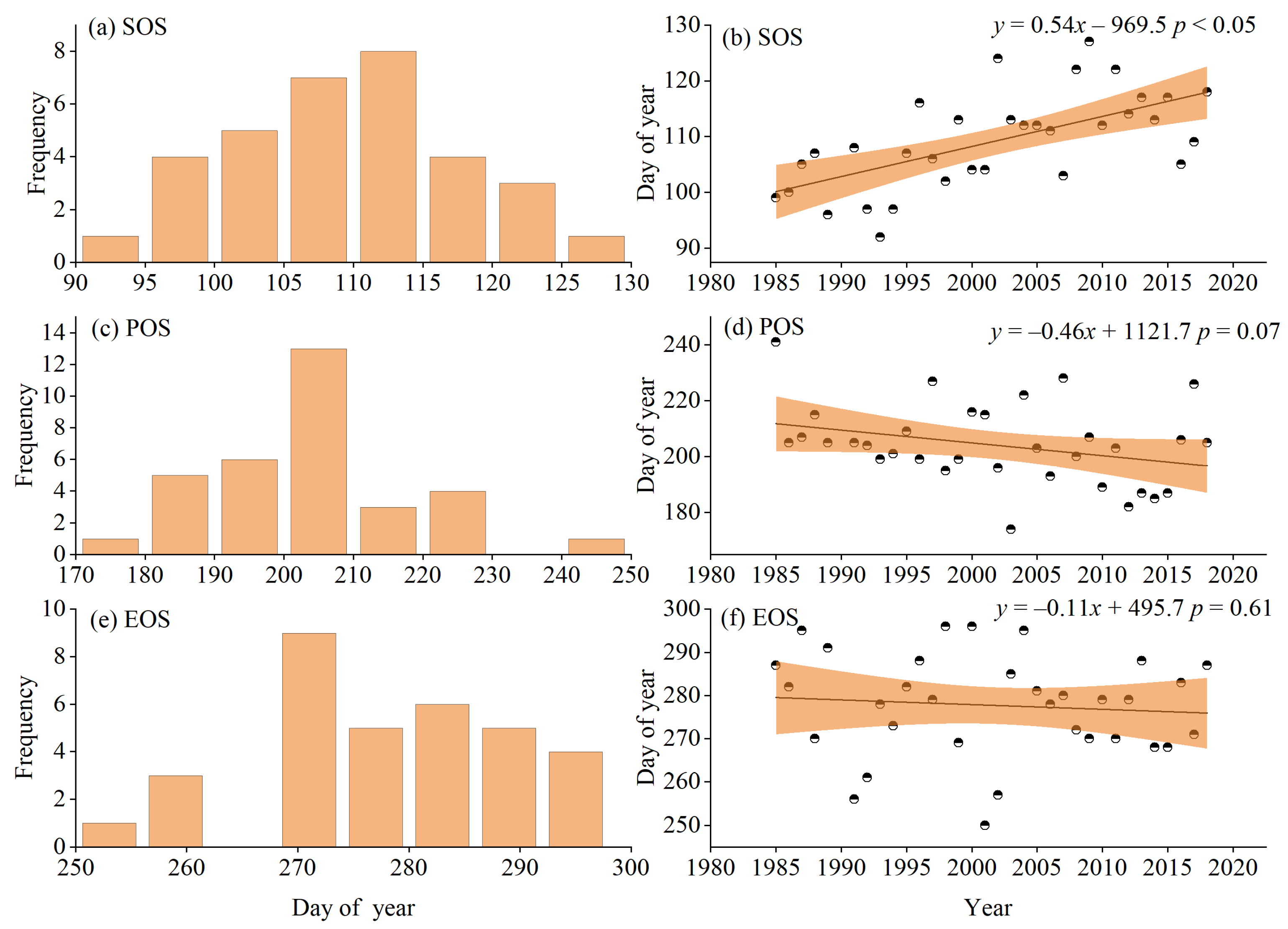
3.1. Phenological Change Characteristics from 1985–2018

The dynamic trend of SOS was significantly different, while POS and EOS were not (Figure 1). In detail, the SOS was mainly distributed over 105–115 days of the year, occurring on average in mid- to late April (Figure 1a), with a significantly delayed rate of 5.4 d/10 a (p < 0.05) (Figure 1b). The POS was mainly distributed over 200–210 days of the year, occurring on average in late July (Figure 1c). The POS was not significantly advanced (p > 0.05), even with a rate of 4.6 d/10 a (Figure 1d). Compared with the SOS and POS, the EOS showed greater variability and a slower rate of 1.1 d/10a (Figure 1e,f). In general, the SOS was notably delayed, while the POS and EOS did not advance significantly from 1985–2018.

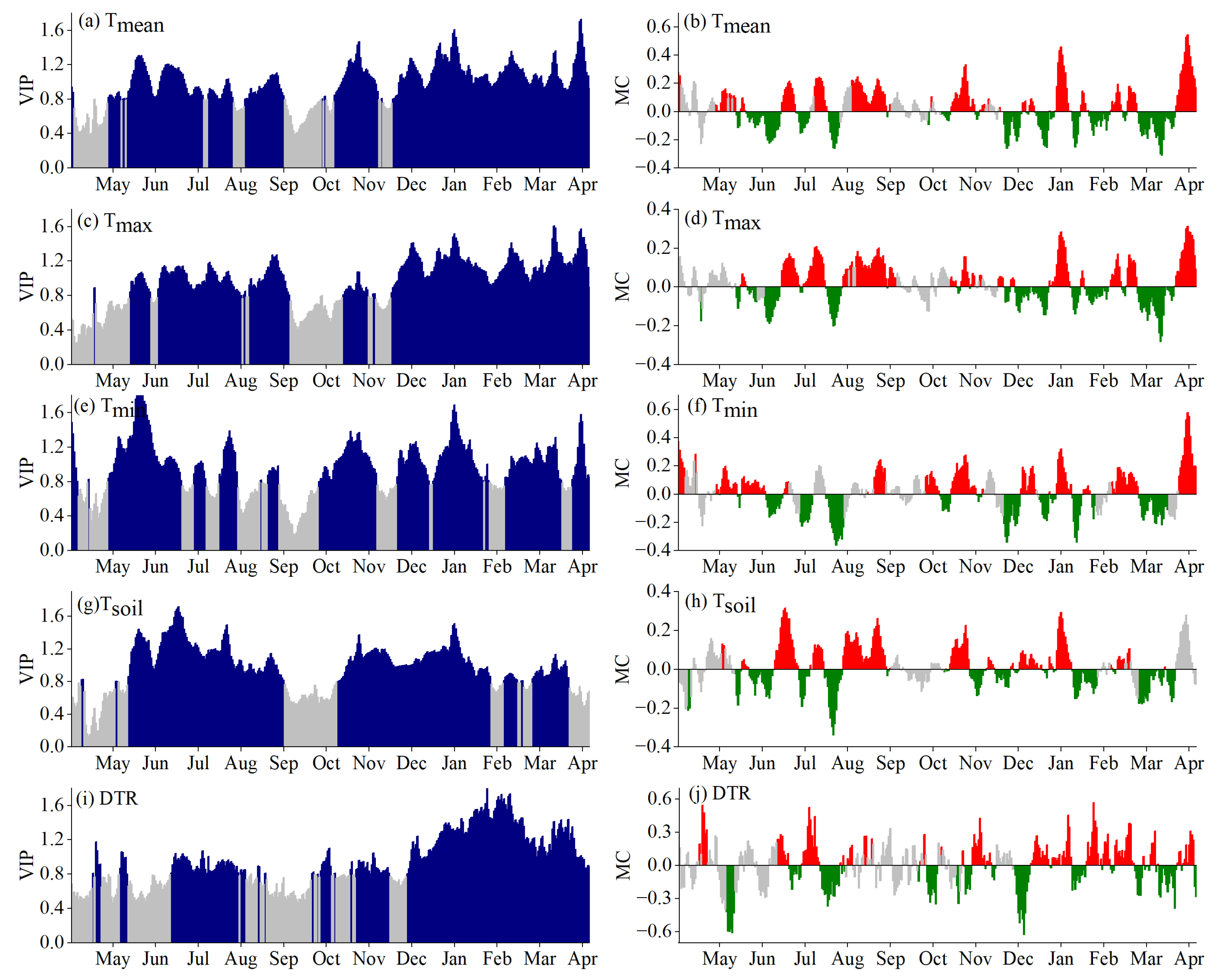
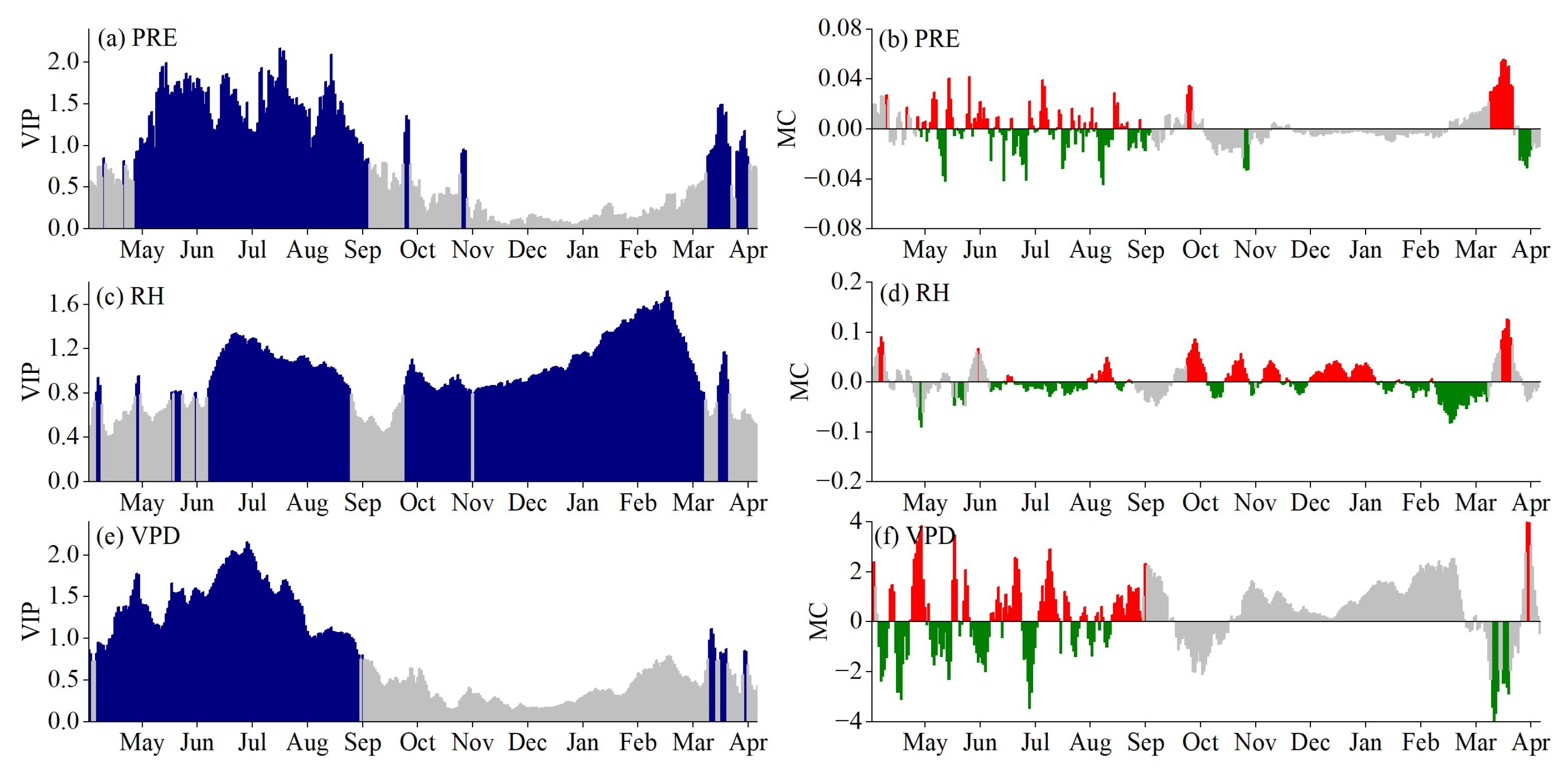
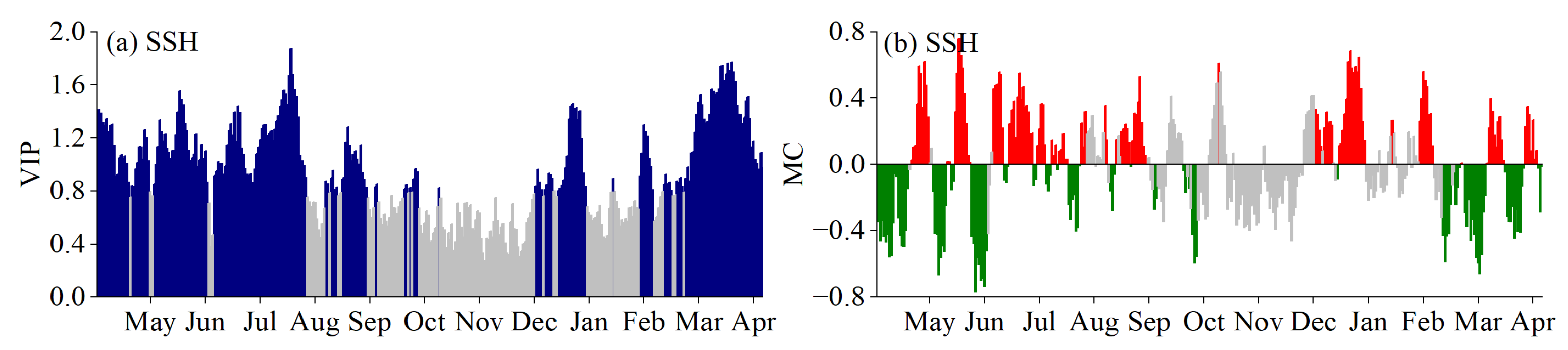
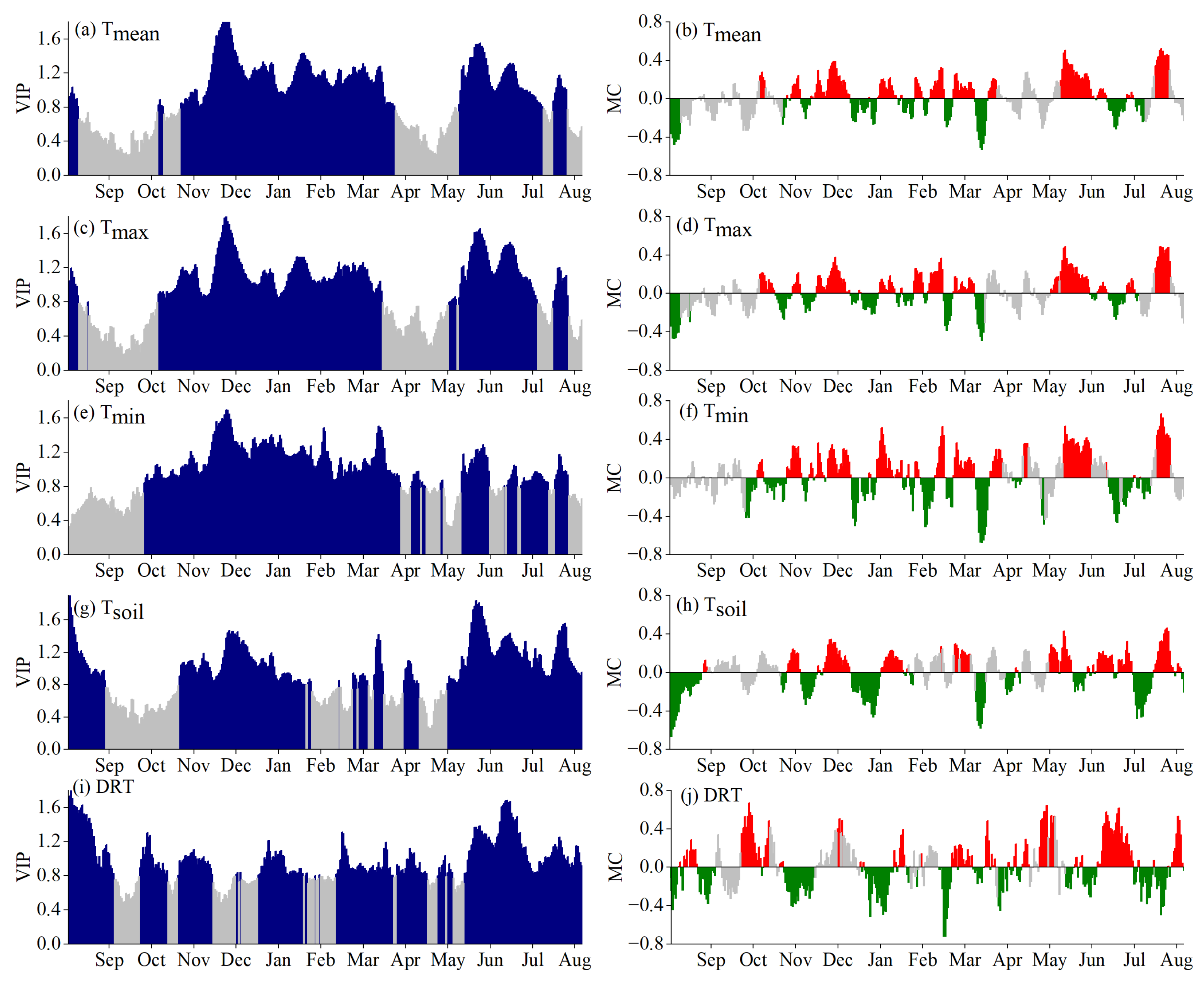
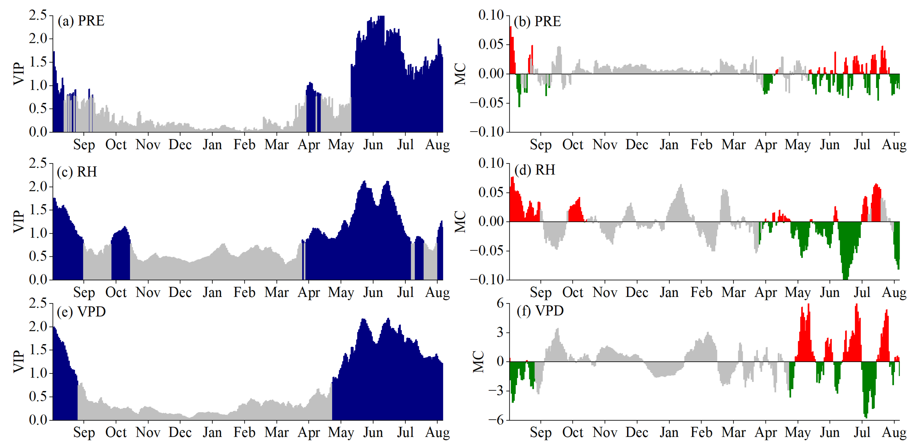
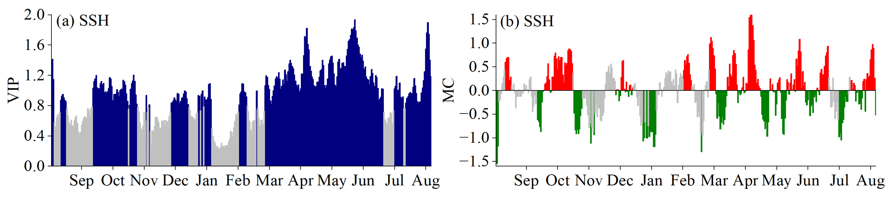
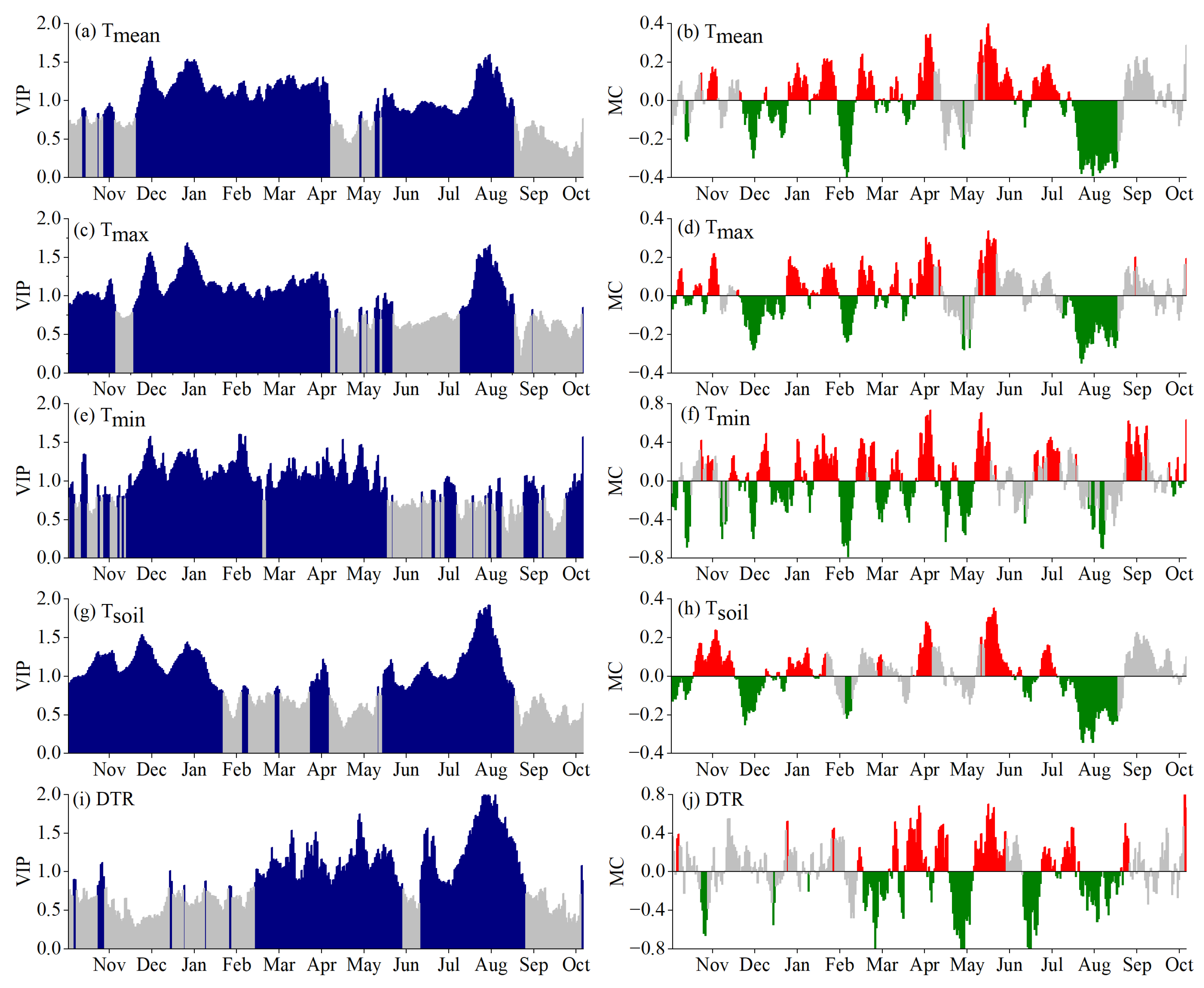
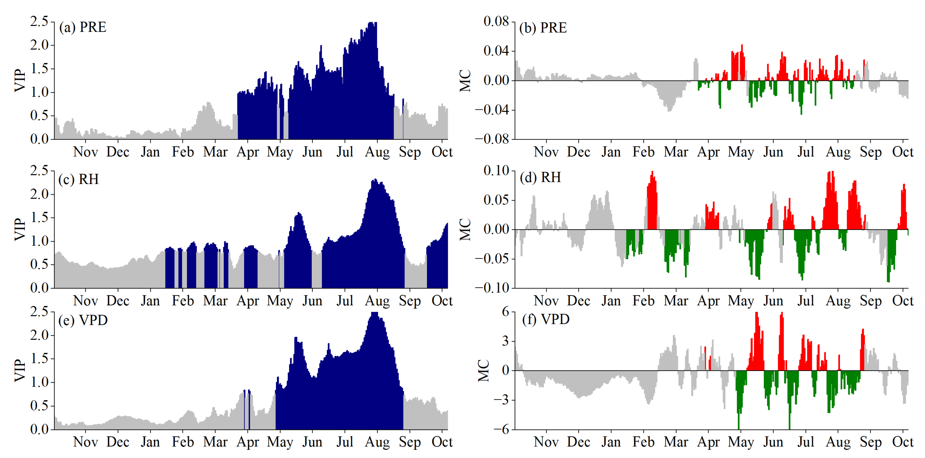
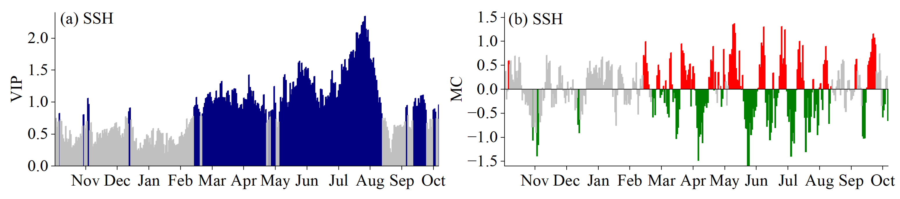
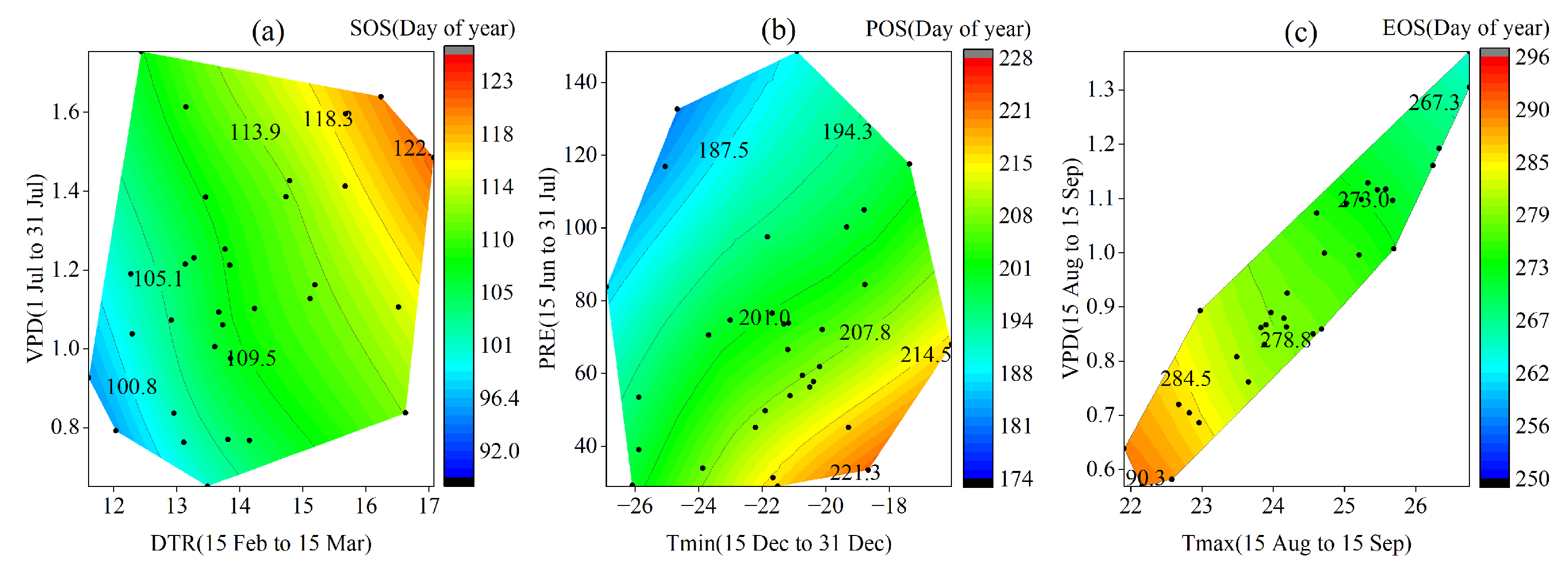
3.2. Critical Periods for SOS Driven by Climatic Factors

According to the VIP and MC values of the PLS, the critical periods, intensities and the directions of the effects of temperature, moisture and light factors between the previous May and April of the year on the SOS were determined (Figure 2, Figure 3 and Figure 4). Temperature was a critical indicator influencing the SOS of S. krylovii. The increase in temperature in cold periods was not conducive to green-up, while it promoted green-up in warm periods.
The PLS regression showed that temperature influenced the SOS throughout winter and spring (Figure 2), with over 78% of VIP values greater than 0.8 between the previous May and April of the year. In addition, the effects of Tmean, Tmax, Tmin, Tsoil and DTR on the SOS were highly consistent. In late January, the effects of Tmean, Tmax, Tmin, Tsoil and DTR on the SOS were mostly positively correlated according to the MC and VIP values (MC > 0, VIP ≥ 0.8). From late March to mid-April, the effects of Tmean, Tmax, Tmin and Tsoil on the SOS were negative (MC < 0, VIP ≥ 0.8), suggesting that the increase in temperature accelerated SOS. Moreover, the DTR from mid-February to mid-March were positive with SOS, indicating that the increase in the DTR induced a delayed SOS. Therefore, late January and late March to mid-April were the two critical periods for the SOS. Mid-February to mid-March was the critical period for the SOS in response to the DTR. Furthermore, the SOS was more closely related to Tmax than to Tmin.
For PRE and VPD, approximately 43% of the VIP values from the previous May to April of the year were greater than 0.8, which was mainly concentrated in the previous June to September. In the previous July, the effects of PRE, RH and VPD on the SOS were consistent (Figure 3). The effects of PRE and RH on SOS were significantly negative (MC < 0, VIP ≥ 0.8) and that of VPD on the SOS was positive (MC > 0, VIP ≥ 0.8). The order of the VIP values was VPD > PRE > RH. Different from PRE and VPD, RH had an influence on the SOS from the previous October to March of the year. The MC values of the SOS affected by RH were mostly positive from the previous November to late January (VIP ≥ 0.8), while the opposite effect occurred between February and March. Therefore, the previous July was a critical period for the SOS response to PRE, RH and VPD. Furthermore, the SOS only responded significantly to RH from the previous November to March of the year.
However, light had different effects on the SOS (Figure 4). From May to April of the year, approximately 61% of the VIP values were greater than 0.8, but the impact periods were more dispersed. The influence of SSH on the SOS was positive between the previous July and mid-August (MC > 0, VIP ≥ 0.8). From mid-March to mid-April, the influence of SSH on the SOS was negative (MC < 0, VIP ≥ 0.8). In general, the influence of SSH on the SOS was the most prominent from March to April.

3.3. Critical Periods of POS Driven by Climatic Factors

Temperature (Tmean, Tmax and Tmin) from the previous September to August of the year affected approximately 64% of the VIP values of the POS, mainly concentrated in the previous December to April and June to July of the year (Figure 5). From mid- to late December, the positive effects of Tmean, Tmax, Tmin and Tsoil on the POS were identified (MC > 0, VIP ≥ 0.8), indicating that the increase in Tmax and Tmin resulted in the delay of the POS. The effects of Tmean, Tmax, Tmin and Tsoil on the POS from mid- to late June were similar to those of the previous mid- to late December. In July, as most of the MC values affected by Tmean, Tmax and Tmin on the POS were negative (MC < 0), the increase in temperature facilitated the advance of the POS. Furthermore, the MC values of Tsoil and the DTR affecting the POS in July were mostly positive, and the VIP values were more than 0.8, indicating that the increase in Tsoil and the DTR induced the delay of the POS. Overall, the previous mid- to late December and mid-June to July were the critical periods affecting the POS. The effect of different temperatures on the POS varied greatly in some critical periods, and the effect of Tmax on the POS was greater than that of Tmin.
Moisture had a greater effect on the POS than temperature, and this pattern was more pronounced. From the previous September to August of the year, moisture (PRE, RH and VPD) affected approximately 32% of the VIP values of the POS, mainly from June to August (Figure 6). From the previous October to April of the year, the effect of moisture on the POS was not significant (VIP < 0.8). From mid-June to late July, most of the MC values affected by PRE and RH on the POS were negative, those affected by VPD were positive, and the VIP values were more than 0.8 or even more than 2 in most periods. The influence of moisture on the POS was relatively clear, and the critical period for moisture to affect the POS was between mid-June and late July.
The VIP values of approximately 65% affected by SSH on the POS from September to August of the year were greater than 0.8, with the period of influence mainly concentrated between April and June (Figure 7). From mid-April to late June, the MC values affected by SSH on the POS were mostly positive, with VIP values exceeding 0.8, indicating that an increase in SSH caused the POS delay during this period. Collectively, SSH had essentially no impact on the POS from the previous December to March of the year, with mid-April to late June being the critical period for affecting the POS.

3.4. Critical Periods of EOS Driven by Climatic Factors

The VIP values of the significant influence of temperature (Tmean, Tmax and Tmin) on EOS from November to October of the year were approximately 68%, mainly from December to April and from August to September (Figure 8). Tmean, Tmax, Tmin, Tsoil and DTR had both consistency and difference in a specific period that affected the EOS. The effects of Tmean, Tmax, Tmin and Tsoil on the EOS were mostly negative from the previous mid-December to late January of the year (MC < 0, VIP > 0.8), indicating that the increase in temperature promoted the advance of the EOS. From mid-August to mid-September, the effects of Tmean, Tmax, Tsoil and DTR on the EOS were highly consistent, while Tmin had no effect on the EOS. In summary, the previous late December to late January and mid-August to mid-September were the critical periods affecting the EOS. The variation in the EOS was better explained by Tmax or DTR.
The precipitation season significantly affected the EOS. The VIP values (VIP ≥ 0.8) of the EOS significantly affected by moisture (PRE, RH and VPD) between the previous November and October of the year were about 38% and were concentrated between May and September (Figure 9). From mid-August to mid-September, most of the MC values affected by PRE and RH were positive, with negative values affected by VPD. The VIP values were more than 0.8 or even more than 2, indicating that the increase in PRE and RH or the decrease in VPD resulted in the delay of EOS. In general, the pattern of moisture impact on the EOS was relatively obvious. Mid-August to mid-September was the critical period affecting the EOS, which indicated that the increase in precipitation in late summer and early autumn was beneficial to the growth of herbaceous plants.
From the previous November to October of the year, 54% of VIP values were greater than 0.8, mainly from mid-March to early September, which indicated the effect of SSH on the EOS throughout the growing season (Figure 10). The influence pattern of SSH effect on the EOS was relatively vague and complex, and the positive and negative ratio of the MC value was similar. From mid-August to late August, the MC values of the influence of SSH on the EOS were mostly negative, which indicated that the increase in SSH resulted in the advance of the EOS. Overall, the influences of SSH on the EOS were the strongest from mid-August to late August, and this period was the critical period affecting the EOS.

3.5. Phenological Responses to Key Climatic Factors

The effects of temperature and moisture on phenology were greater than those of light in a specific period according to Section 3.2, Section 3.3 and Section 3.4. Two critical periods were selected to explore the underlying mechanism of temperature and moisture on the SOS (Figure 11a). The delay in the SOS (red) was not only a response to the DTR from mid-February to mid-March but also a response to moisture in the previous July. A high DTR and low precipitation jointly led to delay of the SOS. Tmin and PRE dominated the variation in the POS (Figure 11b). The EOS responded to temperature and moisture in the two critical periods at some degree (Figure 11c). PRE from mid-August to mid-September has a significantly positive effect on the EOS. The effect of Tmax from mid-August to mid-September on the EOS was regulated by moisture, resulting in no significant advance in the EOS.
Furthermore, stepwise regression analysis was used to identify the ability of climatic factors in critical periods to explain phenological variations (Table 1). The results showed that VPD in the previous July and Tmax in the previous September had significantly positive impacts on the SOS. DTR from mid-February to mid-March in the current year had a significantly positive impact on the SOS, while Tmax from late March to mid-April had the opposite impact. The climatic factors in the four critical periods explained 68.5% of the variation in the SOS. The relative importance order of the four indicators on the SOS was DTR2z–3z > Tmax3x–4z > Tmax9 > VPD7. Tmin from mid-December to late December had a significantly negative impact on the POS. In addition, PRE from mid-June to late July had a significantly negative impact on the POS. The effect of PRE on POS was greater than Tmin, together explaining 52.1% of the variation in the POS. Tmax from mid-August to mid-September had a significantly negative impact on the EOS, which could explain 49.3% of the variations in the EOS.
Tmax9 represents maximum air temperature in September of the previous year; Tmax3x–4z indicates maximum air temperature from late March to mid-April; DTR2z–3z denotes diurnal temperature range from mid-February to mid-March; VPD7 is saturated water vapor pressure difference in July of the previous year. Tmin12z–12d represents minimum air temperature from the previous mid-December to late December; PRE6z–7 is the precipitation from mid-June to mid-July of the current year. Tmax8z–9z is the maximum temperature from mid-August to mid-September of the current year.

4. Discussion

4.1. Critical Periods of Climatic Factors Driving Phenology

The influence of climatic factors on grassland phenology had a time-lag effect [10]. For instance, in Northeast China, the precipitation from September to December of the previous year advanced the SOS of the next year, and increases in precipitation advanced the SOS [52]. Therefore, for the analyses of phenology and climatic factors, climate factors, i.e., Tmean, Tmax, Tmin, Tsoil, DTR, PRE, VPD, RH and SSH, were selected for the 12 months prior to the grassland SOS, POS and EOS. In most temperate and northern regions, late winter and spring temperatures play the most important roles in driving the SOS [45]. Tao et al. [11] showed that the SOS was mainly triggered by preseason temperature and increased temperature leading to an earlier SOS. The most notable difference from previous studies is that the present study identified critical periods for the SOS, POS and EOS responses to potential climatic factors. The impacts of climate variability on grassland phenology varied with growth stages. We identified that July in the previous year, September in the previous year, mid-February to mid-March in the current year and late March to mid-April in the previous year were the four critical periods affecting the SOS, which means that the phenological variations in S. krylovii were the result of the combined effects of climatic conditions from the previous year and the current year. Different from previous studies, this study found that the increase in DTR from mid-February to mid-March was the dominant factor and period for a delayed SOS. In addition, the increase in DTR was mainly caused by the greater increase in Tmax than Tmin, which also suggested that DTR may reflect asymmetric effects of daytime and night-time warming. Huang et al. [45] also emphasized the importance of a preseason DTR in regulating the SOS, which was essential for understanding temperature indicators contributing to the changes in the SOS. However, the effects of Tmax and Tmin on the SOS were not uniform. Previous studies showed that interannual anomalies of the SOS in woody plants were mainly caused by Tmax rather than by Tmin in Europe and the United States [53], which were consistent with our findings. In contrast, Tmin played a major role in controlling the SOS of Kobresia humilis in the Tibetan Plateau [40]. In addition, a better presentation of phenological characteristics could be achieved by including variations in Tmax and Tmin in the model than by only using Tmean [1]. Meanwhile, Piao et al. [53] suggested to use Tmax to improve the performance of phenology modules in current Earth system models.
Previous studies often ignored the effect of moisture on the phenology of grassland plants, which caused great uncertainty to the accurate assessment of grassland phenology [26]. This study found that the influence of RH in winter and spring on the SOS was significant, implying that the description of the SOS by RH in this period was stronger than that of precipitation, providing a theoretical basis for the development of SOS models. The critical period affecting the POS was mid-June to late July, during which the increase in precipitation promoted the advance of the POS. The increase in Tmin in the cold period (December) induced the POS delay. Compared with temperature and light, moisture had a greater impact on the POS of S. krylovii plants. Mid-August to mid-September was the critical period affecting the EOS (Figure 11). During this period, Tmax was negatively correlated with precipitation, which further indicated that the increase in temperature led to a water deficit and eventually induced the early appearance of the EOS. SSH in August had a negative impact on the EOS, possibly due to increased solar radiation and evapotranspiration in late summer and early autumn, limiting the use ability of vegetation for water resources [54]. Therefore, the effects of moisture and light should also be considered in the EOS models [55].

4.2. Response Mechanism of Phenology to Climatic Factors

In recent decades, some studies have shown that warming in the middle and high latitudes of the Northern Hemisphere causes an early SOS and a late EOS [11], ultimately leading to a longer growth cycle. However, climatic controls on the SOS of grassland plants are location specific [31]. In addition, the effect of climate warming on the advanced SOS was not as obvious as in previous decades [17]. Ren et al. [56] highlighted the important role of thermal-moisture background in controlling the spatial pattern of the SOS in response to climate change. In semi-arid regions, both preseason temperature and precipitation affected the SOS, leading to a complex response of the SOS to climate change [57]. Adequate water supply usually promoted early plant growth in arid and semi-arid regions under suitable high-temperature conditions [32]. In water-deficient regions, climate warming exacerbated drought stress and delayed plant growth [17,58]. Therefore, precipitation pattern appears to be a dominant climatic driver of interannual variation of plant phenology in arid and semi-arid regions [20,24], with temperature triggering the SOS only when the water supply is adequate [56]. In other words, precipitation had both direct and indirect effects on the SOS [57]. The SOS showed a delayed trend in the last 34 years, while the POS and EOS did not show an obvious early trend in semi-arid region (Figure 1). This result was consistent with the research results from [15], Yu et al. [29] showed a similar trend of the SOS in the Qinghai-Tibet Plateau. The changing character of the delayed SOS may be the result of plants responding to a warm and dry climatic context.
Furthermore, the antagonistic effects of cold accumulation and thermal forcing on the SOS have been widely used to explain the impact of climate variation on plant phenology. It is generally believed that increasing winter temperature delays the SOS by reducing cold temperature demand [29], while increasing spring temperature promotes the SOS. Therefore, to some extent, the delay or advance of the SOS depends on the trade-off between the two mechanisms [35,40,59]. However, Wang et al. [42] showed that the effect of preseason cold accumulation in Inner Mongolia on the SOS of individual grass species was quite limited. Specifically, the trade-off mechanism between cold accumulation and thermal forcing may be more appropriate to explain the response of the SOS to climate warming in humid climate regions.
Kang et al. [15] believed that the decrease in spring precipitation delayed the SOS of grassland plants, while the decrease in autumn precipitation advanced the EOS [25]. Liu et al. [55] showed that the effect of preseason precipitation on the EOS of grassland plants was positive, which may be related to the effect of water stress on plant growth in autumn. Our measured meteorological data showed that VPD exhibited a significant increasing trend in July over the past 34 years, and DTR showed an increasing trend from mid-February to mid-March. In addition, the DTR was significantly negatively correlated with RH in March during that period, and the interannual variation in climate showed a significant warming-drying trend in semi-arid regions [60], which was not conducive to plant growth and eventually induced the delay in the SOS. It was also found that warming delayed plant growth in warm and dry years and accelerated plant growth in cold and wet years [17]. Therefore, moisture in arid and semi-arid regions may be a precondition rather than a supplementary condition for driving temperature in triggering the SOS [31]. Our results provide an important basis for the construction of plant phenology models. DTR can be used as a supplementary ecological index for heat requirement-based phenology models to simulate and predict the SOS [45]. Summer precipitation dominated the change in the POS in semi-arid region. Therefore, it is necessary to consider precipitation in models for predicting the POS of grassland plants [27,61].

5. Conclusions

The critical periods of climatic factors driving the phenology of S. krylovii were identified, and their underling mechanisms were explored in semi-arid regions in Inner Mongolia. There was a significant delayed trend in SOS, while POS and EOS did not show a clear advanced trend. It was found that the influence direction and intensity of climatic variables in different periods on different phenology were heterogeneous. Moisture conditions in the previous year and thermal conditions in the current year together affected the SOS. In addition, the preseason DTR (mid-February to March) played a leading role in delaying SOS. The preseason PRE (mid-June to late July) and Tmax (mid-August to mid-September) dominated the POS and EOS, respectively. In summary, adding meteorological constraints identified by PLS regression to existing grassland phenological models is expected to improve the accuracy of the phenology models.

Author Contributions

Conceptualization, E.L., G.Z. and Q.H.; methodology, E.L., G.Z. and B.W.; validation: E.L., G.Z., Q.H. and W.G.; formal analysis, E.L.; investigation, E.L. and W.G.; writing—original draft preparation, E.L. and G.Z.; writing—review and editing, E.L., G.Z. and H.Z.; funding acquisition, G.Z. All authors have read and agreed to the published version of the manuscript.

Funding

This research was funded by the National Key Research and Development Program of China (2018YFD0606103) and by the National Natural Science Foundation of China (42130514).

Institutional Review Board Statement

Not applicable.

Informed Consent Statement

Not applicable.

Data Availability Statement

Data available on request.

Acknowledgments

We sincere thanks go to the editor and anonymous reviewers for their thoughtful comments that improved this manuscript.

Conflicts of Interest

The authors declare no conflict of interest.

References

  1. Li, Q.Y.; Xu, L.; Pan, X.B.; Zhang, L.Z.; Li, C.; Yang, N.; Qi, J.G. Modeling phenological responses of Inner Mongolia grassland species to regional climate change. Environ. Res. Lett. 2016, 11, 015002. [Google Scholar] [CrossRef]
  2. Ren, S.L.; Yi, S.H.; Peichl, M.; Wang, X.Y. Diverse responses of vegetation phenology to climate change in different grasslands in Inner Mongolia during 2000. Remote Sens. 2017, 10, 17. [Google Scholar] [CrossRef]
  3. Cao, R.Y.; Chen, J.; Shen, M.G.; Tang, T.H. An improved logistic method for detecting spring vegetation phenology in grasslands from MODIS EVI time-series data. Agric. For. Meteorol. 2015, 200, 9–20. [Google Scholar] [CrossRef]
  4. Wang, G.C.; Huang, Y.; Wei, Y.R.; Zhang, W.; Li, T.T.; Zhang, Q. Inner Mongolian grassland plant phenological changes and their climatic drivers. Sci. Total Environ. 2019, 683, 1–8. [Google Scholar] [CrossRef]
  5. Ibañez, M.; Altimir, N.; Ribas, A.; Eugster, W.; Sebastià, M.T. Phenology and plant functional type dominance drive CO2 exchange in seminatural grasslands in the Pyrenees. J. Agric. Sci. 2020, 158, 3–14. [Google Scholar] [CrossRef]
  6. Xu, L.L.; Niu, B.; Zhang, X.Z.; He, Y.T. Dynamic threshold of carbon phenology in two cold temperate grasslands in China. Remote Sens. 2021, 13, 574. [Google Scholar] [CrossRef]
  7. Du, Q.; Liu, H.Z.; Li, Y.H.; Xu, L.J.; Diloksumpun, S. The effect of phenology on the carbon exchange process in grassland and maize cropland ecosystems across a semiarid area of China. Sci. Total Environ. 2019, 695, 133868. [Google Scholar] [CrossRef] [PubMed]
  8. Ren, S.L.; Chen, X.Q.; Lang, W.G.; Schwartz, M.D. Climatic controls of the spatial patterns of vegetation phenology in midlatitude grasslands of the Northern Hemisphere. J. Geophys. Res. Biogeosciences 2018, 123, 2323–2336. [Google Scholar] [CrossRef]
  9. Shen, X.J.; Liu, B.H.; Henderson, M.; Wang, L.; Wu, Z.F.; Wu, H.T.; Jiang, M.; Lu, X.G. Asymmetric effects of daytime and nighttime warming on spring phenology in the temperate grasslands of China. Agric. For. Meteorol. 2018, 259, 240–249. [Google Scholar] [CrossRef]
  10. Zhang, R.P.; Guo, J.; Liang, T.G.; Feng, Q.S. Grassland vegetation phenological variations and responses to climate change in the Xinjiang region, China. Quatern. Int. 2019, 513, 56–65. [Google Scholar] [CrossRef]
  11. Tao, Z.X.; Wang, H.J.; Liu, Y.C.; Xu, Y.J.; Dai, J.H. Phenological response of different vegetation types to temperature and precipitation variations in northern China during 1982. Int. J. Remote Sens. 2017, 38, 3236–3252. [Google Scholar] [CrossRef]
  12. Wang, S.Y.; Yang, B.Y.; Yang, Q.C.; Lu, L.L.; Wang, X.Y.; Peng, Y.Y. Temporal trends and spatial variability of vegetation phenology over the Northern Hemisphere during 1982. PLoS ONE 2016, 11, e0157134. [Google Scholar]
  13. Wang, Y.Q.; Luo, Y.; Shafeeque, M. Interpretation of vegetation phenology changes using daytime and night-time temperatures across the Yellow River Basin, China. Sci. Total Environ. 2019, 693, 133553. [Google Scholar] [CrossRef] [PubMed]
  14. Yang, J.L.; Dong, J.W.; Xiao, X.M.; Dai, J.H.; Wu, C.Y.; Xia, J.Y.; Zhao, G.S.; Zhao, M.M.; Li, Z.L.; Zhang, Y.; et al. Divergent shifts in peak photosynthesis timing of temperate and alpine grasslands in China. Remote Sens. Environ. 2019, 233, 111395. [Google Scholar] [CrossRef]
  15. Kang, W.P.; Wang, T.; Liu, S.L. The response of vegetation phenology and productivity to drought in semi-arid regions of Northern China. Remote Sens. 2018, 10, 727. [Google Scholar] [CrossRef]
  16. Wang, G.C.; Huang, Y.; Wei, Y.R.; Zhang, W.; Li, T.T.; Zhang, Q. Climate warming does not always extend the plant growing season in Inner Mongolian grasslands: Evidence from a 30-year in situ observations at eight experimental sites. J. Geophys. Res. Biogeosciences 2019, 124, 2364–2378. [Google Scholar] [CrossRef]
  17. Ganjurjav, H.; Gornish, E.S.; Hu, G.Z.; Schwartz, M.W.; Wan, Y.F.; Li, Y.; Gao, Q.Z. Warming and precipitation addition interact to affect plant spring phenology in alpine meadows on the central Qinghai-Tibetan Plateau. Agric. For. Meteorol. 2020, 287, 107943. [Google Scholar] [CrossRef]
  18. Whittington, H.R.; Tilman, D.; Wragg, P.D.; Powers, J.S. Phenological responses of prairie plants vary among species and year in a three-year experimental warming study. Ecosphere 2015, 6, 1–15. [Google Scholar] [CrossRef]
  19. Fu, Y.H.; Zhou, X.C.; Li, X.X.; Zhang, Y.R.; Geng, X.J.; Hao, F.H.; Zhang, X.; Hanninen, H.; Guo, Y.H.; De Boeck, H.J. Decreasing control of precipitation on grassland spring phenology in temperate China. Glob. Ecol. Biogeogr. 2021, 30, 490–499. [Google Scholar] [CrossRef]
  20. Ren, S.L.; Chen, X.; An, S. Assessing plant senescence reflectance index-retrieved vegetation phenology and its spatiotemporal response to climate change in the Inner Mongolian Grassland. Int. J. Biometeorol. 2017, 61, 601–612. [Google Scholar] [CrossRef]
  21. Zhou, T.; Cao, R.Y.; Wang, S.P.; Chen, J.; Tang, Y.H. Responses of green-up dates of grasslands in China and woody plants in Europe to air temperature and precipitation: Empirical evidences based on survival analysis. Chin. J. Plant Ecol. 2018, 42, 526–538. (In Chinese) [Google Scholar]
  22. Guo, J.; Yang, X.C.; Niu, J.M.; Jin, Y.X.; Xu, B.; Shen, G.; Zhang, W.B.; Zhao, F.; Zhang, Y.J. Remote sensing monitoring of green-up dates in the Xilingol grasslands of northern China and their correlations with meteorological factors. Int. J. Remote Sens. 2018, 40, 2190–2211. [Google Scholar] [CrossRef]
  23. Lesica, P.; Kittelson, P.M. Precipitation and temperature are associated with advanced flowering phenology in a semi-arid grassland. J. Arid Environ. 2010, 74, 1013–1017. [Google Scholar] [CrossRef]
  24. Shen, M.G.; Tang, Y.H.; Chen, J.; Zhu, X.L.; Zheng, Y.H. Influences of temperature and precipitation before the growing season on spring phenology in grasslands of the central and eastern Qinghai-Tibetan Plateau. Agric. For. Meteorol. 2011, 151, 1711–1722. [Google Scholar] [CrossRef]
  25. An, S.; Chen, X.Q.; Zhang, X.Y.; Lang, W.G.; Ren, S.L.; Xu, L. Precipitation and minimum temperature are primary climatic controls of alpine grassland autumn phenology on the Qinghai-Tibet Plateau. Remote Sens. 2020, 12, 431. [Google Scholar] [CrossRef]
  26. Liu, Q.; Fu, Y.H.; Liu, Y.; Janssens, I.A.; Piao, S. Simulating the onset of spring vegetation growth across the Northern Hemisphere. Glob. Chang. Biol. 2018, 24, 1342–1356. [Google Scholar] [CrossRef]
  27. Wang, G.C.; Luo, Z.K.; Huang, Y.; Xia, X.G.; Wei, Y.R.; Lin, X.H.; Sun, W.J. Preseason heat requirement and days of precipitation jointly regulate plant phenological variations in Inner Mongolian grassland. Agric. For. Meteorol. 2022, 314, 108783. [Google Scholar] [CrossRef]
  28. Fu, Y.H.; Piao, S.L.; Vitasse, Y.; Zhao, H.; De Boeck, H.J.; Liu, Q.; Yang, H.; Weber, U.; Hanninen, H.; Janssens, I.A. Increased heat requirement for leaf flushing in temperate woody species over 1980–2012: Effects of chilling, precipitation and insolation. Glob. Chang. Biol. 2015, 21, 2687–2697. [Google Scholar] [CrossRef]
  29. Yu, H.Y.; Luedeling, E.; Xu, J.C. Winter and spring warming result in delayed spring phenology on the Tibetan Plateau. Proc. Natl. Acad. Sci. USA 2010, 107, 22151–22156. [Google Scholar] [CrossRef] [PubMed]
  30. Yu, H.Y.; Xu, J.C.; Okuto, E.; Luedeling, E. Seasonal response of grasslands to climate change on the Tibetan Plateau. PLoS ONE 2012, 7, e49230. [Google Scholar] [CrossRef] [PubMed]
  31. Chen, X.Q.; Li, J.; Xu, L.; Liu, L.; Ding, D. Modeling greenup date of dominant grass species in the Inner Mongolian grassland using air temperature and precipitation data. Int. J. Biometeorol. 2014, 58, 463–471. [Google Scholar] [CrossRef] [PubMed]
  32. Ren, S.L.; Li, Y.T.; Peichl, M. Diverse effects of climate at different times on grassland phenology in mid-latitude of the Northern Hemisphere. Ecol. Indic. 2020, 113, 106260. [Google Scholar] [CrossRef]
  33. Porker, K.; Coventry, S.; Fettell, N.A.; Cozzolino, D.; Eglinton, J. Using a novel PLS approach for envirotyping of barley phenology and adaptation. Field Crops Res. 2020, 246, 107697. [Google Scholar] [CrossRef]
  34. Wang, X.; Du, P.J.; Chen, D.M.; Lin, C.; Zheng, H.R.; Guo, S.C. Characterizing urbanization-induced land surface phenology change from time-series remotely sensed images at fine spatio-temporal scale: A case study in Nanjing, China (2001–2018). J. Clean. Prod. 2020, 274, 122487. [Google Scholar] [CrossRef]
  35. Guo, L.; Cheng, J.M.; Luedeling, E.; Koerner, S.E.; He, J.S.; Xu, J.C.; Gang, C.C.; Li, W.; Luo, R.M.; Peng, C.H. Critical climate periods for grassland productivity on China’s Loess Plateau. Agric. For. Meteorol. 2017, 233, 101–109. [Google Scholar] [CrossRef]
  36. Guo, L.; Dai, J.H.; Ranjitkar, S.; Xu, J.C.; Luedeling, E. Response of chestnut phenology in China to climate variation and change. Agric. For. Meteorol. 2013, 180, 164–172. [Google Scholar] [CrossRef]
  37. Luedeling, E.; Guo, L.; Dai, J.H.; Leslie, C.; Blanke, M.M. Differential responses of trees to temperature variation during the chilling and forcing phases. Agric. For. Meteorol. 2013, 181, 33–42. [Google Scholar] [CrossRef]
  38. Luedeling, E.; Kunz, A.; Blanke, M.M. Identification of chilling and heat requirements of cherry trees-a statistical approach. Int. J. Biometeorol. 2013, 57, 679–689. [Google Scholar] [CrossRef] [PubMed]
  39. Guo, L.; Dai, J.H.; Wang, M.C.; Xu, J.C.; Luedeling, E. Responses of spring phenology in temperate zone trees to climate warming: A case study of apricot flowering in China. Agric. For. Meteorol. 2015, 201, 1–7. [Google Scholar] [CrossRef]
  40. Li, X.T.; Guo, W.; Chen, J.; Ni, X.N.; Wei, X.Y. Responses of vegetation green-up date to temperature variation in alpine grassland on the Tibetan Plateau. Ecol. Indic. 2019, 104, 390–397. [Google Scholar] [CrossRef]
  41. Rosenzweig, C.; Karoly, D.; Vicarelli, M.; Neofotis, P.; Wu, Q.G.; Casassa, G.; Menzel, A.; Root, T.L.; Estrella, N.; Seguin, B.; et al. Attributing physical and biological impacts to anthropogenic climate change. Nature 2008, 453, 353–357. [Google Scholar] [CrossRef] [PubMed]
  42. Wang, G.C.; Xiao, M.J.; Xia, X.G.; Huang, Y.; Luo, Z.K.; Wei, Y.R.; Zhang, W. Chilling accumulation is not an effective predictor of vegetation green-up date in Inner Mongolian grasslands. Geophys. Res. Lett. 2021, 49, e2021GL096558. [Google Scholar] [CrossRef]
  43. China Meteorological Administration. Observation Criterion of Agricultural Meteorology; China Meteorological Press: Beijing, China, 1993. (In Chinese) [Google Scholar]
  44. Chen, X.Q.; An, S.; Inouye, D.W.; Schwartz, M.D. Temperature and snowfall trigger alpine vegetation green-up on the world’s roof. Glob. Chang. Biol. 2015, 21, 3635–3646. [Google Scholar] [CrossRef]
  45. Huang, Y.; Jiang, N.; Shen, M.G.; Guo, L. Effect of preseason diurnal temperature range on the start of vegetation growing season in the Northern Hemisphere. Ecol. Indic. 2020, 112, 106161. [Google Scholar] [CrossRef]
  46. Jolly, W.M.; Nemani, R.; Running, S.W. A generalized, bioclimatic index to predict foliar phenology in response to climate. Glob. Chang. Biol. 2005, 11, 619–632. [Google Scholar] [CrossRef]
  47. Allen, R.G.; Pereira, L.S.; Raes, D.; Smith, M. Crop evapotranspiration-guidelines for computing crop water requirements-FAO irrigation and drainage paper. FAO Rome 1998, 300, D05109. [Google Scholar]
  48. Yuan, W.P.; Zheng, Y.; Piao, S.L.; Ciais, P.; Lombardozzi, D.; Wang, Y.P.; Ryu, Y.; Chen, G.X.; Dong, W.J.; Hu, Z.M.; et al. Increased atmospheric vapor pressure deficit reduces global vegetation growth. Sci. Adv. 2019, 5, eaax1396. [Google Scholar] [CrossRef]
  49. Luedeling, E.; Gassner, A. Partial Least Squares Regression for analyzing walnut phenology in California. Agric. For. Meteorol. 2012, 158–159, 43–52. [Google Scholar] [CrossRef]
  50. Pak, D.; Biddinger, D.; Bjørnstad, O.N. Local and regional climate variables driving spring phenology of tortricid pests: A 36year study. Ecol. Entomol. 2018, 44, 367–379. [Google Scholar] [CrossRef]
  51. Yin, C.; Yang, Y.P.; Yang, F.; Chen, X.N.; Xin, Y.; Luo, P.X. Diagnose the dominant climate factors and periods of spring phenology in Qinling Mountains, China. Ecol. Indic. 2021, 131, 108211. [Google Scholar] [CrossRef]
  52. Zhao, J.J.; Wang, Y.Y.; Zhang, Z.X.; Zhang, H.Y.; Guo, X.Y.; Yu, S.; Du, W.L.; Huang, F. The variations of land surface phenology in Northeast China and its responses to climate change from 1982 to 2013. Remote Sens. 2016, 8, 400. [Google Scholar] [CrossRef]
  53. Piao, S.; Tan, J.; Chen, A.; Fu, Y.H.; Ciais, P.; Liu, Q.; Janssens, I.A.; Vicca, S.; Zeng, Z.; Jeong, S.J.; et al. Leaf onset in the northern hemisphere triggered by daytime temperature. Nat. Commun. 2015, 6, 6911. [Google Scholar] [CrossRef] [PubMed]
  54. Zhang, Q.; Kong, D.D.; Shi, P.J.; Singh, V.P.; Sun, P. Vegetation phenology on the Qinghai-Tibetan Plateau and its response to climate change (1982–2013). Agric. For. Meteorol. 2018, 248, 408–417. [Google Scholar] [CrossRef]
  55. Liu, Q.; Fu, Y.H.; Zeng, Z.; Huang, M.; Li, X.; Piao, S.L. Temperature, precipitation, and insolation effects on autumn vegetation phenology in temperate China. Glob. Chang. Biol. 2016, 22, 644–655. [Google Scholar] [CrossRef]
  56. Ren, S.L.; Chen, X.Q.; Pan, C.C. Temperature-precipitation background affects spatial heterogeneity of spring phenology responses to climate change in northern grasslands (30° N–55° N). Agric. For. Meteorol. 2022, 315, 108816. [Google Scholar] [CrossRef]
  57. Shen, M.G.; Piao, S.L.; Cong, N.; Zhang, G.X.; Jassens, I.A. Precipitation impacts on vegetation spring phenology on the Tibetan P lateau. Glob. Chang. Biol. 2015, 21, 3647–3656. [Google Scholar] [CrossRef]
  58. Xin, Q.C.; Broich, M.; Zhu, P.; Gong, P. Modeling grassland spring onset across the Western United States using climate variables and MODIS-derived phenology metrics. Remote Sens. Environ. 2015, 161, 63–77. [Google Scholar] [CrossRef]
  59. Fu, Y.H.; Campioli, M.; Deckmyn, G.; Janssens, I.A. Sensitivity of leaf unfolding to experimental warming in three temperate tree species. Agric. For. Meteorol. 2013, 181, 125–132. [Google Scholar] [CrossRef]
  60. Xiao, F.; Sang, J.; Wang, H.M. Effects of climate change on typical grassland plant phenology in Ewenli, Inner Mongolia. Acta Ecol. Sin. 2020, 40, 2784–2792. (In Chinese) [Google Scholar]
  61. Tao, Z.X.; Dai, J.H.; Wang, H.J.; Huang, W.J.; Ge, Q.S. Spatiotemporal changes in the bud-burst date of herbaceous plants in Inner Mongolia grassland. J. Geogr. Sci. 2020, 29, 2122–2138. [Google Scholar] [CrossRef]
Figure 1. The dynamic trends of the phenology for S. krylovii from 1985–2018. (a,b) represent the distribution frequency and changing trend for the start of the growing season (SOS). (c,d) represent the distribution frequency and changing trend for the peak of the growing season (POS). (e,f) represent the distribution frequency and changing trend for the end of the growing season (EOS).
Agronomy 12 01906 g001
Figure 2. Results of partial least squares (PLS) regression correlating the start of the growing season (SOS) from 1985–2018 with 31-day running means of climatic factors. (a,b) Daily mean air temperature (Tmean), (c,d) daily maximum air temperature (Tmax), (e,f) daily minimum air temperature (Tmin), (g,h) daily soil surface temperature (Tsoil) and (i,j) diurnal temperature range (DTR) from the previous May to April of the year. (a,c,e,g,i) indicate the variable importance in projection (VIP): blue indicates VIP ≥ 0.8, grey indicates VIP < 0.8; (b,d,f,h,j) indicate the standardized model coefficients (MC): red indicates a positive model coefficient, green indicates a negative model coefficient, and grey indicates an insignificant model coefficient. Same as below.
Agronomy 12 01906 g002
Figure 3. Results of partial least squares (PLS) regression correlating the start of the growing season (SOS) from 1985–2018 with 31-day running means of climatic factors. (a,b) Daily precipitation (PRE), (c,d) relative humidity (RH) and (e,f) vapor pressure deficit (VPD) from the previous May to April of the year.
Agronomy 12 01906 g003
Figure 4. Results of partial least squares (PLS) regression correlating the start of the growing season (SOS) from 1985–2018 with 31-day running means of climatic factors. (a,b) Sunshine hours (SSH) from the previous May to April of the year.
Agronomy 12 01906 g004
Figure 5. Results of partial least squares (PLS) regression correlating the peak of the growing season (POS) from 1985–2018 with 31-day running means of climatic factors. (a,b) Daily mean air temperature (Tmean), (c,d) daily maximum air temperature (Tmax), (e,f) daily minimum air temperature (Tmin), (g,h) daily surface temperature (Tsoil) and (i,j) diurnal temperature range (DTR) from the previous September to August of the year.
Agronomy 12 01906 g005
Figure 6. Results of partial least squares (PLS) regression correlating the peak of the growing season (POS) from 1985–2018 with 31-day running means of climatic factors. (a,b) Daily precipitation (PRE), (c,d) relative humidity (RH) and (e,f) vapor pressure deficit (VPD) from the previous September to August of the year.
Agronomy 12 01906 g006
Figure 7. Results of partial least squares (PLS) regression correlating the peak of the growing season (POS) from 1985–2018 with 31-day running means of climatic factors. (a,b) Sunshine hours (SSH) from the previous September to August of the year.
Agronomy 12 01906 g007
Figure 8. Results of partial least squares (PLS) regression correlating the end of the growing season (EOS) from 1985–2018 with 31-day running means of climatic factors. (a,b) Daily mean air temperature (Tmean), (c,d) daily maximum air temperature (Tmax), (e,f) daily minimum air temperature (Tmin), (g,h) daily soil surface temperature (Tsoil) and (i,j) diurnal temperature range (DTR) from the previous November to October of the year.
Agronomy 12 01906 g008
Figure 9. Results of partial least squares (PLS) regression correlating the end of the growing season (EOS) from 1985–2018 with 31-day running means of climatic factors. (a,b) Daily precipitation (PRE), (c,d) daily relative humidity (RH) and (e,f) vapor pressure deficit (VPD) from the previous November to October of the year.
Agronomy 12 01906 g009
Figure 10. Results of partial least squares (PLS) regression correlating the end of the growing season (EOS) from 1985–2018 with 31-day running means of climatic factors. (a,b) Sunshine hours (SSH) from the previous November to October of the year.
Agronomy 12 01906 g010
Figure 11. The combined response of the start, peak and end of the growing season (SOS, POS and EOS) to temperature and moisture during the critical periods. (a) The start of the growing season (SOS), (b) the peak of the growing season (POS) and (c) the end of the growing season (EOS). Variation in colour reflects changes in the phenology, and the black dots represent the phenology records from 1985–2018.
Agronomy 12 01906 g011
Table 1. Parameters of stepwise regression for phenology and climatic factors in critical periods.
PhenologyRegression Model (Standard Coefficients)FpR2
SOSSOS = 0.292 × Tmax9−0.422 × Tmax3x–4z +0.672 × DTR2z–3z + 0.276 × VPD714.6660.0000.685
POSPOS = 0.475 × Tmin12z–12d −0.600 × PRE6z-715.8000.0000.521
EOSEOS = −0.702 × Tmax8z–9z13.6020.0020.493
Publisher’s Note: MDPI stays neutral with regard to jurisdictional claims in published maps and institutional affiliations.

