1. Introduction
Phenology is the study of the timing of recurring biological events in the animal and plant world, the causes of their timing with regard to biotic and abiotic forces, and the interrelation among phases of the same or different species [
1,
2].
If the sequence of phenological stages is pre-ordered by plant genetics, the rate of development is strongly affected by the evolution of environmental conditions such as atmospheric variables (solar radiation, temperature, air humidity, etc.), soil water availability, nutrients availability and interactions with other living beings [
3,
4]. As stated by Menzel et al. [
5], in most of the cases, phenology is mainly driven by temperature and/or day length, both varying across latitudes and altitudes. Temperature is the strongest determinant of plant phenology, regardless of species [
6]. Each species is characterized by cardinal and optimal ranges of temperature, affecting the rate of development [
7,
8,
9]. Photoperiod plays a less universal role. It does not affect all developmental transitions, and species differ in their sensitivity to this cue. It could play a role in growth cessation, budset, dormancy induction and leaf senescence. Furthermore, photoperiod can also interact with temperature and alter the development rate [
6].
Finally, as stated in the work of Chuine and Régnière [
6], nutrients and water availability marginally affect phenology timing, except under extreme conditions.
Due to this close relationship between phenological timing variations and meteorological conditions, phenology is also of great interest to climate change studies [
5,
6,
10,
11,
12,
13,
14,
15,
16]. In this sense, an increase in the understanding of relationships between phenology and the structure and function of ecosystems can help inform adaptive management of natural resources [
17]. In the specific case of agriculture, phenological monitoring is largely adopted, mainly for advisory services as decision support information. Traditional phenology is based on regular observations of commonly defined phenological stages, which are recorded in rather long time series, allowing for spatio-temporal analyses of their patterns. Although more advanced earth observation techniques are increasingly applied to monitor vegetation development [
18,
19], phenological time series are fundamental for the development of models able to produce information layers, describing the evolution of plants during the season and predicting the date of occurrence of relevant phenological stages.
In terms of research, most studies focus on major high-income crops, such as vineyards [
20,
21,
22,
23], cereals [
24,
25,
26] and orchards [
27,
28,
29,
30,
31], but also forests are investigated [
32,
33,
34]. Among these, black locust (
Robinia pseudoacacia L.) trees are noticeable for their economic and scientific interest.
Robinia pseudoacacia L. belongs to the Fabaceae family; it is known as “false acacia” in Europe and as “black locust” in the USA. It originated in North America and was imported all over Europe in the early 17th century. In many European countries, it is naturalized and widespread thanks to its ability to adapt to different environmental and soil conditions [
35]. In Italy,
R. pseudocacia was introduced in 1662 in the botanical garden of Padua and it is currently naturalized throughout the whole territory [
36].
R. pseudoacacia is a light-demanding pioneer species, which requires well-drained sites and is drought resistant. Its distribution in Central Europe is constrained by frost, mainly in late spring [
37]. It is widely used for its wood and for its capacity to colonize degraded areas [
38] as a nitrogen-fixing species for waste land, for erosion prevention and control and for carbon sequestration; moreover, it is used as an ornamental tree in parks and gardens, also as a street tree because it can withstand air pollution and salinity, therefore it thrives in the urban environment [
39]. Furthermore, it can provide information about climate change impacts due to its large distribution throughout the world as planted and naturalized trees [
40]. Finally,
R. pseudoacacia is widely exploited in Italy (mainly in the Northern areas) as an excellent melliferous plant: the average Italian production of black locust honey is 11,590 t/year, estimated from the number of hives in the main productive regions and the average yield of 25 kg/hive [
41], which is approximately one half of the Hungarian production of 25,000 t/year [
42]; in fact, Hungary produces about 40–50% of European black locust honey [
37].
Relatively few studies have investigated the phenology of black locust [
40,
43,
44]. It is included in some general studies about the impact of climate change on the phenology of ecosystem communities [
45,
46] and in a study focused on the specific phenological phase “leaf out” of several tree species [
47]. Szabó et al. [
48] and Templ et al. [
49] focused on the flowering dates in relation to climate change, while Wang et al. [
50] analyzed the spatial variability of flowering to support the nomadic beekeeping management. This practice is comprised of moving the hives according to the flowering of the melliferous plants in order to extend the nectar harvesting periods and increase productivity. The choice of where and when to move the hives is conditioned by the phenological development of the species, which depends on the weather conditions.
Several examples of phenological models are available in the literature, mainly focusing on crops, while these are not frequent for wild plants [
6]. Therefore, studies on the modeling of black locust phenology are very rare, also due to its secondary importance from the economic point of view. The few applications of phenological models to black locust are generally related to beekeeping management [
7,
51,
52]. Czernecki et al. [
53] evaluated different statistical models for reconstructing and predicting the day of the year for the occurrence of selected phenological phases of several species, including flowering for
Robinia pseudoacacia. Fu et al. [
54] calibrated and tested a model to predict the budburst on six tree species, including black locust, while Tao et al. [
55] developed a model to predict the leaf coloring date based on temperature and photoperiod. In the case of Italy, phenology modeling is the basis for the weekly production of phenological maps for black locust as part of the IPHEN (Italian PHEnological Network) project activities [
7], available at
https://www.reterurale.it/bollettinofeno (accessed on 15 April 2022).
In this paper, the phenological model for black locust developed by Mariani et al. [
7] is calibrated using the IPHEN dataset, which covers a range of 12 years (2010–2021) and is quite representative of the species distribution in Italy, mainly focusing on the flowering phenological phases. The main goal is to parameterize a model suitable to produce phenological maps at the Italian national level, which can help nomadic beekeepers in their movements.
2. Materials and Methods
2.1. Phenological Data
Phenological data were derived from the IPHEN database [
7]. IPHEN, established in 2006, is an important real-time monitoring network at a national level collecting observational data of some agricultural, allergenic, and ornamental species according to a specific survey protocol based on the BBCH scale, which is a standard at the international level [
56].
Several phenological observers were involved, on a voluntary basis, in this activity. As for melliferous plants, beekeepers were very much involved in observations, paying particular attention to flowering stages. Training sessions were periodically organized to harmonize the data collection and improve reliability.
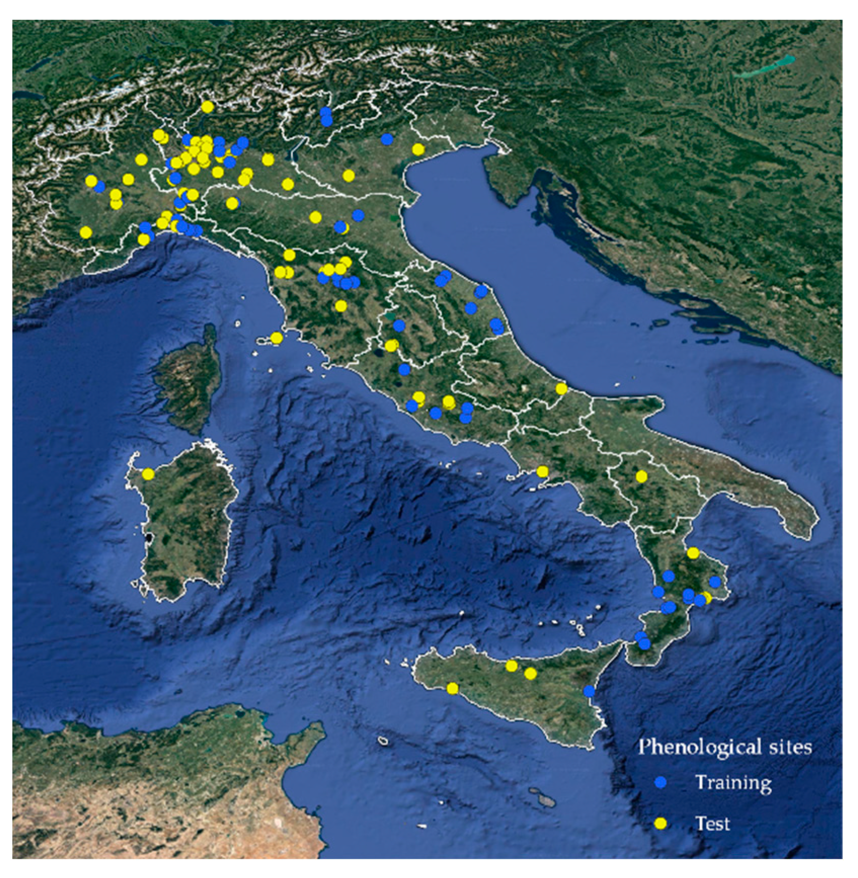
Since 2010, data on black locust (
Robinia pseudoacacia L.) were recorded from weekly surveys carried out at a total of 145 different monitoring sites distributed throughout Italy (
Figure 1), with an elevation range between 0 and 1000 m asl and a latitudinal range between 37.53° and 46.28° N. The spatial distribution of monitoring sites was quite representative of the species distribution in Italy [
57] and covered most of the Italian Regions suited to the production of Acacia honey, as shown in the annual report of the Italian national observatory of honey [
58].
Within the IPHEN framework, the BBCH scale was previously adapted to the species considered, selecting a subset of values. The scale used for black locust is presented in
Table 1. For each site, a sample of 10 plants was observed. The median value of the 10 observations was computed as representative of each survey.
A total number of 1993 surveys were derived, covering a period of 12 years (2010–2021). The length of the site series was highly heterogeneous and varied between 1 and 92 surveys per site.
The quality control of phenological observations was performed according to several criteria, and also took into account some indications in the scientific literature [
59,
60], as specified below:
Validation was performed by assessing values in relation to defined rules, such as consistency of geographical coordinates and monitoring area, consistency of the day of the year (DOY) of the observed event and the time range defined for Italy (e.g., 80–180 for flowering phases), detected phenological stages included in the range of the BBCH scale for the observed species and following a correct temporal sequence;
Reliability refers to the completeness and correctness of the dataset: the observation of multiple phenological stages for the same individual plant on the same date is considered an error;
Plausibility is related to the likely accuracy of values. The control focuses on data that are not expected, which can be better understood through ancillary data. In this case, observers were only suggested to add comments to the surveys, concerning, for example, any relative adverse meteorological conditions or specific events that may have compromised the correct phenological development.
Overall, 0.84% of data were flagged as suspect. All flagged data were checked and corrected (if necessary and possible) or excluded from the analysis.
The analysis focused on the main reproductive stages from
inflorescence of flower buds visible to
end of flowering (BBCH 51–69), which were the most surveyed due to the purposes of phenology monitoring mainly linked to beekeeping.
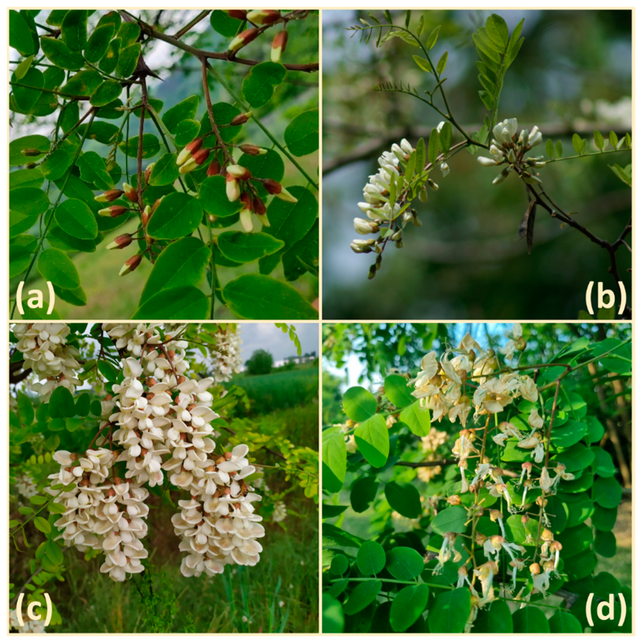
Figure 2 shows some examples of black locust flowering stages. After the quality control, a dataset of 1253 surveys covering these phenological phases (related to 145 sites) was extracted from the database. Only sites with at least two years of observations were considered for the model calibration. Therefore, 64 out of 145 sites were selected for calibration (training set) with a series length ranging from 2 to 11 years. Overall, the training set size was 76% (956 surveys) of the whole dataset, while validation was based on a test set consisting of 297 surveys over 81 sites. The distribution of training and test sites is represented in
Figure 1.
2.2. Meteorological Data
In order to develop a simulation of black locust phenology, each monitoring site must be accompanied by a specific meteorological series in order to analyze the relationships between environmental conditions and plant development.
For this purpose, a gridded dataset of daily maximum and minimum temperature (Italian Temperature Gridded Dataset-ITGD) was obtained by spatial interpolation of the Global Surface Summary of the Day (GSOD-NOAA) dataset for Italy, provided by a maximum number of 157 Italian weather stations per year (
Figure 3), excluding annual series with more than 5% of missing values. In the case of missing data, this data source was integrated with the forecast COSMO-ME (COnsortium for Small-scale MOdelling-Mediterranean-European domain) dataset [
61]. The study area embraces Italy within 35.45 N–47.14 N and 6.56 E–18.58 E.
It is important to highlight that COSMO-ME forecasts are currently used for the periodic publication of the operational cartographic products of IPHEN. The grid base chosen for the air temperature interpolation, at resolution 0.045° Lat/Lon, is the same of COSMO-ME, also to improve prospective overlay with other official datasets. The elevation layer was obtained from three tiles (eu_dem_v11_E40N10, eu_dem_v11_E40N20, eu_dem_v11_E50N10) of the European Digital Surface Model (EU-DEM), version 1.1, at 25m resolution (EPSG:3035, ETRS89-LAEA), made available through the Copernicus Land Monitoring Service (CLMS) [
62]. This derived layer was then resampled to the coarser resolution of COSMO-ME using the bilinear interpolation method.
For validation, daily temperature data for 2006–2015 were used from 81 independent weather stations, belonging to local and national networks, distributed across the Italian territory (
Figure 3). Some more details about test stations are provided in
Table 2.
2.3. Pre-Processing
Using the GSOD dataset, monthly lapse rates of minimum and maximum temperatures in relation to elevation and latitude were estimated based on monthly average measures of 183 stations in the period 1998–2018. Only series with at least 83% of non-missing data per month were included in the analysis. The spatialization was performed in two steps. Firstly, station data were linearly adjusted to sea level using the modeled lapse rates and were spatialized by a local interpolation method (Thin Plate Spline). Then, the final temperature (minimum and maximum) layers were obtained reconstructing the lapse rates using the resampled EU-DEM.
Table 3 reports the mean absolute error (MAE) per elevation range and season, derived from external validation (based on the cited 81 independent stations). Overall, performance results were better for maximum (2.23 °C) than for minimum temperature (2.88 °C). Best performances were obtained at an elevation below 800 m asl and in the winter season, for both variables.
For phenology modeling purposes, complete temperature time series at an hourly time-resolution are needed. Therefore, daily data were extracted from the ITGD at each phenology monitoring site and hourly time series were calculated by the Parton and Logan algorithm [
63].
2.4. Phenology Modeling
The modeling of phenology of black locust, as for all the other species covered by the IPHEN project, is based on the accumulation of active temperatures calculated with the Normal Heat Hour (NHH) method [
7,
21,
64,
65]. This approach tries to overcome the main limitation of the majority of growing degree days-based models, namely the presupposition of a linear relationship between temperature and plant development rate, neglecting the detrimental effects of over-optimal temperatures [
8,
9].
With the NHH approach, the plant rate of development is obtained by weighting hourly temperature with a response function based on four parameters (LC—lower cardinal, LOC—lower optimal cardinal, UOC—upper optimal cardinal, UC—upper cardinal) that translates an hour spent at a given temperature into a Normal Heat Hour. In more detail, hourly temperatures outside the LC—UC range are translated into 0 NHH (null rate of development), while temperatures inside the LOC—UOC range are equal to 1 NHH (maximum rate of development). With temperatures moving from LC to LOC, NHHs linearly increase from 0 to 1, while with temperatures moving from UOC to UC, NHHs linearly decrease from 1 to 0 [
21].
As for most permanent trees phenology modeling, active temperature is usually accumulated from 1 January of each year. The trials showed that start dates play the main role in model performance results, followed by LC. In this study, after a preliminary analysis of the model performance with different sequences of starting dates, firstly ranging from 1 to 75 with a step of 15 and then between 60 and 74 with a step of 5, the analysis focused on the two more promising starting dates: 1 and 10 March.
Table 4 shows 5184 modeling solutions based on the two starting dates and the combination of different values of the four cardinal temperatures were tested for calibration purposes in order to identify the best set of parameters to minimize errors in prediction (the best goodness of fit).
Considering all training sites, for each combination of parameters, every phenological observation was paired with the accumulation of NHH (NHHcum). Hence, the median NNHcum value was assigned to each BBCH stage; then a linear regression was performed between these two variables. For this purpose, only BBCH phases with more than 20 observations were considered (for a total of 896 surveys). Finally, based on the linear regression, simulated BBCH were derived from NHHcum values.
Validation was carried out by running the fitted model on the temperature data of 81 test phenological sites (297 surveys) and deriving performance metrics.
The model performance was assessed by comparing, for every site, the mean DOY for each simulated BBCH phase with the DOY corresponding to the same observed phase. In both calibration and validation, the goodness of fit was assessed by quantitative statistics [
66], including Mean Error (Equation (1)), Mean Absolute Error (Equation (2)), Root Mean Square Error (Equation (3)) and Nash–Sutcliffe Efficiency (Equation (4)) as defined below:
where
Pi and
Oi are the predicted and the observed DOY of each phase emergence.
Data processing for both temperature interpolation and phenology modeling was performed using the open-source software R [
67]. The flowchart presented in
Figure 4 summarizes the overall procedure adopted for modeling the black locust flowering.
3. Results
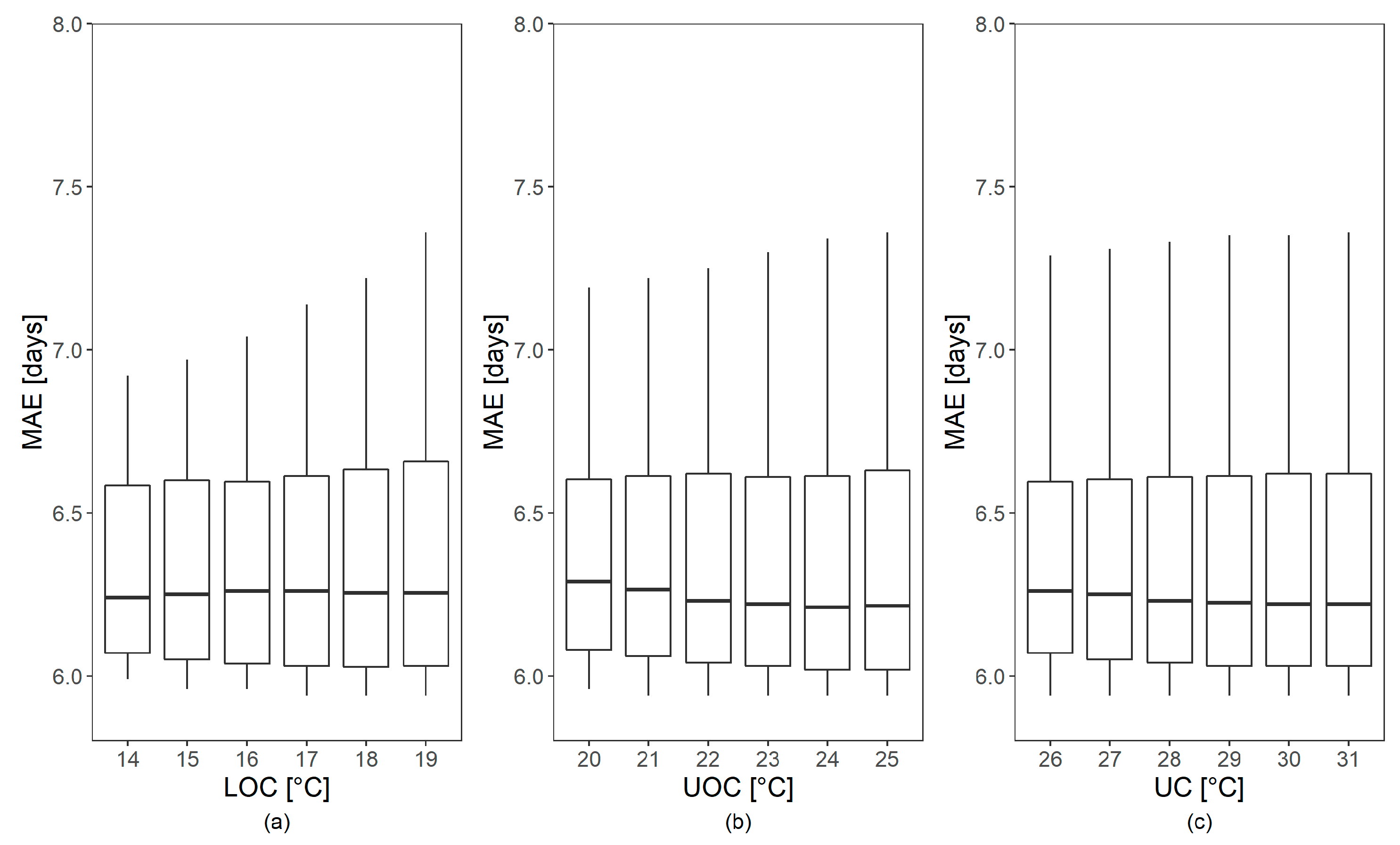
As described in the methods section, a first coarse calibration proposed 1 and 10 March (DOY 60 and 69, respectively) as a putative starting date for NHH accumulation. As shown in
Figure 5 the lowest MAE values were obtained with DOY 69 and an LC value of 1 °C. Overall, performance metrics were highly dependent on LC, while the studied ranges of the other parameters LOC, UOC and UC showed a negligible effect (
Figure 6).
According to the goodness of fit, the optimum model was obtained with the following parameter set: 69, 0, 19, 24, 27 for starting DOY, LC, LOC, UOC, UC, respectively. The regression equation for simulating the BBCH from cumulative NHH values (NHHcum) is presented in
Table 5.
The analysis of calibration results in relation to the main ranges of BBCH flowering phases shows that prediction of pre-flowering phases (51–59) is less precise (highest error dispersion), whereas generally the model overestimates the prediction for early flowering phases (60–64), with a median error of 2.5 days (
Figure 7). The best results in terms of bias are reached in late flowering phases (65–69).
In
Figure 8, the expected dates of the flowering phases (BBCH 51–69) are plotted against those observed for the validation dataset, showing a relatively good correlation, with some outliers, mainly related to the late flowering phases. Generally, most accurate predictions are tied to the central dates of the flowering period.
The main model performance metrics derived from the training and test sets were calculated by geographical area and elevation range, respectively.
At a national level, NSE values higher than 0.7 were reached in calibration as well as in validation, with an MAE value of approximately 6 days. In the test, the model shows a small delay of about 1 day (ME). On average, the model gave the best NSE values for both training (0.77) and test (0.79) sets in the north, characterized by the largest size of surveys. Worse performances were obtained for the test set (NSE equal to 0.32) in the south, where the number of surveys is lowest (
Table 6). It should be noted that in this zone the black locust occurrence is less important than in the rest of Italy, as reported by Rizzo and Gasparini [
57].
With reference to the elevation range, the model showed the best results below 350 m asl, while in the highest altitudinal belt all performance metrics were worse, both in calibration and validation (
Table 7). It should be noted that despite this elevation class being very broad, ranging from 350 to 1000 m asl, and including only 23% of training surveys, MAE values are below 7 for training as well as test sets.
4. Discussion
The temporal and spatial coverage of the IPHEN dataset on black locust phenology allowed the obtaining of quite satisfactory results in calibrating a model for this species at a national scale. The analyses carried out during the calibration process highlighted that prediction performances mostly depend on the choice of the starting date as well as on the first cardinal temperature (LC). With reference to cardinal temperatures, these findings are comparable with those reported by Otero et al. [
68] for cereals, who highlighted that an appropriate base temperature is crucial to thermal time modeling; base temperature may vary between species and even throughout the phenological phases. However, the estimated value often depends on the method used for its determination. In addition, cardinal temperatures vary with the phenological phase, as observed in Oryza sativa by Ellis et al. [
69].
As for black locust, the present analysis focused on modeling the flowering stages at a national scale in Italy, as these are the most represented in the database as beekeepers involved in monitoring are more interested in this target period. Two analogous studies were previously carried out in Italy, based on a more limited set of observations (both in terms of sites and years): the first showed a model based on three cardinals [
7], which were set to 10, 22 and 38 °C, while the second study applied a four-cardinals approach, whose values were close the previous ones: 12, 24, 34 and 38 °C [
51]. Both these studies did not investigate the effect of the starting date on model performances, which was set to the 1st of January. The best cardinal temperatures found in these earlier studies differ greatly from the current results (0, 19, 24 and 27 °C). However, it should be noted that the model presented in this paper also includes the starting DOY among the parameters, whose value (60 or 69) corresponds to the beginning of March, when the mean temperatures are close to the lower cardinal temperatures used by the studies cited (10 or 12 °C).
The RMSE value of 7.98 days for flowering prediction, found for the model validation at a national scale, is aligned with the findings for black locust of Ziegler et al. [
70] (7.81 days) and of Czernecki et al. [
53], who obtained a value of approximately 7 days with models based only on meteorological predictors. Tao et al. [
55] reported higher RMSE values (above 9.7 days) in modeling leaf coloring dates; this worse result confirms the lower sensitivity to temperature of plants during the late phenological stages [
53].
The main result of the present study is an improvement in performance for flowering prediction in Italy compared to Alilla et al. [
51]. At a national scale, the performance on the validation dataset was in fact much better in terms of MAE (6.11 instead of 7.5 days) and NSE (0.71 instead of 0.35). The model showed similar performances also at a sub-national level and within different elevation ranges, with MAE values generally lower than 7 days, and slightly higher for Central Italy. These error values are below the weekly sampling frequency adopted, which is the time scale typical of forest phenology monitoring. In this context, some authors have chosen to directly predict phenological timing in terms of the week of the year (WOY) rather than the day of the year (DOY) [
32,
33].
The best accuracies in prediction were reached in the BBCH range 65–69, which also covers the most important phenological period for beekeepers. In fact, in
R. pseudoacacia the quantity of nectar tends to increase progressively with the advance of the flowering phases and the maximum secretion is reached approximately on the 6th day after the opening of the flowers and continues until the end of flowering (BBCH 69) [
71]. In addition, honeybees are probably more suitable for exploiting ageing flowers rather than applying the force needed to open the petals of a fresh flower to reach the nectars [
72]. It should be noted that the model performances shown in the pre-flowering period (BBCH range 51–59) may provide nomadic beekeepers with useful indications to plan a timely management of beehives.
However, in the analysis of the obtained results, some limitations in the approach followed for the model calibration should be considered, mainly due to the specific characteristics of input data used. First, the uncertainty derived from the interpolation process adopted for meteorological data produces an error propagation which impacts on the final results. On the other hand, despite the efforts made to standardize phenological data collection through training sessions and supervision based on the acquisition of photos, these data are also affected by a not negligible uncertainty due to the subjectiveness of surveyors and to the weekly periodicity of observations. Furthermore, as the collection of data in the field is performed on a voluntary basis, the time series are affected by missing data and are sometimes not homogeneous. As referred to by Ziegler et al. [
70], different estimations of the error generated by observers are reported in the literature and they range from ± 2–3 days to 1–2 weeks.
The present study focused on the relationship between flowering and temperature, while it did not investigate the impact of other major drivers on phenology development, such as precipitation, photoperiod, irradiance, winter chilling, competition, resource limitations and genetics [
19]. Spano et al. [
44] reported that the first flowering dates are highly correlated with temperature (growing degree days) in
Robinia pseudoacacia and did not highlight any significant effect of rainfall and drought on flowering. Similar results were obtained by Szabò et al. [
48], who found a good relationship between temperature and flowering, while precipitation correlation was not significant.
Another aspect to be considered is the genetic variability of the sampled trees, due to their spontaneous regeneration. Even though black locust is not a native species in the study area, it has been present in the Italian area for a long time. This implies a further variability source in the flowering dates. Nevertheless, the specific survey protocol adopted, which requires the observation of 10 plants per site, may lead to reduce this variability and make the different samples more comparable. The same considerations apply to the different sunlight conditions of the single trees, as the survey protocol includes specific guidelines for choosing plants in ordinary conditions, in terms of geomorphology and vegetation.
Finally, it should be highlighted that other main drivers can affect phenology, such as physiological processes typical of each species, which are not completely understood and therefore are currently not considered by process-based phenology models [
6]; moreover, the role of biotic interactions with the phenology has been little investigated [
73].
5. Conclusions
The study results have shown that the calibration provided good results in terms of precision and accuracy. For this reason, the new version of the black locust phenological model will be adopted next season in the context of IPHEN activities.
The model presented is simple and easy to apply; therefore, it lends itself to operational use in specific services including phenological monitoring and forecasting maps for Italy. These maps can allow the comparison of past climate phases with future climate scenarios, assessing the impact of climate change in the flowering timing of the plant.
Further developments will concern the analysis of relationships between phenology and climate change in relation to other Italian native species occurring in the same ecological niche (i.e., chestnut, which is also monitored within the IPHEN project), in view of the definition of adaptation strategies for the honey production sector. In fact, nomadic beekeepers can benefit from these analyses for planning their future activities in the framework of climate changes.


