
Assessment of Land Consolidation Processes from an Environmental Approach: Considerations Related to the Type of Intervention and the Structure of Farms

 , ,
, ,
Abstract
:1. Introduction
2. Materials and Methods
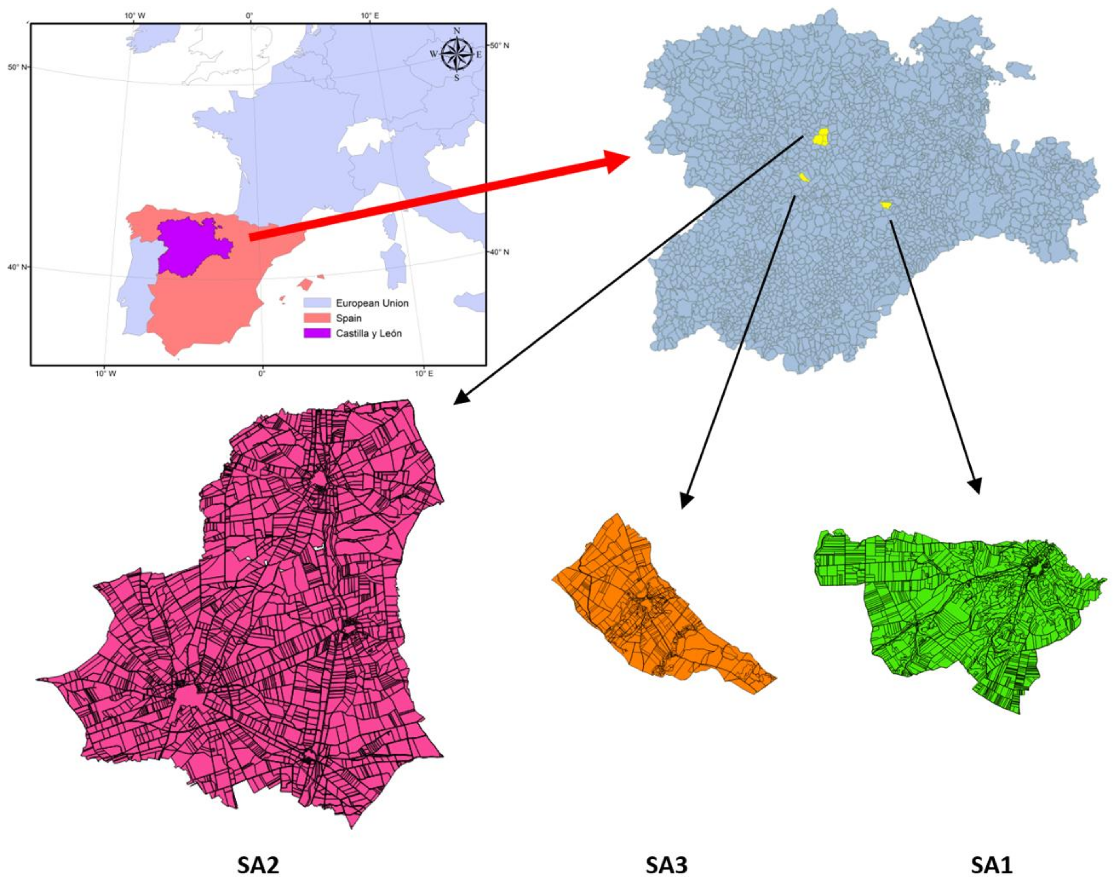
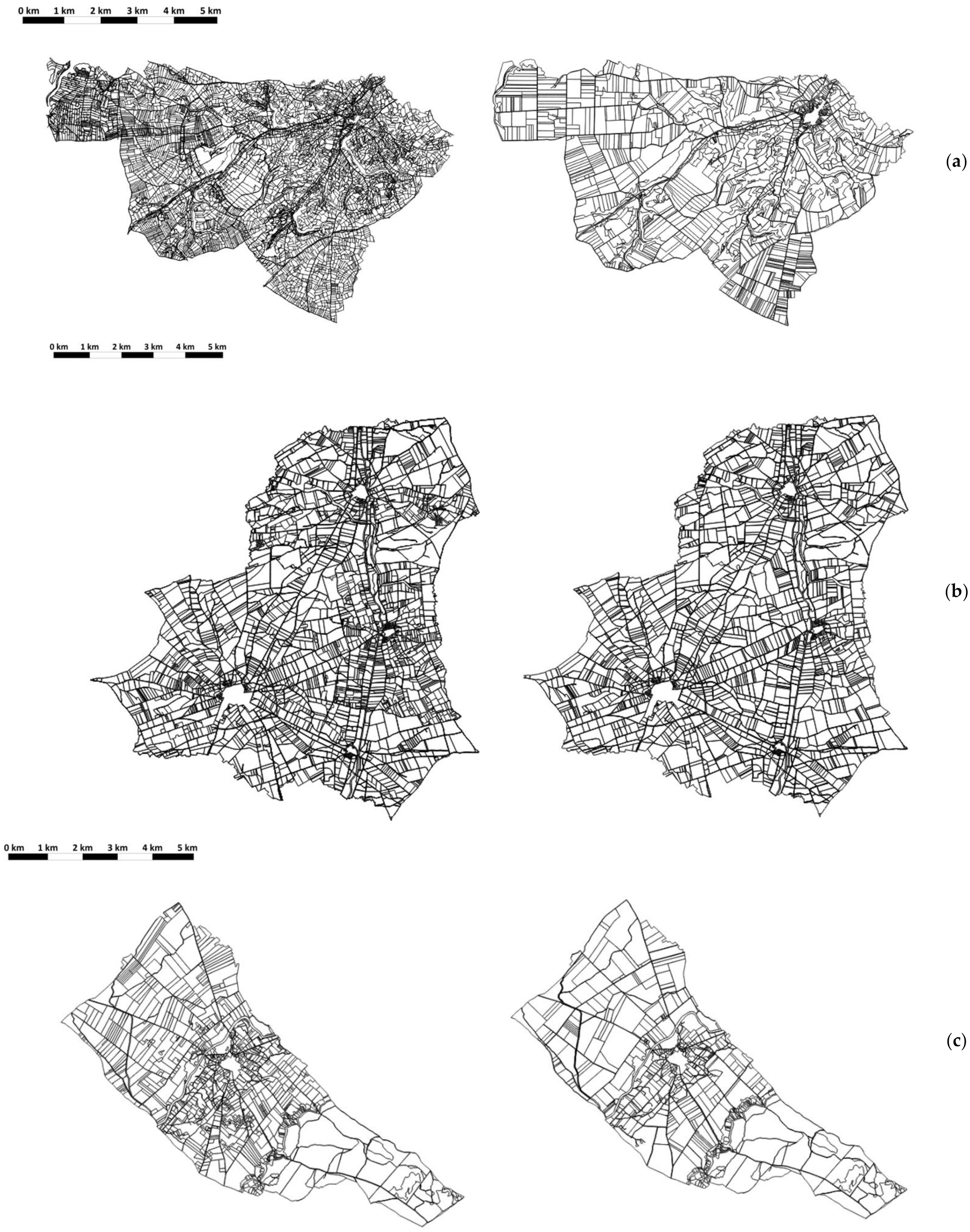
2.1. Study Areas
- SA1 is the first LCP. It is located in a single municipal area with non-irrigated crops (>95% crop area),
- SA2 is the second LCP affecting four municipal areas with non-irrigated farming (>99% crop area),
- SA3 is an LCP in a single municipal area with non-irrigated and irrigated areas (ratio 2/1).
- Non-consolidated areas versus areas with a first LCP: SA1 vs. SA2 and SA3;
- The boundaries of the project involve various municipal areas or a single village: SA2 vs. SA1 and SA3;
- Significant presence or lack of irrigated crops in the LC area: SA3 vs. SA1 and SA2.
2.2. Databases
2.3. Election of the Study Sample
2.4. Software Used
2.5. Design and Calculation Criteria
2.5.1. Spatial Organization
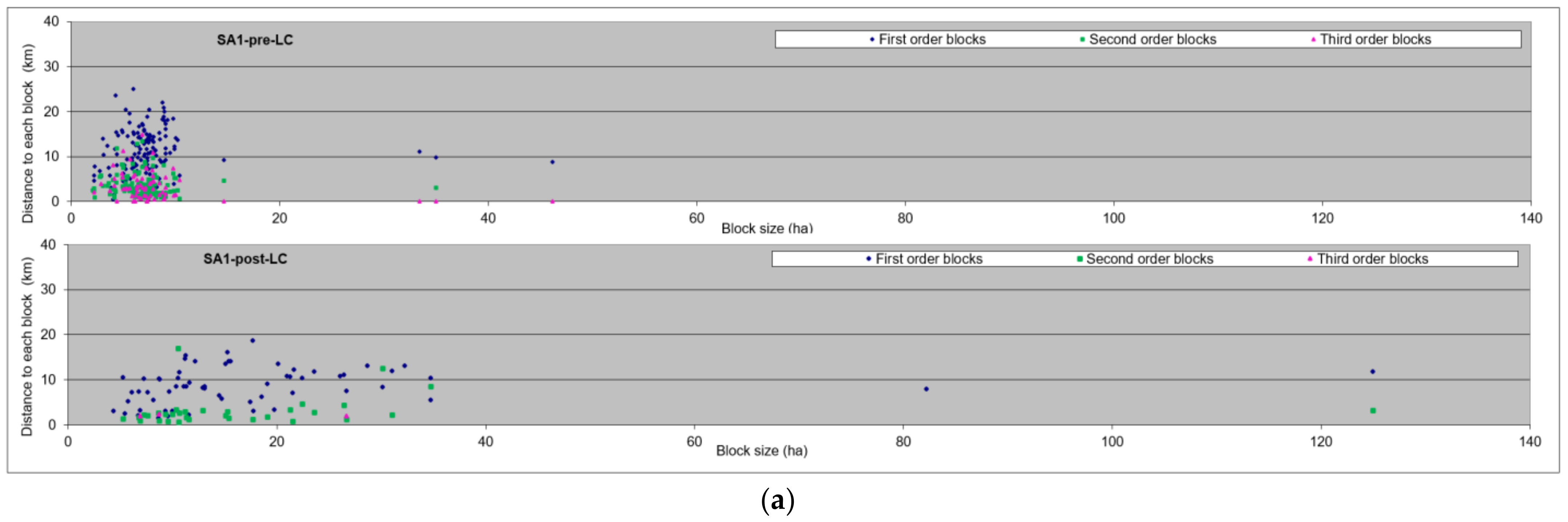
2.5.2. Calculations Linked to the Journeys to Each Block
2.5.3. Calculation Linked to Row-End Turnings in Each Block
3. Results
3.1. Adjustment of the Size of the Block According to Their Geometric Regularity
3.2. Fuel Consumption Linked to the Itineraries of Each Block
3.3. Consumption Linked to Row-End Turnings in Each Block
4. Discussion
4.1. Adjustment of the Size of the Blocks According to the Geometric Regularity
4.2. Variation of the Fuel Consumption According to the Journeys to Each Block
4.3. Variations of the Fuel Consumption Considering the Turning Operations within Each Block
5. Conclusions
- generation of new restructuring of the plots,
- land consolidation of irrigation plots,
- creation of LC areas taking various municipal areas,
- consideration of the plots based outside of the LC perimeter.
Author Contributions
Funding
Institutional Review Board Statement
Informed Consent Statement
Data Availability Statement
Acknowledgments
Conflicts of Interest
Appendix A

| Farming Operations | Features Implement/Machine | C (h/ha) 1 | % Use 2 | CR 3 | CUS 4 | ||||||
|---|---|---|---|---|---|---|---|---|---|---|---|
| CH 5 | CF 6 | OR 7 | |||||||||
| CH 5 | CF 6 | OR 7 | 0.82 | 0.15 | 0.03 | ||||||
| Primary tillage | 1 | 1 | 1 | 0.86 | 0.16 | 0.03 | |||||
| Mouldboard or disc plough | 4 c–14″ | 1.42 m | 25 cm | 1.18 | 0.1 | ||||||
| Mouldboard or disc plough | 3 c–16″ | 1.22 m | 32 cm | 2 | 0.2 | ||||||
| Chisel plough | 2.0 m | 18 cm | 1.2 | 0.3 | |||||||
| Heavy cultivator | 3.0 m | 18 cm | 0.44 | 0.4 | |||||||
| Secondary ploughing 1 | 2 | 2 | 2 | 1.47 | 0.27 | 0.05 | |||||
| Disc harrow | 4.5 m | 15 cm | 0.37 | 0.1 | |||||||
| Cultivator | 2.5 m | 15 cm | 1.1 | 0.5 | |||||||
| Power harrow | 3.0 m | 15 cm | 0.78 | 0.4 | |||||||
| Secondary ploughing 2 | 1 | 1 | 1 | 0.37 | 0.07 | 0.01 | |||||
| Roller | 5.0 m | 300 kg/m | 0.31 | 0.3 | |||||||
| Roller | 3.0 m | 300 kg/m | 0.52 | 0.7 | |||||||
| Sowing | 1 | 0.5 | 1 | 0.71 | 0.06 | 0.03 | |||||
| SC + R 8 | 5.0 m | boot | 0.91 | 0.8 | |||||||
| Direct seeding | 3.0 m | disc | 0.69 | 0.2 | |||||||
| Chemical fertilisation | 1 | 3 | 4 | 0.15 | 0.08 | 0.02 | |||||
| Suspended fertiliser spreader | 1 disc | 12.0 m | 650 L | 0.21 | 0.06 | ||||||
| Suspended fertiliser spreader | 1 disc | 16.0 m | 800 L | 0.13 | 0.2 | ||||||
| Large hopper fertiliser spreader | 2 discs | 24.0 m | 1400 L | 0.08 | 0.2 | ||||||
| Organic fertilisation | 0.33 | 0.1 | 0.67 | 0.27 | 0.01 | 0.02 | |||||
| Manure distributor | 4 t | 3.20 m | 1.05 | 0.9 | |||||||
| Slurry distribution tank | 5 m3 | 7.00 m | 0.51 | 0.1 | |||||||
| Crop protection | 0.6 | 2 | 3 | 0.3 | 0.11 | 0.04 | |||||
| PBS 9 | 16 m | 1200 L | 0.13 | 0.3 | 0.2 | ||||||
| PBS 9 | 6 m | 400 L | 0.54 | 0.6 | 0.2 | ||||||
| PBA 10 | 24 m | 3000 L | 0.08 | 0.1 | |||||||
| Recolection MAT 11 | 0 | 4 | 0.4 | 0 | 1.19 | 0.02 | |||||
| Mower | discs | 2.50 m | tdf 15 | 0.82 | 0.8 | ||||||
| RHA 12 | pinwheel | 8.00 m | t df 15 | 0.2 | 0.8 | ||||||
| Classic baler | heavy | 2.00 m | 5 t/h | 1.17 | 0.8 | ||||||
| Round baler-E 13 | 10 t/h | 5.00 m | 1 | 0.1 | |||||||
| Macro baler | 20 t/h | 6.00 m | 0.37 | 0.1 | |||||||
| Self-loading wagon | 35 m3 | 5.00 m | 0.48 | 0.2 | |||||||
| Recolection MAP 14 | 1 | 0 | 0.6 | 0.31 | 0 | 0.01 | |||||
| Harvester | 6 m | 1000 h | 3 t/ha | 0.39 | 0.7 | ||||||
| Harvester | 7 m | 1000 h | 5 t/ha | 0.34 | 0.3 | ||||||
| Average 9 farming operations | 0.56 | 0.24 | 0.03 | ||||||||
| Average mean yield (h/ha) | 0.83 | ||||||||||
Appendix B
| Farming Operation | Itinerary | Energy |
|---|---|---|
| Deep ploughing | single | light |
| Deep ploughing | return | heavy |
| Cultivator + roller | round trip | light |
| Fertilization (autumn) | single | heavy |
| Fertilization (autumn) | return | light |
| Harrow + roller | round trip | light |
| Sowing | round trip | light |
| Phytosanitary treatment (fungi) | round trip | light |
| Phytosanitary treatment (insects) | round trip | light |
| Fertilization (spring) | single | heavy |
| Fertilization (spring) | return | light |
| Mulching | single | heavy |
| Mulching | return | light |
| Forage mowing | round trip | light |
| Forage tedding and swathing | round trip | light |
| Forage baling | round trip | light |
| Installation of irrigation equipment | round trip | light |
| De-installation of irrigation equipment | round trip | light |
References
- United Nations Framework Convention for Climate Change. Paris Agreement; Climate Change Secretariat: Bonn, Germany, 2015. [Google Scholar]
- Intergovernmental Panel on Climate Change. Climate Change 2013: The Physical Science Basis. Contribution of Working Group I to the Fifth Assessment Report of the Intergovernmental Panel on Climate Change; Stocker, T.F., Qin, D., Plattner, G.K., Tignor, M., Allen, S.K., Boschung, J., Nauels, A., Xia, Y., Bex, V., Midgley, P.M., Eds.; Cambridge University Press: Cambridge, UK, 2013. [Google Scholar]
- UN Climate Change Secretariat. Annual Report 2021. Annex I Party GHG Inventory Submissions. Available online: https://unfccc.int/es/node/210513 (accessed on 17 September 2021).
- Johnson, J.M.-F.; Franzluebbers, A.J.; Lachnicht Weyers, S.; Reicosky, D.C. Agricultural opportunities to mitigate greenhouse gas emissions. Environ. Pollut. 2007, 150, 107–124. [Google Scholar] [CrossRef] [PubMed]
- Hillier, J.; Walter, C.; Malin, D.; Garcia-Suarez, T.; Mila-i-Canals, L.; Smith, P. A farm-focused calculator for emissions from crop and livestock production. Environ. Model. Softw. 2011, 26, 1070–1078. [Google Scholar] [CrossRef]
- Povellato, A.; Bosello, F.; Giupponi, C. Cost-effectiveness of greenhouse gases mitigation measures in the European agro-forestry sector: A literature survey. Environ. Sci. Policy 2007, 10, 474–490. [Google Scholar] [CrossRef]
- Smith, P.; Martino, D.; Cai, Z.; Gwary, D.; Janzen, H.; Kumar, P.; McCarl, B.; Ogle, S.; O’Mara, F.; Rice, C.; et al. Policy and technological constraints to implementation of greenhouse gas mitigation options in agriculture. Agric. Ecosyst. Environ. 2007, 118, 6–28. [Google Scholar] [CrossRef]
- Sanz-Cobena, A.; Lassaletta, L.; Aguilera, E.; del Prado, A.; Garnier, J.; Billen, G.; Iglesias, A.; Sanchez, B.; Guardia, G.; Abalos, D. Strategies for greenhouse gas emissions mitigation in Mediterranean agriculture: A review. Agric. Ecosyst. Environ. 2017, 238, 5–24. [Google Scholar] [CrossRef] [Green Version]
- Vergé, X.P.C.; De Kimpe, C.; Desjardins, R.L. Agricultural production, greenhouse gas emissions and mitigation potential. Agric. For. Meteorol. 2007, 142, 255–269. [Google Scholar] [CrossRef]
- Schneider, U.A.; McCarl, B.A.; Schmid, E. Agricultural sector analysis on greenhouse gas mitigation in US agriculture and forestry. Agric. Syst. 2007, 94, 128–140. [Google Scholar] [CrossRef]
- Dyer, J.A.; Kulshreshtha, S.N.; McConkey, B.G.; Desjardins, R.L. An assessment of fossil fuel energy use and CO2 emissions from farm field operations using a regional level crop and land use database for Canada. Energy 2010, 35, 2261–2269. [Google Scholar] [CrossRef]
- Dalgaard, T.; Olesen, J.E.; Petersen, S.O.; Petersen, B.M.; Jørgensen, U.; Kristensen, T.; Hutchings, N.J.; Gyldenkærne, S.; Hermansen, J.E. Developments in greenhouse gas emissions and net energy use in Danish agriculture–How to achieve substantial CO2 reductions? Environ. Pollut. 2011, 159, 3193–3203. [Google Scholar] [CrossRef]
- Fellmann, T.; Pérez Domínguez, I.; Witzke, P.; Weiss, F.; Hristov, J.; Barreiro-Hurle, J.; Leip, A.; Himics, M. Greenhouse gas mitigation technologies in agriculture: Regional circumstances and interactions determine cost-effectiveness. J. Clean. Prod. 2021, 317, 128406. [Google Scholar] [CrossRef]
- Pervanchon, F.; Bockstaller, c.; Girardin, P. Assessment of energy use in arable farming systems by means of an agro-ecological indicator: The energy indicator. Agric. Syst. 2002, 72, 149–172. [Google Scholar] [CrossRef]
- Lacour, S.; Langle, T.; Dieudé-Fauvel, É. Déterminer l’impact environnemental de la consommation de carburant des tracteurs agricoles: Simulation et comparaison. Sci. Eaux Territ. 2011, 1, 74–81. [Google Scholar] [CrossRef]
- Shamshiri, R.; Ehsani, R.; Maja, J.M.; Roka, F.M. Determining machine efficiency parameters for a citrus canopy shaker using yield monitor data. Appl. Eng. Agric. 2013, 29, 33–41. [Google Scholar] [CrossRef] [Green Version]
- Zegada-Lizarazu, W.; Matteucci, D.; Monti, A. Critical review on energy balance of agricultural systems. Biofuels Bioprod. Biorefining 2010, 4, 423–446. [Google Scholar] [CrossRef]
- Hercher-Pasteur, J.; Loiseau, E.; Sinfort, C.; Hélias, A. Energetic assessment of the agricultural production system. A review. Agron. Sustain. Dev. 2020, 40, 29. [Google Scholar] [CrossRef]
- Nielsen, V.; Luoma, T. Energy consumption: Overview of data foundation and extract of results. In Agricultural Data for Life Cycle Assessments; Weidema, B.P., Meeusen, M.J.G., Eds.; Agricultural Economics Research Institute (LEI): The Hague, The Netherlands, 2000; Volume 1, pp. 51–69. [Google Scholar]
- Voltr, V.; Hruška, M.; Nobilis, L. Complex Valuation of Energy from Agricultural Crops including Local Conditions. Energies 2021, 14, 1415. [Google Scholar] [CrossRef]
- Hiironen, J.; Riekkinen, K. Agricultural impacts and profitability of land consolidations. Land Use Policy 2016, 55, 309–317. [Google Scholar] [CrossRef]
- González, X.P.; Marey, M.F.; Álvavez, C.J. Evaluation of productive rural land patterns with joint regard to the size, shape and dispersion of plots. Agric. Syst. 2007, 92, 52–62. [Google Scholar] [CrossRef]
- EU Council. Regulation (EU) 2018/841 of the European Parliament and of the Council of 30 May 2018 on the Inclusion of Greenhouse Gas Emissions and Removals from Land Use, Land Use Change and Forestry in the 2030 Climate and Energy Framework and Amending Regulation (EU) No 525/2013 and Decision No 529/2013/EU; EU Council: Brussels, Belgium, 2018. [Google Scholar]
- De Cara, S.; Jayet, P.A. Marginal abatement costs of greenhouse gas emissions from European agriculture, cost effectiveness, and the EU non-ETS burden sharing agreement. Ecol. Econ. 2011, 70, 1680–1690. [Google Scholar] [CrossRef] [Green Version]
- Crecente, R.; Álvarez, C. Una revisión de la concentración parcelaria en Europa. Estud. Agrosoc. Y Pesq. 2000, 187, 221–274. [Google Scholar] [CrossRef]
- Crecente, R.; Álvarez, C.; Fra, U. Economic, social and environmental impact of land consolidation in Galicia. Land Use Policy 2002, 19, 135–147. [Google Scholar] [CrossRef]
- González, X.P.; Álvarez, C.J.; Crecente, R. Evaluation of land distributions with joint regional to plot, size and shape. Agric. Syst. 2004, 82, 31–43. [Google Scholar] [CrossRef]
- Shan, W.; Xiaobin, J.; Xuhong, Y.; Zhengming, G.; Bo, H.; Hanbing, L.; Yinkang, Z. A framework for assessing carbon effect of land consolidation with life cycle assessment: A case study in China. J. Environ. Manag. 2020, 266, 110557. [Google Scholar] [CrossRef]
- Comunidad de Castilla y León. Ley 14/1990, de 28 de noviembre, de Concentración Parcelaria de Castilla y León. BOCyL nº 241, de 14 de diciembre de 1990. Boletín Of. Del Estado 1991, 28, 3556–3566. [Google Scholar]
- Comunidad de Castilla y León. Ley 1/2014, de 19 de marzo, Agraria de Castilla y León. Libro segundo, Título II. BOCyL nº 55, de 20 de marzo de 2014. Boletín Of. Del Estado 2014, 250, 87210. [Google Scholar]
- Ramírez del Palacio, Ó.J. Contribución del Proceso de Concentración Parcelaria a la Reducción de Las Emisiones de Gases de Efecto Invernadero: Estudio de Dos Casos en La Estepa Cerealista de Castilla y León (España). Master’s Thesis, Escuela Técnica Superior de Ingenierías Agrarias, Universidad de Valladolid, Valladolid, Spain, 2011; p. 28. Available online: https://uvadoc.uva.es/browse?authority=7f214a06-4b15-40de-9385-eeecd42131d2&type=author (accessed on 20 November 2021).
- Servicio de Ordenación de Explotaciones. Situación de la Concentración Parcelaria en Castilla y León. Memoria 2017; Dirección General de Producción Agropecuaria e Infraestructuras Agrarias, Consejería de Agricultura y Ganadería, Junta de Castilla y León: Valladolid, España, 2017. [Google Scholar]
- Van Dijk, T. Complications for traditional land consolidation in Central Europe. Geoforum 2007, 38, 505–511. [Google Scholar] [CrossRef]
- Akkaya Aslan, S.T.; Gundogdu, K.S.; Yaslioglu, E.; Kirmikil, M.; Arici, I. Personal, physical and socioeconomic factors affecting farmers’ adoption of land consolidation. Span. J. Agric. Res. 2007, 5, 204–213. [Google Scholar] [CrossRef] [Green Version]
- Wu, Z.; Liu, M.; Davis, J. Land consolidation and productivity in Chinese household crop production. China Econ. Rev. 2005, 16, 28–49. [Google Scholar] [CrossRef]
- Hiironen, J.; Niukkanen, K. On the structural development of arable land in Finland–How costly will it be for the climate? Land Use Policy 2014, 36, 192–198. [Google Scholar] [CrossRef]
- Tan, S.; Heerink, N.; Kruseman, G.; Qu, F. Do fragmented landholdings have higher production costs? Evidence from rice farmers in Northeastern Jiangxi province, P.R. China. China Econ. Rev. 2008, 19, 347–358. [Google Scholar] [CrossRef]
- Harasimowicz, S.; Janus, J.; Bacior, S.; Gniadek, J. Shape and size of parcels and transport costs as a mixed integer programming problem in optimization of land consolidation. Comput. Electron. Agric. 2017, 140, 113–122. [Google Scholar] [CrossRef]
- Demetriou, D. The assessment of land valuation in land consolidation schemes: The need for a new land valuation framework. Land Use Policy 2016, 58, 487–498. [Google Scholar] [CrossRef]
- Zhang, Z.; Zhao, W.; Gu, X. Changes resulting from a land consolidation project (LCP) and its resource–environment effects: A case study in Tianmen City of Hubei Province, China. Land Use Policy 2014, 40, 74–82. [Google Scholar] [CrossRef]
- Sklenicka, P. Applying evaluation criteria for the land consolidation effect to three contrasting study areas in the Czech Republic. Land Use Policy 2006, 23, 502–510. [Google Scholar] [CrossRef]
- Kolis, K.; Hiironen, J.; Riekkinen, K.; Vitikainen, A. Forest land consolidation and its effect on climate. Land Use Policy 2017, 61, 536–542. [Google Scholar] [CrossRef]
- Zhang, X.; Ye, Y.; Wang, M.; Yu, Z.; Luo, J. The micro administrative mechanism of land reallocation in land consolidation: A perspective from collective action. Land Use Policy 2018, 70, 547–558. [Google Scholar] [CrossRef]
- Cay, T.; Iscan, F. Fuzzy expert system for land reallocation in land consolidation. Expert Syst. Appl. 2011, 38, 11055–11071. [Google Scholar] [CrossRef]
- Demetriou, D. Automating the land valuation process carried out in land consolidation schemes. Land Use Policy 2018, 75, 21–32. [Google Scholar] [CrossRef]
- Kik, R. A method for reallotment research in land development projects in The Netherlands. Agric. Syst. 1990, 33, 127–138. [Google Scholar] [CrossRef]
- Harasimowicz, S.; Bacior, S.; Gniadek, J.; Ertunç, E.; Janus, J. The impact of the variability of parameters related to transport costs and parcel shape on land reallocation results. Comput. Electron. Agric. 2021, 185, 106137. [Google Scholar] [CrossRef]
- Xanthoulis, D.; Fleussu, B. Etude d’impact du Remembrement sur l’environement. Partie II. Aspects Energetiques; Office Wallon du Développement Rural–Faculté des Sciences Agronomiques de Gembloux: Gembloux, Belgium, 1995; total pages 30. [Google Scholar]
- Wu, Y.; Zhou, Y.; Guo, Y.; Wang, L. The energy emission computing of land consolidation from the dual perspectives clustering method. Clust. Comput. 2017, 20, 979–987. [Google Scholar] [CrossRef]
- Instituto Nacional de Estadística. Censo Agrario 2009. Retrieved 11-12-2019, from Instituto Nacional de Estadística. Ministerio de Asuntos Económicos y Transformación Digital. Available online: https://www.ine.es/CA/Inicio.do (accessed on 20 November 2021).
- Servicio de Estadística, Secretaría General de la Consejería de Agricultura, Ganadería y Desarrollo Rural. Anuario de Estadística Agraria de Castilla y León. Varios años; Servicio de Estadística, Secretaría General de la Consejería de Agricultura, Ganadería y Desarrollo Rural, Junta de Castilla y León: Valladolid, España, 2020; Available online: https://agriculturaganaderia.jcyl.es/web/jcyl/AgriculturaGanaderia/es/Plantilla100/1284228463984/_/_/_ (accessed on 20 November 2021).
- EU. Regulation (EU) No 1307/2013 of the European Parliament and of the Council of 17 December 2013 Establishing Rules for Direct Payments to Farmers under Support Schemes within the Framework of the Common Agricultural Policy and Repealing Council Regulation (EC) No 637/2008 and Council Regulation (EC) No 73/2009, DOUE No 347 12-20-2013; European Commision-EU: Brussels, Belgium, 2013. [Google Scholar]
- QGIS Development Team. QGIS Geographic Information System; 2.18.5; QGIS: Zurich, Switzerland, 2015. [Google Scholar]
- Autodesk. Autocad 2016; Autodesk, Inc.: San Rafael, CA, USA, 2016. [Google Scholar]
- Del Río Salio, M. RouteGEN; Universidad de Valladolid-ETSIT, Departamento de Teoría de la Señal y Comunicaciones e Ingeniería Telemática: Valladolid, Spain, 2005. [Google Scholar]
- SAS, version 9.4; SAS Institute: Cary, NC, USA, 2021.
- EU-Commission. Annual European Union Greenhouse Gas Inventory 1990–2018 and Inventory Report. 2020. Available online: https://www.eea.europa.eu/publications/european-union-greenhouse-gas-inventory-2020 (accessed on 20 November 2021).
- Agencia Europea del Medio Ambiente, AEMA. Europe´s Environment, The Four Assessment; AEMA: Copenhagen, Denmark, 2007. [Google Scholar]
- Huang, W.H. Optimal line-sweep-based decompositions for coverage algorithms. In Proceedings of the IEEE International Conference on Robotics and Automation, Seoul, Korea, 21–26 May 2001; Volume 1, pp. 27–32. [Google Scholar]
- Oksanen, T. Path Planning Algorithms for Agricultural Machine. Ph.D. Thesis, Helsinki University of Technology, Espoo, Finland, 2007. [Google Scholar]
- Francart, C.; Pivot, J.-M. Incidences de la structure parcellaire sur le fonctionnement des exploitations agricoles en régions de bocage. Ingénieries-EAT 1998, 14, 41–54. Available online: https://hal.archives-ouvertes.fr/hal-00461165 (accessed on 1 March 2021).
- Rodias, E.; Berruto, R.; Busato, P.; Bochtis, D.; Sørensen, C.G.; Zhou, K. Energy savings from optimised in-field route planning for agricultural machinery. Sustainability 2017, 9, 1956. [Google Scholar] [CrossRef] [Green Version]
- Cadastral Database, Secretaría de Estado de Hacienda. Dirección General del Catastro. Ministerio de Hacienda y Administraciones Públicas. 2019. Available online: https://www.sedecatastro.gob.es/Accesos/SECAccDescargaDatos.aspx (accessed on 20 July 2021).
- Boto Fidalgo, J.A.; Pastrana Santamarta, P.; Suárez de Cepeda Martínez, M. Consumos Energéticos en Las Operaciones Agrícolas en España; Instituto para la Diversificación y Ahorro de la Energía, IDEA–MITECO: Madrid, Spain, 2005. [Google Scholar]
- Dyer, J.A.; Desjardins, R.L. Simulated Farm Fieldwork, Energy Consumption and Related Greenhouse Gas Emissions in Canada. Biosyst. Eng. 2003, 85, 503–513. [Google Scholar] [CrossRef]
- Marie, M. Des Pratiques des Agriculteurs à la Production de Paysage de Bocage. Étude Comparée des Dynamiques et des Logiques D’organisation Spatiale des Systèmes Agricoles Laitiers en Europe (Basse-Normandie, Galice, Sud de l’Angleterre). Ph.D. Thesis, Université de Caen, Caen, France, 2009; p. 514. [Google Scholar]
- Instituto para la Diversificación y Ahorro de la Energía. Ahorro, Eficiencia Energética y Estructura de la Explotación Agrícola. Serie “Ahorro y Eficiencia Energética en la Agricultura”; IDEA–MITECO: Madrid, Spain, 2006. [Google Scholar]
- Bochtis, D.D.; Vougioukas, S.G. Minimising the non-working distance travelled by machines operating in a headland field pattern. Biosyst. Eng. 2008, 101, 1–12. [Google Scholar] [CrossRef]
- Janulevičius, A.; Šarauskis, E.; Čiplienė, A.; Juostas, A. Estimation of farm tractor performance as a function of time efficiency during ploughing in fields of different sizes. Biosyst. Eng. 2019, 179, 80–93. [Google Scholar] [CrossRef]
- Koniuszy, A.; Kostencki, P.; Berger, A.; Golimowski, W. Power performance of farm tractor in field operations. Eksploat. I Niezawodn. Maint. Reliab. 2017, 19, 43–47. [Google Scholar] [CrossRef]
- Lovarelli, D.; Bacenetti, J.; Fiala, M. Effect of local conditions and machinery characteristics on the environmental impacts of primary soil tillage. J. Clean. Prod. 2017, 140, 479–491. [Google Scholar] [CrossRef]
- He, P.; Li, J.; Fang, E.; deVoil, P.; Cao, G. Reducing agricultural fuel consumption by minimizing inefficiencies. J. Clean. Prod. 2019, 236, 17619. [Google Scholar] [CrossRef]
- Hameed, I.A.; Bochtis, D.D.; Sørensen, C.G.; Nøremark, M. Automated generation of guidance lines for operational field planning. Biosyst. Eng. 2010, 107, 294–306. [Google Scholar] [CrossRef]
- Latruffe, L.; Piet, L. Does land fragmentation affect farm performance? A case study from Brittany, France. Agric. Syst. 2014, 129, 68–80. [Google Scholar] [CrossRef]
- Gniadek, J.; Harasimowicz, S.; Janus, J.; Pijanowski, J.M. Optimization of the parcel layout in relation to their average distance from farming settlements in the example of Mściwojów village, Poland. Geomat. Landmanagement Landsc. 2013, 2, 25–35. [Google Scholar] [CrossRef]
- Grammatikopoulou, I.; Myyrä, S.; Pouta, E. The proximity of a field plot and land-use choice: Implications for land consolidation. J. Land Use Sci. 2013, 8, 383–402. [Google Scholar] [CrossRef] [Green Version]
- Zhu, Y.; Waqas, M.A.; Li, Y.; Zou, X.; Jiang, D.; Wilkes, A.; Qin, X.; Gao, Q.; Wan, Y.; Hasbagan, G. Large-scale farming operations are win-win for grain production, soil carbon storage and mitigation of greenhouse gases. J. Clean. Prod. 2018, 172, 2143–2152. [Google Scholar] [CrossRef]
- Yan, M.; Cheng, K.; Luo, T.; Yan, Y.; Pan, G.X.; Rees, R.M. Carbon footprint of grain crop production in China–based on farm survey data. J. Clean. Prod. 2015, 104, 130–138. [Google Scholar] [CrossRef]
- Pishgar-Komleh, S.H.; Ghanderijani, M.; Sefeedpari, P. Energy consumption and CO2, emissions analysis of potato production based on different farm size levels in Iran. J. Clean. Prod. 2012, 33, 183–191. [Google Scholar] [CrossRef]
- Bernhardt, H.; Götz, S.; Heizinger, V.; Zimmermann, N.; Engelhardt, D. Energy consumption of agricultural transports and influencing factors. In Proceedings of the International Conference of Agricultural Engineering CIGR-AgEng, Valencia, Spain, 8–12 July 2012; Volume 8, p. 12. [Google Scholar]
- Lacour, S.; Burgun, C.; Perilhon, C.; Descombes, G.; Doyen, V. A model to assess tractor operational efficiency from bench test data. J. Terramechanics 2014, 54, 1–18. [Google Scholar] [CrossRef]
- Auernhammer, H. Precision farming-the environmental challenge. Comput. Electron. Agric. 2001, 30, 31–43. [Google Scholar] [CrossRef]
- Lu, H.; Xie, H.; He, Y.; Wu, Z.; Zhang, X. Assessing the impacts of land fragmentation and plot size on yields and costs: A translog production model and cost function approach. Agric. Syst. 2018, 161, 81–88. [Google Scholar] [CrossRef]
- Coletta, A. Impatto della Struttura Fondiaria Sull’efficienza Aziendale. Ph.D. Thesis, Economia Montana e Forestale, Università degli Sudi di Trento, Trento, Italy, 2000; p. 136. [Google Scholar]
- Lorencowicz, E.; Uziak, J. Fuel consumption in family farms. Teka Kom. Motoryz. Energetyki Rol. 2009, 9, 164–171. [Google Scholar]
- Spain–Rural Development Programme (Regional)–Castilla y León. Available online: https://agriculturaganaderia.jcyl.es/web/es/desarrollo-rural/programa-desarrollo-rural-castilla-leon.html (accessed on 1 April 2021).
- MAGRAMA. Cálculo de los Costes de Utilización de Aperos y Máquinas Agrícolas. 2014. Available online: https://www.mapa.gob.es/es/ministerio/servicios/informacion/plataforma-de-conocimiento-para-el-medio-rural-y-pesquero/observatorio-de-tecnologias-probadas/maquinaria-agricola/costes-aperos-maquinas.aspx (accessed on 10 May 2021).


| SA1 | SA2 | SA3 | |
|---|---|---|---|
| Period of execution 1st LC | 2007–2010 | 1968–1975 | 1963–1967 |
| Period of execution 2nd LC | - | 2004–2009 | 2008–2011 |
| Work execution period | 2017–2019 | 2010–2015 | 2015–2017 |
| LCP surface (ha) | 4254.75 | 16,056.03 | 2715.46 |
| Owners (n) | 581 | 1258 | 245 |
| Plots Ex ante-LC (n) | 5676 | 4759 | 1111 |
| Plots per owner Ex ante-LC (n) | 9.77 | 3.78 | 4.53 |
| Mean size of the plots Ex ante-LC (ha) | 0.71 | 3.36 | 2.43 |
| Plots Ex post-LC (n) | 1068 | 2157 | 482 |
| Plots per owner Ex post-LC (n) | 1.84 | 1.71 | 1.97 |
| Mean size of the plots Ex post-LC (ha) | 3.77 | 7.42 | 5.52 |
| RI 1 | 5.31 | 2.21 | 2.30 |
| LCI 2 | 0.90 | 0.74 | 0.73 |
| SA1 | SA2 | SA3 | ||||
|---|---|---|---|---|---|---|
| Pre-LC | Post-LC | Pre-LC | Post-LC | Pre-LC | Post-LC | |
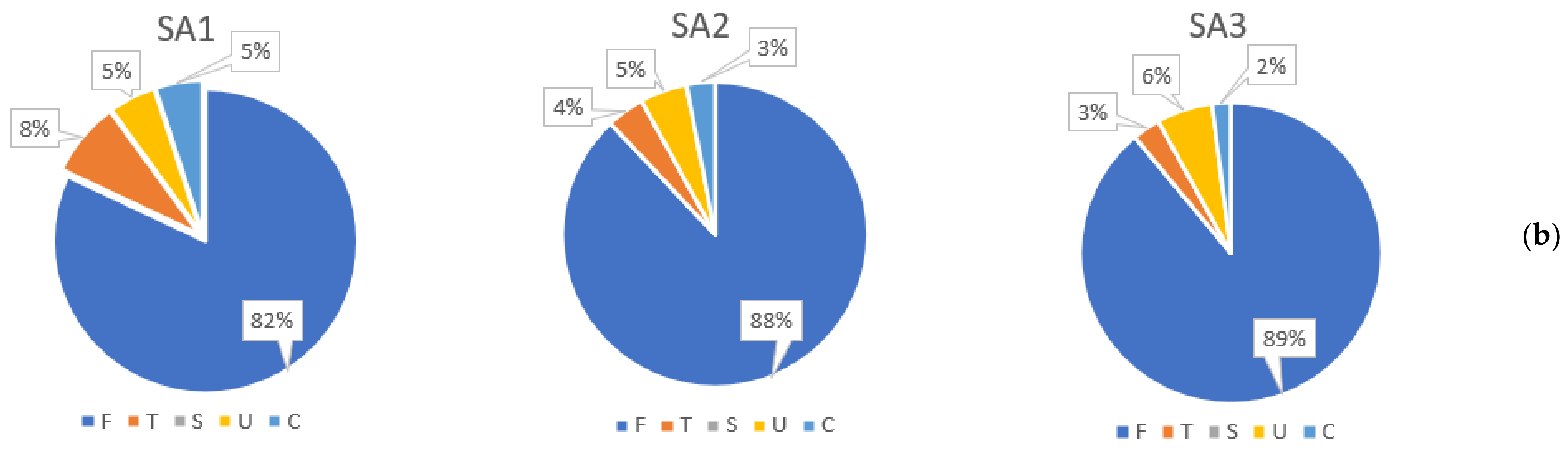
| Exploitations (n) | 24 | 41 | 19 | |||
| Exploitations (%) 1 | 43.64 | 33.34 | 48.72 | |||
| Exploitations < 30 ha (n) | 4 | 26 | 7 | |||
| Exploitations 30.01–50 ha (n) | 12 | 2 | 5 | |||
| Exploitations 50.01–100 ha (n) | 5 | 5 | 4 | |||
| Exploitations 100.01–200 ha (n) | 3 | 7 | 2 | |||
| Exploitations > 200.01 ha (n) | 0 | 1 | 1 | |||
| Exploitation surface (ha) | 1069.77 | 1059.31 | 1804.25 | 1934.60 | 1034.02 | 1018.27 |
| Exploitation surface (%) 2 | 26.51 | 26.25 | 11.36 | 12.18 | 38.33 | 37.75 |
| Plots (n) | 1384 | 204 | 548 | 205 | 403 | 151 |
| Plots (%) 3 | 24.38 | 19.10 | 11.52 | 9.50 | 36.27 | 31.33 |
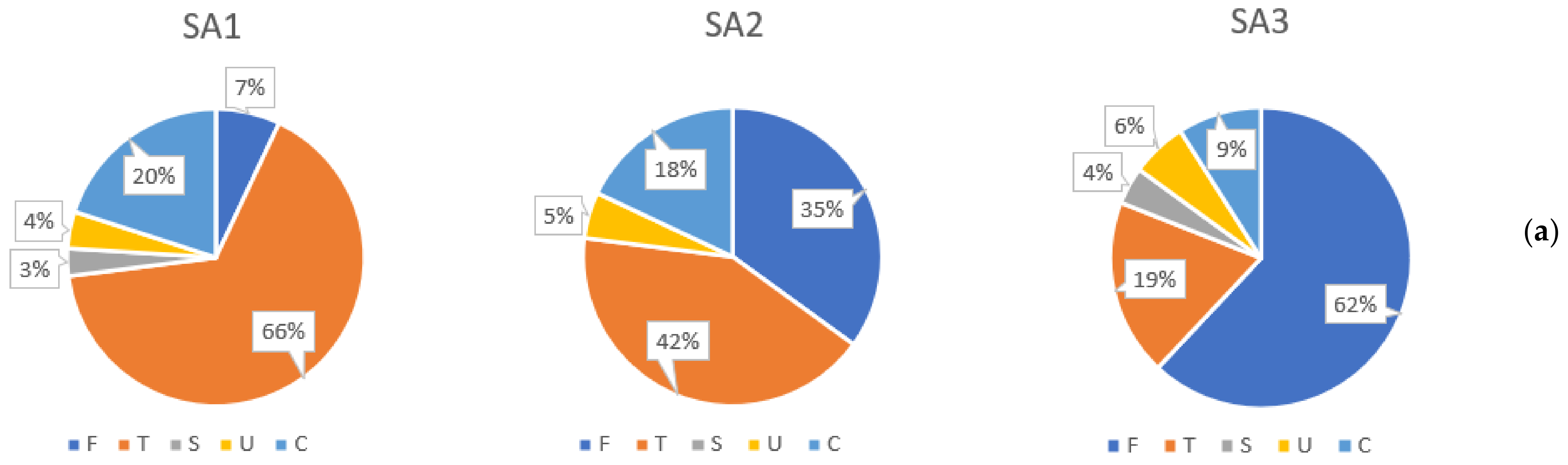
| Regular (%) | Irregular (%) | Highly Irregular (%) | ||||
|---|---|---|---|---|---|---|
| Pre-LC | Post-LC | Pre-LC | Post-LC | Pre-LC | Post-LC | |
| SA1 | 39.71 | 51.00 | 49.29 | 42.00 | 11.00 | 7.00 |
| SA2 | 27.52 | 24.24 | 43.12 | 61.62 | 29.36 | 14.14 |
| SA3 | 16.00 | 27.03 | 53.60 | 62.16 | 30.40 | 10.81 |
| LCP | n 1 | Mean Surface and Standard Deviation of the Exploitation (ha) | Mean Surface and Standard Deviation of the Block (ha) | |||
|---|---|---|---|---|---|---|
| Pre-LC | Post-LC | Pre-LC | Post-LC | |||
| SA1 | T 2 | 24 | 44.60 ± 31.13 | 44.14 ± 31.26 | 6.86 ± 2.07 | 16.09 ± 8.25 |
| V 3 | 3 | 19.56 ± 20.12 | 17.45 ± 18.50 | 5.88 ± 1.38 | 8.84 ± 3.80 | |
| SA2 | T 2 | 41 | 44.01 ± 57.29 | 47.19 ± 58.83 | 9.48 ± 5.90 | 18.73 ± 20.05 |
| V 3 | 16 | 44.65 ± 68.60 | 46.37 ± 66.23 | 7.22 ± 4.37 | 18.92 ± 20.29 | |
| E 4 | 8 | 73.08 ± 85.88 | 76.46 ± 80.25 | 9.40 ± 4.32 | 27.14 ± 22.89 | |
| SA3 | T 2 | 19 | 54.09 ± 54.56 | 53.76 ± 53.97 | 9.79 ± 4.74 | 18.77 ± 12.86 |
| V 3 | 5 | 21.91 ± 19.53 | 21.33 ± 18.89 | 9.17 ± 3.97 | 16.53 ± 17.19 | |
| S 5 | 14 | 45.83 ± 51.19 | 45.91 ± 51.65 | 10.36 ± 5.27 | 17.20 ± 12.33 | |
| R 6 | 5 | 77.22 ± 63.04 | 75.73 ± 60.14 | 8.17 ± 2.53 | 23.17 ± 14.76 | |
| LCP | n 1 | Distance Covered (km·Block−1) | Variation (%) | Distance Covered (km·ha−1) | Variation (%) | |||
|---|---|---|---|---|---|---|---|---|
| Pre-LC | Post-LC | Pre-LC | Post-LC | |||||
| SA1 | T 2 | 24 | 441.14 ± 106.82 | 326.70 ± 153.00 | −25.94 | 68.81 ± 24.55 | 22.04 ± 11.46 | −67.97 ** |
| V 3 | 3 | 369.45 ± 69.09 | 128.59 ± 63.06 | −65.19 | 66.95 ± 26.34 | 14.23 ± 3.21 | −78.75 | |
| SA2 | T 2 | 41 | 313.98 ± 171.30 | 235.40 ± 155.72 | −25.03 | 53.07 ± 60.93 | 30.64 ± 60.06 | −42.26 ** |
| V 3 | 16 | 341.47 ± 247.17 | 224.52 ± 174.60 | −34.25 | 56.75 ± 47.63 | 18.19 ± 13.90 | −67.95 | |
| E 4 | 8 | 488.38 ± 234.96% | 343.85 ± 140.47 | −29.59 | 69.51 ± 60.32 | 16.50 ± 6.55 | −76.26 | |
| SA3 | T 2 | 19 | 307.45 ± 101.46 | 367.72 ± 199.74 | 19.60 | 34.75 ± 18.92 | 22.04 ± 10.51 | −36.58 ** |
| V 3 | 5 | 254.93 ± 176.10 | 274.69 ± 205.60 | 7.75 | 25.39 ± 14.57 | 18.41 ± 14.56 | −27.49 | |
| S 5 | 14 | 298.72 ± 113.48 | 318.77 ± 159.92 | 6.71 | 30.20 ± 11.15 | 21.17 ± 11.06 | −29.90 | |
| R 6 | 5 | 331.88 ± 58.50 | 504.78 ± 254.06 | 52.10 | 47.50 ± 30.53 | 24.45 ± 6.12 | −48.53 | |
| LCP | n 1 | Total Journeys (km·Block−1) | Variation (%) | Total Journeys (km·ha−1) | Variation (%) | ||
|---|---|---|---|---|---|---|---|
| Pre-LC | Post-LC | Pre-LC | Post-LC | ||||
| Exploitations < 25 ha | |||||||
| SA1 | 5 | 498.19 ± 208.54 | 250.93 ± 260.57 | −49.63 | 95.48 ± 40.63 | 26.01 ± 23.28 | −72.75 |
| SA2 | 25 | 327.97 ± 204.47 | 181.44 ± 106.69 | −44.68 | 70.95 ± 70.70% | 42.95 ± 74.79 | −39.47 |
| SA3 | 7 | 274.75 ± 150.69 | 238.62 ± 139.19 | −13.15 | 38.89 ± 30.44 | 26.51 ± 13.90 | −31.83 |
| SA3-S | 5 | 245.14 ± 166.76 | 220.74 ± 161.21 | −9.65 | 27.26 ± 14.74 | 24.83 ± 16.52 | −8.91 |
| SA3-R | 2 | 348.77 ± 98.32 | 283.33 ± 81.73 | −17.33 | 67.97 ± 48.16 | 30.73 ± 4.22 | −54.79 |
| Exploitations 25–50 ha | |||||||
| SA1 | 12 | 435.05 ± 72.44 | 348.82 ± 118.47 | −19.82 | 64.44 ± 8.07 | 23.25 ± 5.30 | −65.52 |
| SA2 | 3 | 358.88 ± 151.22% | 261.30 ± 136.80 | −27.19 | 24.46 ± 10.55 | 17.09 ± 4.83 | −30.14 |
| SA3 | 5 | 328.07 ± 64.46 | 350.04 ± 105.16 | 6.70 | 35.21 ± 9.74 | 20.74 ± 11.78 | −41.10 |
| SA3-S | 5 | 328.07 ± 64.46 | 350.04 ± 105.16 | 6.70 | 35.21 ± 9.74 | 20.74 ± 11.78 | −41.10 |
| SA3-R | 0 | N/A | N/A | N/A | N/A | N/A | |
| Exploitations 50–100 ha | |||||||
| SA1 | 4 | 405.64 ± 45.19 | 342.95 ± 102.20 | −15.45 | 60.02 ± 5.06 | 21.55 ± 3.58 | −64.09 |
| SA2 | 6 | 268.88 ± 79.19 | 220.95 ± 74.52 | −17.83 | 21.41 ± 7.43 | 11.36 ± 4.77 | −46.95 |
| SA3 | 4 | 296.45 ± 43.84 | 337.33 ± 70.14 | 14.80 | 32.58 ± 2.45 | 18.22 ± 2.94 | −44.08 |
| SA3-S | 3 | 305.58 ± 46.21 | 312.82 ± 61.42 | 2.37 | 25.99 ± 10.86 | 17.45 ± 3.07 | −32.86 |
| SA3-R | 1 | 291.55 | 410.88 | 40.93 | 36.09 | 20.54 | −43.09 |
| Exploitations 100–150 ha | |||||||
| SA1 | 3 | 417.74 ± 24.63 | 342.86 ± 149.54 | −17.93 | 41.59 ± 13.27 | 11.22 ± 5.50 | −73.02 |
| SA2 | 2 | 301.85 ± 108.16 | 655.01 ± 288.42 | 117.00 | 18.08 ± 10.09 | 10.01 ± 2.46 | −44.64 |
| SA3 | 2 | 335.15 ± 44.09 | 773.17 ± 23.22 | 130.69 | 32.72 ± 1.72 | 20.14 ± 0.64 | −38.44 |
| SA3-S | 0 | N/A | N/A | N/A | N/A | N/A | |
| SA3-R | 2 | 335.15 ± 44.09 | 773.17 ± 23.22 | 130.69 | 32.72 ± 1.72 | 20.14 ± 0.64 | −38.44 |
| Exploitations > 150 ha | |||||||
| SA1 | 0 | N/A | N/A | N/A− | N/A | N/A | |
| SA2 | 5 | 245.08 ± 30.83 | 261.94 ± 30.13 | 6.88 | 19.78 ± 2.17 | 8.93 ± 2.0 pre2 | −54.83 |
| SA3 | 1 | 421.87 | 670.45 | 58.92 | 23.45 | 16.28 | −30.58 |
| SA3-S | 1 | 421.87 | 670.45 | 58.92 | 23.45 | 16.28 | −30.58 |
| SA3-R | 0 | N/A | N/A | N/A | N/A | N/A | |
| LCP | n 1 | Consumption Per Journey to Each Block (L·ha−1) | ||
|---|---|---|---|---|
| Pre-LC | Post-LC | |||
| SA1 | T 2 | 24 | 32.81 ± 12.75 | 8.42 ± 3.91 ** |
| V 3 | 3 | 35.27 ± 12.74 | 5.46 ± 0.75 | |
| SA2 | T 2 | 41 | 23.92 ± 27.31 | 10.96 ± 20,44 ** |
| V 3 | 16 | 24.48 ± 22.14 | 6.69 ± 4.80 | |
| E 4 | 8 | 29.98 ± 29.60 | 6.45 ± 2.36 | |
| SA3 | T 2 | 19 | 16.19 ± 7.07 | 6.41 ± 2.74 ** |
| V 3 | 5 | 13.22 ± 7.18 | 5.48 ± 3.91 | |
| S 5 | 14 | 14.65 ± 4.86 | 6.09 ± 3.12 | |
| R 6 | 5 | 20.53 ± 10.79 | 7.31 ± 0.96 | |
| LCP | n 1 | Consumption According to the Geometric Regularity (L·ha−1) | Consumption According to the Size of the Block (L·ha−1) | |||
|---|---|---|---|---|---|---|
| Pre-LC | Post-LC | Pre-LC | Post-LC | |||
| SA1 | T 2 | 24 | 4.17 ± 0.37 | 3.80 ± 0.94 * | 7.17 ± 1.38 | 2.59 ± 0.54 ** |
| V 3 | 3 | 4.26 ± 0.22 | 2.65 ± 1.07 | 7.64 ± 0.96 | 2.91 ± 0.48 | |
| SA2 | T 2 | 41 | 3.78 ± 1.08 | 3.35 ± 1.54 ns | 4.38 ± 2.17 | 2.86 ± 1.99 ** |
| V 3 | 16 | 3.95 ± 1.10 | 3.93 ± 1.46 | 4.71 ± 2.56 | 3.19 ± 2.74 | |
| E 4 | 8 | 4,04 ± 1.30 | 4.02 ± 1.17 | 3.33 ± 0.83 | 2.27 ± 0.82 | |
| SA3 | T 2 | 19 | 4.21 ± 1.56 | 3.72 ± 1.69 ns | 5.00 ± 2.87 | 2.80 ± 1.13 ** |
| V 3 | 5 | 3.7 ± 0.88 | 4.34 ± 1.75 | 3.50 ± 0.85 | 2.67 ± 0.66 | |
| S 5 | 14 | 3.64 ± 1.20 | 3.60 ± 1.09 | 4.18 ± 0.96 | 2.66 ± 0.87 | |
| R 6 | 5 | 5.82 ± 1.34 | 4.06 ± 0.85 | 7.30 ± 5.00 | 3.18 ± 1.74 | |
Publisher’s Note: MDPI stays neutral with regard to jurisdictional claims in published maps and institutional affiliations. |
© 2022 by the authors. Licensee MDPI, Basel, Switzerland. This article is an open access article distributed under the terms and conditions of the Creative Commons Attribution (CC BY) license (https://creativecommons.org/licenses/by/4.0/).
Share and Cite
Ramírez del Palacio, Ó.; Hernández-Navarro, S.; Sánchez-Sastre, L.F.; Fernández-Coppel, I.A.; Pando-Fernández, V. Assessment of Land Consolidation Processes from an Environmental Approach: Considerations Related to the Type of Intervention and the Structure of Farms. Agronomy 2022, 12, 1424. https://doi.org/10.3390/agronomy12061424
Ramírez del Palacio Ó, Hernández-Navarro S, Sánchez-Sastre LF, Fernández-Coppel IA, Pando-Fernández V. Assessment of Land Consolidation Processes from an Environmental Approach: Considerations Related to the Type of Intervention and the Structure of Farms. Agronomy. 2022; 12(6):1424. https://doi.org/10.3390/agronomy12061424
Chicago/Turabian StyleRamírez del Palacio, Óscar, Salvador Hernández-Navarro, Luis Fernando Sánchez-Sastre, Ignacio Alonso Fernández-Coppel, and Valentín Pando-Fernández. 2022. "Assessment of Land Consolidation Processes from an Environmental Approach: Considerations Related to the Type of Intervention and the Structure of Farms" Agronomy 12, no. 6: 1424. https://doi.org/10.3390/agronomy12061424