Development of Pedotransfer Functions to Predict Soil Physical Properties in Southern Quebec (Canada)

Abstract

Pedotransfer functions (PTFs) are empirical fits to soil property data and have been used as an alternative tool to in situ measurements for estimating soil hydraulic properties for the last few decades. PTFs of Saxton and Rawls, 2006 (PTFs’S&R.2006) are some of the most widely used because of their global aspect. However, empirical functions yield more accurate results when trained locally. This study proposes a set of agricultural PTFs developed for southern Quebec, Canada for three horizons (A, B, and C). Four response variables (bulk density (ρ_b), saturated hydraulic conductivity (K_sat), volumetric water content at field capacity (θ₃₃), and permanent wilting point (θ₁₅₀₀)) and four predictors (clay, silt, organic carbon, and coarse fragment percentages) were used in this modeling process. The new PTFs were trained using the stepwise forward regression (SFR) and canonical correlation analysis (CCA) algorithms. The CCA- and SFR-PTFs were in most cases more accurate. Θ₁₅₀₀ and at θ₃₃ estimates were improved with the SFR. The ρ_b in the A horizon was moderately estimated by the PTFs’S&R.2006, while the CCA- and SFR-PTFs performed equally well for the B and C horizons, yet qualified weak. However, for all PTFs for all horizons, K_sat estimates were unacceptable. Estimation of ρ_b and K_sat could be improved by considering other morphological predictors (soil structure, drainage information, etc.).

1. Introduction

A thorough knowledge of soil physical properties is important for crop production, water resource management, erosion risk prevention, contaminant discharge, and flooding interventions. Measurement of soil physical properties such as porosity and saturated hydraulic conductivity can be expensive and time-consuming. In order to avoid laborious measurements, Pedotransfer functions (PTFs) are used as predictors to estimate the physical characteristics of soil by using soil properties that are abundant, easy to measure, and inexpensive. PTFs are frequently developed to estimate volumetric water content for any given matric potential, porosity, saturated hydraulic conductivity, or bulk density. PTFs are also used to estimate plant available water [1,2], to model physical properties of soil during seasonal evapotranspiration [3], or to characterize the parameters of water retention curve models [4,5]. The most common predictors of soil physical properties are soil particle size distribution, organic matter content, coarse fragment content, and sometimes bulk density. Some authors also used texture class [6], moisture class [7], and soil morphological data such as soil structure [8] and color [9].

According to Patil and Singh [10], there exist two methods of PTF development: mechanistic and empirical approaches. Mechanistic approaches translate easily measured soil properties such as texture, bulk density, and particle density into an equivalent pore size distribution model. This model is then related to water content at different soil matric heads. The physico-empirical model of Arya, et al. [11] is one of the most popular mechanistic approaches. Empirical approaches, on the other hand, fit a correlation function between the predictor and response variables. Two empirical approaches are commonly used: statistical regressions [12,13,14] and data mining and exploration techniques [15,16,17,18]. Data mining and exploration techniques include, among others, regression trees [19,20], artificial neural networks [21,22], and group methods of data handling [23,24]. The results of empirical approach-based PTFs can take the form of a numeric value or a characteristic class. Most PTFs, however, are developed for a given local or regional pedoclimatic context and are, therefore, site-specific and not universally transferable [25].

As an alternative solution, global datasets have been used in previous studies instead of local or regional datasets, in which case the authors included pedoclimatic predictors such as temperature and moisture [26,27]. For example, the PTFs developed by Saxton and Rawls [28] (referred to here as PTFs’S&R.2006) include soil water characteristic equations formed from the US Department of Agriculture soil database using the available soil texture and organic matter variables. In fact, this is an update of the PTFs developed by Saxton et al. [29], including more variables and a wider range of application. They have been combined with previously reported relationships for stresses and conductivities and the effects of density, gravel, and salinity to form a comprehensive system for predicting soil water characteristics for agricultural water management and hydrologic analyses. Hence, they are popular and commonly used in soil microclimate modeling [30,31]. PTFs’S&R.2006 are very useful. However, since PTFs are empirical-based algorithms, improved modeling of pedoclimatic predictors could be achieved by using locally trained PTFs [32].

In southern Quebec, PTFs have already been developed to predict organic carbon accumulation in the forest zone [33]. However, no PTFs are currently designed for the agricultural area of southern Quebec. The aim of our study was to develop a new set of PTFs (bulk density, saturated hydraulic conductivity, and volumetric water content measured at two matric potentials: −33 kPa (field capacity) and −1500 kPa (permanent wilting point)) that are well adapted to the pedoclimatic conditions of the agricultural area of southern Quebec. Two statistical methods were tested for deriving PTFs: stepwise forward regression and canonical correlation analysis. The estimation efficiency of this new set of PTFs was then compared with the existing PTFs developed by Saxton and Rawls (2006). Accuracy was assessed using the cross-validation technique from which the R², Nash–Sutcliffe efficiency (NSE) index, root-mean-square error (RMSE), and bias were generated.

2. Materials and Methods

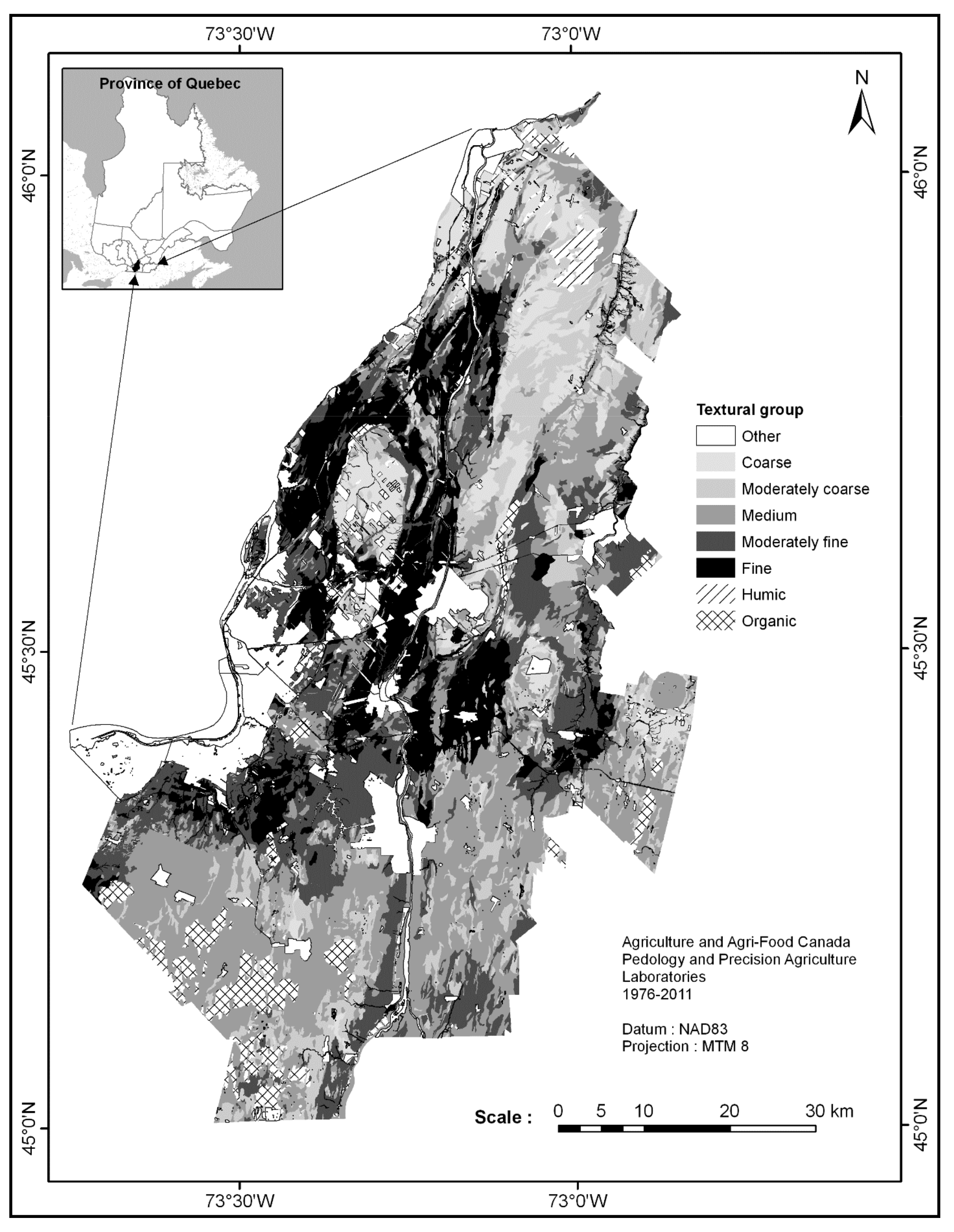
2.1. Study Area

The study was conducted in the Monteregie agricultural area, located southeast of Montréal, Quebec, Canada. The climate of this region is temperate, with an average air temperature of −10.2 °C in January and 20.4 °C in July [34]. In terms of yearly averages, the duration of the frost-free period is 206.5 days, total rainfall is 931.7 mm, and total snowfall is 224.5 cm. Monteregie is one of the largest and most productive agricultural areas in Quebec [35]. Analyses conducted on both ground and surface water using bacteriological and physicochemical indices revealed that water quality is poor at many sampling points [36]. Soil quality was also affected by nutrient leaching, erosion, and overfertilization [37]. Greater use of beneficial management practices is, therefore, needed to ensure soil and water conservation in this region. Development of a set of appropriate PTFs to estimate secondary soil properties would be helpful for planning beneficial management practices implementation.

A high degree of pedodiversity and soil texture variability is perceived in the study area (Figure 1). The soils in this region are gravelly, sandy, loamy, clayey, and organic soils [38]. Many soil taxonomic orders (as defined by the US system of soil taxonomy) are present, including spodosols, inceptisols, and histosols [39]. The soils of the region tend to have poor natural drainage; however, after artificial drainage, they become mostly moderately well drained [40]. Several soil surveys of southern Quebec have been updated since 1975 and are available on the Canadian Soil Information Service website [41].

2.2. Soil Data

Agriculture and Agri-Food Canada (AAFC) has maintained an analytical soil database for southern Quebec since 1975. This database contains a set of georeferenced samples from A, B, and C horizons. Soil physical data (primary and secondary properties) from the analytical soil database were used to develop and assess the proposed PTFs.

Primary soil properties are the first and second components of particle size distribution, such as clay, silt, organic carbon (OC), and coarse fragment (CF) percentages. These properties, which define soil pore space, have an impact on soil water-holding properties, hydraulic conductivity, and soil bulk density. That is why they were chosen as PTF predictors. To avoid multicollinearity problems, sand percentage was not considered. This choice implies the exclusion of organic soils, since they have no mineral content. Soil texture (clay and silt) was determined by the hydrometer method [42], CF (>2 mm) content was determined by sieving [42], and OC content was determined by the Walkley–Black method [43].

Selected secondary soil properties—bulk density (ρ_b), saturated hydraulic conductivity (K_sat), and volumetric water content (θ) measured at two matric potentials, −33 kPa (field capacity (θ₃₃)) and −1500 kPa (permanent wilting point (θ₁₅₀₀))—were considered as response variables in the PTFs. The procedures used to measure θ, ρ_b, and K_sat were described by Topp et al. [44], Culley [45], and Reynolds [46], respectively. The number of samples available for θ₃₃, θ₁₅₀₀, ρ_b, and K_sat was 328, 327, 352, and 310, respectively. These numbers exclude soils that were entirely defined by primary properties and organic soils.

2.3. Statistical Methods

For a given soil profile, the distribution of soil properties changes with depth. For instance, OC tends to decrease with increasing depth [47]. In this paper, most of the studied soils are tilled, which can also influence physical properties (ρ_b, θ, and K_sat) of the A horizon [48]. Consequently, a PTF solely based on A horizon properties is not suitable to estimate soil physical properties at other depths. The dataset used for PTF development in this paper was stratified according to soil horizons (A, B, and C).

Before developing new PTFs, a preliminary study of predictors and response variables is essential [49]. This preliminary study was conducted on each soil dataset corresponding to a soil horizon. The first step was outlier detection. Values larger than three standard deviations from the mean value were regarded outliers and removed from the dataset. Two development approaches were tested: one based on stepwise forward regression (SFR) and the other based on canonical correlation analysis (CCA). The CCA method requires that each soil sample contains all four predictors (clay, silt, OC, and CF) along with the four response variables (θ₁₅₀₀, θ₃₃, ρ_b, and K_sat). To be consistent in both CCA and SFR development methods, only the soil samples having these four predictors and four response variables were kept. In statistical regressions, predictors and response variables must be normally distributed. In order to respect the normality hypothesis, some variables were transformed using the Box–Cox algorithm. The Box–Cox applies a power transformation λ, which maximizes a log-likelihood function (Equation (1)). When the value of λ is 1, a logarithm transformation is applied (Equation (2)).

$$\frac{x^{\lambda }-1}{\lambda },\lambda \ne 0.$$

(1)

$$\ln \left(x\right),\lambda =1.$$

(2)

A correlation study was performed on both predictors and response variables. A strong correlation between predictors indicates that the information is redundant. Adding highly correlated predictors to a PTF will not improve its prediction potential. By contrast, a strong correlation between a predictor and a response variable indicates that selection of the predictor will improve the PTF. Correlation between response variables indicates the linearity of these secondary soil properties.

2.3.1. Stepwise Forward Regression (SFR)

SFR is a commonly used method in statistical regression to identify the most significant predictors when estimating a response variable. The selection of predictors is based on entrance and exit thresholds, which are set according to the p-value of regression coefficients. The p-value is computed to decide whether a given input variable should be considered as a predictor or not. This p-value must be lower than the entrance significance threshold; otherwise, the predictor is rejected. Each time a new predictor is accepted in the regression, the p-values of all previously accepted predictors are recomputed; predictors are retained only if their new values are lower than the exit threshold. Significance levels are fixed at 5% for entrance and exit from the regression model. The method is applied to each response variable using the training dataset.

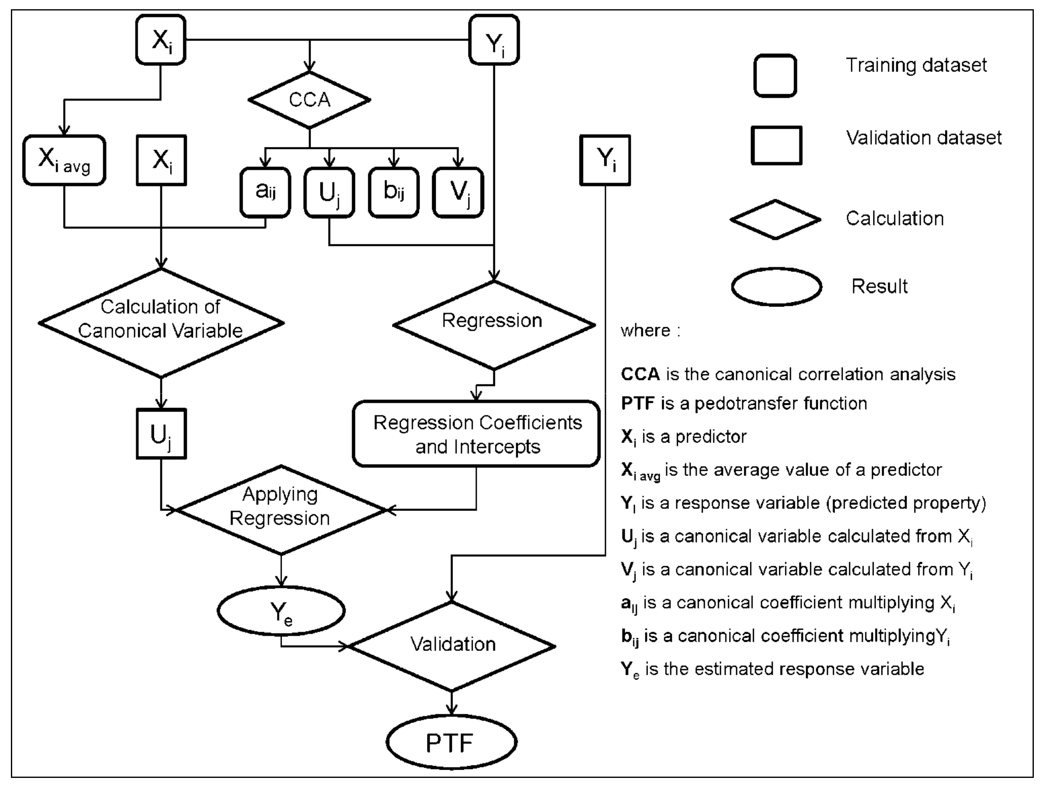
2.3.2. Canonical Correlation Analysis (CCA)

The objective of a CCA is to transform predictor (x) and response (y) variables using linear combinations in two sets of canonical variables, $U_j$ and $V_j$ respectively. The parameters are calculated such that the correlation between canonical variables $U_j$ and $V_j$ is maximal. However, the internal correlation of the different components of each canonical variable is minimal. Canonical variables are generated using canonical coefficients ($a_{ij}$ and $b_{ij}$) and mean-centered variables (see Equations (3) and (4)).

$$U_j={\displaystyle \sum }_{i,j=1}^N(x_i-\overline{x_i})a_{ij},$$

(3)

$$V_j={\displaystyle \sum }_{i,j=1}^N(y_i-\overline{y_i})b_{ij},$$

(4)

where x_i is an observed value of a predictor, $\overline{x_i}$ is the average value of the predictor, y_i is an observed value of a response variable, and $\overline{y_i}$ is the average value of the response variable.

One of the attractive features of CCA is that canonical variables enable grouping redundant properties into a single component. Each canonical variable related to predictors ($U_j$) contains the maximum amount of information available having an optimal correlation with the canonical variable related to the response variables ($V_j$) [50]. However, in the context of the PTF development, the goal is not to generate canonical response variables $V_j$, but rather to predict response variables. Nevertheless, if there are interconnections between secondary and primary soil properties, it can be useful to perform a CCA with predictor and response variables and a multiple regression using $U_j$ as predictors of the response variables. In doing so, a maximum of information derived from the predictors is translated into $U_j$ canonical variables, which are then optimized according to the $V_j$ canonical variables computed from the response variables. It has been demonstrated that performing a regression on a system of canonical variables gives satisfactory results when used in an estimation process in the presence of collinearity [51].

The CCA-PTF development method is depicted in Figure 2. The first step of this method is to conduct a CCA with predictors $x_i$ (clay, silt, OC, and CF) and response variables $y_i$ (θ₁₅₀₀, θ₃₃, ρ_b, and K_sat) according to a training dataset for a given soil horizon. The next step is to keep the $U_j$ canonical variables and their canonical coefficients $a_{ij}$. $V_j$ canonical variables and their canonical coefficients $b_{ij}$ are not used. As mentioned before, each $U_j$ has a maximum correlation with its corresponding $V_j$ calculated from the response variables, $y_i$. A multiple regression is then performed for each of the response variables and $U_j$ variables from the training dataset. Only $U_j$ variables with a significant regression coefficient are retained in the regression (the coefficient must differ from 0 with a significance p-value of 5%). Regressions are then recomputed for all other response variables from the training dataset. The next step is to produce a set of canonical variables using predictors $x_i$ from a validation dataset, as well as the previously generated mean predictors and canonical coefficients $a_{ij}$. Regression parameters and previously determined intercepts (from the training dataset) are then used with the new canonical variables to estimate the response variable $y_i$. Finally, accuracy of the results is assessed by comparing the estimated response variables and response variables from the validation dataset.

2.3.3. Accuracy Assessment

To evaluate the estimation quality of the developed PTFs, the determination coefficient (R²), root-mean-square error (RMSE), bias, and Nash–Sutcliffe efficiency (NSE) index [52] were calculated for each secondary soil property during the accuracy assessment procedure. The RMSE (Equation (5)) quantifies the contribution of systematic and random errors expressed in measurement units, and the bias (Equation (6)) quantifies the systematic error (over- or underestimation), also expressed in measurement units [53]. The NSE (Equation (7)) is used to characterize the goodness of fit of a model. NSE values can range from −∞ to 1. An NSE value equal to 1 indicates perfect modeling, while a value below 0 means that the average of measured values is a better predictor than the model predictions. When the NSE value is equal to 0, the performance of both predictors is similar. A classification of the NSE applied to the PTFs is detailed in

Table 1. Classification of the Nash–Sutcliffe efficiency (NSE) index.

NSE Value	Qualification
≤0	Unacceptable
0 to 0.4	Weak (unsatisfactory)
0.4 to 0.6	Moderate (satisfactory)
0.6 to 0.8	Good (satisfactory)
0.8 to 1	Optimal (satisfactory)

.

A cross-validation procedure was conducted on the developed PTFs. Each horizon dataset was randomly split into two datasets: one for training and one for validation [54]. A ratio of 1: 4 was used to randomly split each horizon dataset into a training dataset (75%) and a validation dataset (25%). Minimum and maximum values for each response variable were assigned to the training dataset to prevent extrapolation. This procedure was repeated 10,000 times from the original horizon dataset. At each loop, a PTF was calculated from the training dataset and then applied on the validation dataset. Each metric (R², RMSE, bias, and NSE) was calculated from the estimated and the measured soil physical property of the validation dataset. At the end of the final iteration, the average and confidence intervals of each metric were calculated (probability = 95%). The existing PTFs were also evaluated at each horizon using the corresponding dataset. The same metrics were calculated but in a context of independent validation.

$$RMSE=\sqrt{\frac{1}{N}{\displaystyle \sum }_{i=1}^N{\left(E_i-M_i\right)}^2},$$

(5)

$$Bias=\frac{1}{N}{\displaystyle \sum }_{i=1}^N\left(E_i-M_i\right),$$

(6)

$$NSE=1-\frac{{\displaystyle {\displaystyle \sum }_{i=1}^N}{\left(E_i-M_i\right)}^2}{\sum (M_i-\overline{M})},$$

(7)

where E is the estimated value, M is the measured value, and N is the number of samples.

3. Results

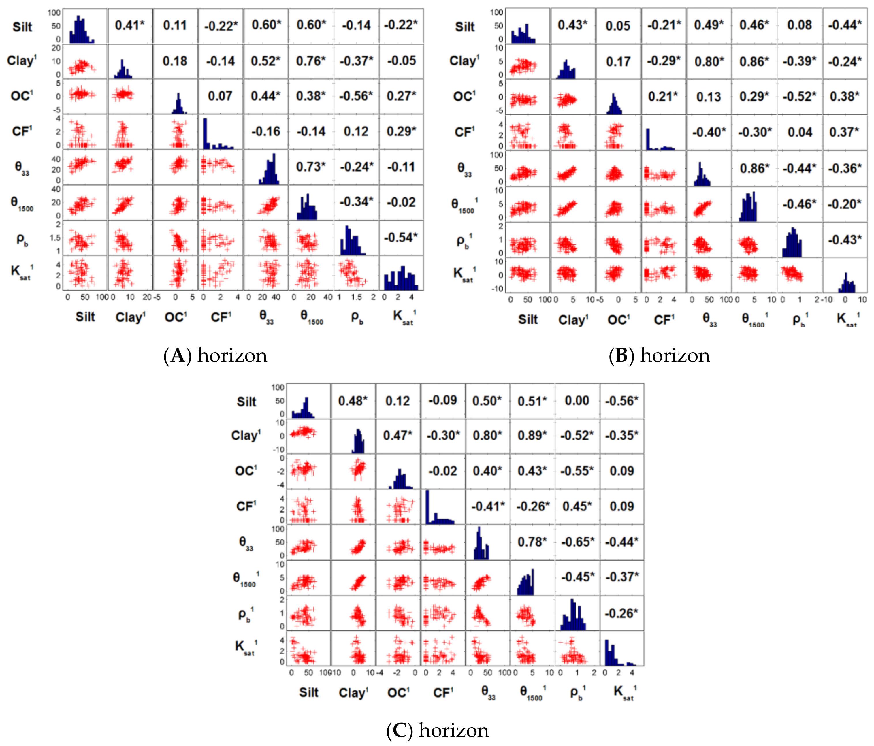
3.1. Data Exploration

Means and coefficients of variation (CV) were calculated for each soil parameter and horizon dataset (

Table 2. Statistics of soil properties; CV, coefficient of variation.

Soil Properties		A Horizon		B Horizon		C Horizon
		Mean	CV	Mean	CV	Mean	CV
Primary	Silt (%)	35.14	0.42	33.86	0.52	35.10	0.45
	Clay (%)	21.82	0.62	22.23	0.89	18.89	0.94
	OC (%)	2.21	0.49	0.46	1.02	0.16	0.81
	CF (%)	3.62	1.81	7.85	1.63	7.79	1.63
Secondary	θ33 (%)	31.66	0.20	28.36	0.37	29.25	0.41
	θ1500 (%)	15.48	0.38	14.18	0.62	13.30	0.69
	ρb (g·cm−3)	1.33	0.12	1.50	0.14	1.60	0.15
	Ksat (cm·h−1)	22.30	1.23	14.95	1.59	5.56	2.51
	Sample size	88		121		95

). The mean percentage of OC, θ₁₅₀₀, and K_sat decreased with soil depth (from the A to the C horizon), while ρ_b increased from the A to the C horizon. OC is the result of plant decomposition and manure application, which take place within the top 20 cm soil layer. Soil compaction increases with depth ρ_b and reduces the porosity, thus determining the available space for water. It should be noted that CVs were generally lower than 1, except for CF and K_sat, which often show very high spatial variability at the field scale [55].

Statistical analysis of soil parameters was conducted on normally distributed data. The data transformations applied to each variable (when required) are shown in

Table 3. Normal distribution transformations of soil properties.

Soil Properties		A Horizon	B Horizon	C Horizon
Primary	Silt	–	–	–
	Clay	Box–Cox, λ = 0.4072	Box–Cox, λ = 0.1248	Box–Cox, λ = 0.1659
	OC	Box–Cox, λ = 0.2750	Box–Cox, λ = −0.0874	Box–Cox, λ = 0.1664
	CF	ln(x + 1)	ln(x + 1)	ln(x + 1)
Secondary	θ33	–	–	–
	θ1500	–	Box–Cox, λ = 0.2258	Box–Cox, λ = 0.2206
	ρb	–	Box–Cox, λ = 2.4488	Box–Cox, λ = 2.2516
	Ksat	ln(x + 1)	ln(x + 1)	ln(x + 1)

. Distributions, scatter plots, and Pearson’s correlation coefficients of both primary and secondary soil properties are illustrated in a matrix form for each soil horizon in Figure 3. The cross-correlation coefficients obtained between predictors were below 0.5, absolute value, at all soil horizons. However, these correlation coefficients were often significant, which means that certain predictors were collinear (i.e., silt, clay, etc.).

Most of the highest correlation coefficients, in absolute values, were obtained between predictors and response variables. θ₃₃ was positively correlated with silt (0.60, 0.49, and 0.50) and clay (0.52, 0.80, and 0.80), at the A, B, and C horizons, respectively. θ₁₅₀₀ was also positively correlated with silt (0.60, 0.46, and 0.51) and clay (0.76, 0.86, and 0.89), at the A, B, and C horizons, respectively. Clay content has an impact on water retention properties, as water content tends to be greater in soils that have a high clay percentage. A negative correlation was observed between ρ_b and OC percentage (−0.56, −0.52, and −0.55) at the A, B, and C horizons, respectively. In the C horizon, clay percentage was negatively correlated to ρ_b (−0.52). K_sat had weak correlation coefficients with all predictors for the A horizon. However, negative correlations of −0.44 and −0.56 with silt percentage were observed at the B and C horizons, respectively. The effect of CF on K_sat can be either negative or positive, depending on CF location. When CFs are on the soil surface, they increase infiltration by preventing the soil from sealing, but they reduce infiltration when contained within the soil layer [56,57,58]. The relationship between OC and K_sat can also vary. Some authors argue that OC increases K_sat by improving soil structure [59], while others conclude that it decreases K_sat because OC retains water, its aggregates increase tortuosity, and the quality/kind of organic matter may affect hydraulic properties [23].

3.2. Stepwise Forward Regression-Based Pedotransfer Functions

Table 4. Standardized (St. *) and non-standardized (Non st. **) regression coefficients obtained by stepwise forward regression.

Response Variables	θ33 (%)		θ1500 (%)		ρb (g cm−3)		Ksat (cm h−1)
Horizon	Coefficients		Coefficients		Coefficients		Coefficients
	St. *	Non st. **	St. *	Non st. **	St. *	Non st. **	St.*	Non st. **
A
Intercept	–	18.3997	–	–	–	1.5525	–	1.7828
Silt	2.7664	0.1903	1.8400	0.1397	–	–	–	–
Clay 1	1.3949	0.6302	3.1261	1.5100	−0.0431	−0.0195	–	–
OC 1	3.1786	4.1219	1.6514	2.2206	−0.1250	−0.1623	0.3497	0.4543
CF 1	–	–	–	–	–	–	0.4054	0.3674
R2	0.59		0.69		0.50		0.2694
RMSE	4.34		3.3012		0.14		42.87
B
Intercept	–	10.6471	–	0.7646	–	0.6123	–	3.4065
Silt	1.6178	0.0943	0.1440	0.0084	0.1157	0.0067	−0.58	−0.0340
Clay 1	7.2655	5.4649	0.9087	0.6835	−0.1494	−0.1123	–	–
OC 1	1.2338	1.1441		–	−0.2076	−0.1925	0.6102	0.5658
CF 1	−2.3443	−1.6381		–	–	–	0.3696	0.2583
R2	0.70		0.73		0.49		0.28
RMSE	6.03		4.73		0.18		29.035
C
Intercept	–	21.2177	–	0.6406	–	−0.0217	–	3.7264
Silt	2.8625	0.1815	0.1788	0.0113	0.1198	0.0076	−0.5898	−0.0374
Clay 1	6.3755	4.0055	1.0586	0.6651	−0.1188	−0.0747	−0.2486	−0.1562
OC 1	2.3907	4.1961	–	–	−0.2278	−0.3998	0.2729	0.4790
CF 1	−3.5305	−2.6145	–	–	0.1444	0.1069	–	–
R2	0.68		0.74		0.52		0.23
RMSE	7.39		4.78		0.21		25.92

shows the regression coefficients obtained using the SFR method. Standardized coefficients show the weight accorded to predictors in the developed PTF (coefficients without unit effect measurement).

For the estimation of θ₃₃, the A horizon PTF used the following predictors: OC, silt, and clay percentages, listed by decreasing weight. The PTFs developed for the B and C horizons had the highest weight of clay, followed by CF percentage, and small weights of silt and OC. The standardized regression coefficients of OC were stronger for the A horizon, which is explained by the abundance of OC on the soil surface.

In the case of the estimation of θ₁₅₀₀, clay and silt, followed by OC, were retained as predictors for the A horizon. Coefficient values were positive, indicating that increases in these properties correspond to increases in θ₁₅₀₀. At the B and C horizons, clay percentage coefficients were broadly higher, followed by silt percentage. As shown in Figure 3, the correlation between θ₁₅₀₀ and clay was the highest at each soil horizon. Increasing clay content increases the soil water-holding capacity.

In the case of the estimation of ρ_b, a negative weight was given to OC and clay content for all horizons. As mentioned above, a negative correlation was observed between ρ_b and these predictors. At the B horizon a moderate positive weight was also given to silt content. At the C horizon, moderate positive weights were given to CF and silt percentages.

The predictors selected for the estimation of K_sat were different for each horizon (Table 4). At the A horizon, only CF and OC were selected with a positive weight. OC was also given a positive weight at the B horizon, followed by silt with a negative weight, and CF with a positive weight. At the C horizon, silt was selected with a negative weight, followed by CF (positive weight) and OC (negative weight).

3.3. Canonical Correlation Analysis-Based Pedotransfer Functions

Correlations between canonical variables U and V are presented in

Table 5. Correlation coefficients between canonical variables U and V calculated for each soil horizon.

	A Horizon	B Horizon	C Horizon
U1,V1	0.89	0.89	0.90
U2,V2	0.52	0.69	0.66
U3,V3	0.43	0.28	0.40
U4,V4	0.26	0.07	0.01

. As expected, the correlation decreased from the first to the fourth canonical variable. The weights accorded by the PTF to a predictor were determined using a combination of the weight of the predictors related to the canonical variables (

Table 6. Canonical coefficients a_ij and correlation coefficients generated for each canonical variable.

Property	U1		U2		U3		U4
	aij	R	aij	R	aij	R	aij	R
Horizon A
Silt	0.0217	0.61	0.0118	0.29	0.0382	0.52	−0.0620	−0.52
Clay 1	0.2133	0.74	0.3311	0.59	−0.1730	−0.10	0.2647	0.31
OC 1	0.7723	0.74	−1.0277	−0.60	−0.3633	−0.29	−0.0224	−0.04
CF 1	−0.0673	−0.20	0.2768	0.14	−0.6684	−0.80	−0.5843	−0.54
θ33	–	0.75	–	−0.06	–	0.10	–	−0.12
θ1500 1	–	0.79	–	0.23	–	0.03	–	−0.01
ρb 1	–	−0.63	–	0.27	–	0.14	–	−0.09
Ksat 1	–	0.13	–	−0.07	–	−0.42	–	0.00
Horizon B
Silt	−0.0101	−0.58	−0.0329	−0.45	−0.0066	−0.07	−0.0551	−0.68
Clay 1	−0.6223	−0.97	0.1766	0.10	−0.4248	−0.16	0.4601	0.14
OC 1	−0.0625	−0.24	0.7298	0.83	0.4645	0.18	−0.4714	−0.47
CF 1	0.1170	0.47	0.1326	0.38	−0.7419	−0.77	−0.1152	−0.22
θ33	–	−0.84	–	−0.01	–	0.07	–	−0.02
θ1500 1	–	−0.81	–	0.03	–	−0.09	–	0.0185
ρb 1	–	0.32	–	−0.59	–	−0.10	–	−0.01
Ksat 1	–	0.30	–	0.60	–	−0.05	–	−0.02
Horizon C
Silt	0.0103	0.58	0.0458	0.65	−0.0372	−0.31	−0.0428	−0.37
Clay 1	0.4811	0.97	0.0788	0.04	0.5646	0.20	0.4199	0.10
OC 1	0.3016	0.54	−1.3032	−0.62	−0.4637	0.05	−1.4239	−0.57
CF 1	−0.1148	−0.43	0.2432	0.20	0.6708	0.72	−0.3155	−0.51
θ33	–	0.81	–	0.00	–	−0.15	–	0.00
θ1500 1	–	0.88	–	0.07	–	0.08	–	0.00
ρb 1	–	−0.50	–	0.53	–	0.07	–	0.00
Ksat 1	–	−0.39	–	−0.46	–	0.19	–	0.00

) and the weight given to the canonical variables obtained by regression (

Table 7. Regression coefficients between canonical variables and response variables; p ≤ 0.05.

Response Variables
Horizon A	θ33	θ1500 1	ρb 1	Ksat 1
Intercept	32.4341	15.7784	1.2982	2.4895
U1	5.1244	4.6768	−0.1266	–
U2	–	1.3632	0.0546	–
U3	–	–	–	−0.5768
U4	–	–	–	–
R2	0.57	0.69	0.48	0.19
RMSE	4.47	3.28	0.14	43.40
Horizon B	θ33	θ1500 1	ρb 1	Ksat 1
Intercept	28.7736	3.3318	0.7082	1.8381
U1	−9.4011	−0.9740	0.1305	0.4429
U2	–	–	−0.2357	0.8850
U3	–	–	–	–
U4	–	–	–	–
R2	0.70	0.71	0.47	0.23
RMSE	6.08	4.93	0.18	29.55
Horizon C	θ33	θ1500 1	ρb 1	Ksat 1
Intercept	29.5832	3.1433	0.8339	1.1059
U1	10.6868	1.1536	−0.2313	−0.4499
U2	–	–	0.2428	−0.5372
U3	–	–	–	0.2169
U4	–	–	–	–
R2	0.66	0.73	0.50	0.27
RMSE	7.66	4.89	0.21	25.41

) between response variables. Because of the scale effect, it is recommended to use correlation coefficients to describe the contribution of a predictor to a canonical variable, instead of interpreting canonical coefficients a_ij [60]. Canonical coefficients are only used to calculate canonical variables.

3.3.1. Contribution of Predictors to Canonical Variables

At the A horizon, the predictors making the highest contribution to U₁ were OC and clay percentages, followed by silt with a moderate correlation coefficient (Table 6). The main contributions to U₁ at the B and C horizons came from the clay percentage followed by the silt percentage and OC. The OC contribution to the B and C horizons was weak compared to its contribution to the A horizon. The dominant contributions to U₂ at the A horizon (highest negative correlation) came from OC and clay content, with a similar contribution but with positive value (Table 6). OC was also the predictor with the highest correlation at the B horizon, but with a slightly lower and positive value. Silt percentage made a moderate negative contribution. At the C horizon, the contributor with the highest correlation was silt, followed by OC, with a similar absolute contribution. Thus, U₂ is essentially explained by the OC contribution, although, depending on the horizon, clay and silt contribute to that canonical variable. For all soil horizons, the predictor with the highest correlation with U₃ was CF (Table 6). It should be noted that a negative correlation was observed with both the A and B horizons. It was not possible, regarding U₄, to identify one or two predictors that were applicable to all three horizons. In terms of predictive power, the first canonical variable U₁, showed the highest correlation with most response variables, in all horizons. The strength of correlation then decreased from U₂ to U₄ with most response variables.

3.3.2. Regressions Using Canonical Variables as Predictors

For the estimation of θ₃₃, U₁ was the only canonical variable selected for all horizons, with correlation coefficients varying between 0.75 and 0.84 (Table 6). U₁ was essentially defined by clay and silt percentages in these horizons, but OC also made a strong contribution in the A horizon. The weights given to the predictors were similar to those obtained with the SFR approach. The results of the regression used to estimate θ₁₅₀₀ were similar to those estimating θ₃₃, in terms of predictor weight (Table 6) and regression coefficients of the canonical variables (Table 7). A strong correlation between θ₁₅₀₀ and θ₃₃ was previously observed (Figure 3). U₁ was strongly correlated with θ₁₅₀₀ (Table 6), which explains why it was once again retained in the regression (Table 7). Clay also had a large impact on these functions. U₂ was selected for the A horizon, which was mostly correlated with clay and OC contents. Again, the resulting PTF was similar to the one developed with the SFR approach.

For each horizon, U₁ and U₂ were selected to estimate ρ_b (Table 7). As previously mentioned, U₁ was explained by clay, silt, and OC percentages, while U₂ was mostly explained by OC, followed by silt percentage for B and C horizons. OC was more important in the A horizon and decreased with increasing soil depth. Multiplication of the correlation coefficient (Table 6) by the regression coefficients (Table 7) gives the effect of a predictor on a response variable. Negative weights were given to clay and OC percentages. Silt had a negative effect at the A horizon and a positive effect at the B and C horizons. Organic matter has a lower ρ_b than mineral material; thus, the overall ρ_b is reduced when the organic matter percentage in mineral soil increases. This could explain the negative effect of OC in both CCA- and SFR-derived PTFs for ρ_b prediction. The negative contribution of clay in PTFs predicting ρ_b was also observed by Jones [61].

In the case of K_sat estimation, the correlation with canonical variables was different for each horizon. For the A horizon, K_sat was slightly correlated to U₃ (negatively; Table 6). The regression between K_sat and its canonical variables gave a negative weight to U₃ (Table 7). CF was the main predictor for U₃ (negative weight), followed by silt (positive weight) and OC (negative weight). The resulting combination of correlation and weight showed the positive effects of OC and CF, and the negative effect of silt on K_sat. These results are consistent with the previously conducted cross-correlation analysis (Figure 3). For the B horizon, the regression selected U₂ and U₁ with positive weights (Table 7). U₂ was correlated with K_sat, followed by U₁ (moderately). As a result, OC was the most contributing predictor (positive effect), followed by silt and clay (negative), and CF (small positive). These results are consistent with those of the cross-correlation analysis (Figure 3), where K_sat was positively correlated with OC and CF, and negatively correlated with silt and clay percentages. For the C horizon, U₃ was selected as a predictor with positive weight, while U₂ and U₁ were selected with negative weights. The correlation between U₁ and K_sat was similar to that obtained with U₂ in absolute terms. However, the correlation obtained with U₃ was weak (Table 6). The negative coefficients for U₁ and U₂ indicate that clay and silt made a negative contribution to this PTF, while the effect was negative for OC. The positive correlation coefficient for U₃ was explained by a positive effect of CF.

Neither the SFR nor the CCA method selected identical predictors at each horizon. However, it is well known that higher clay-to-silt percentages increase soil water retention and that higher CF reduces this property [62]. In this study, increased OC content led to increased K_sat. However, it has been demonstrated that the effect of clay is positive when its proportion is less than 30%, but varied and more complex when the proportion is higher [63].

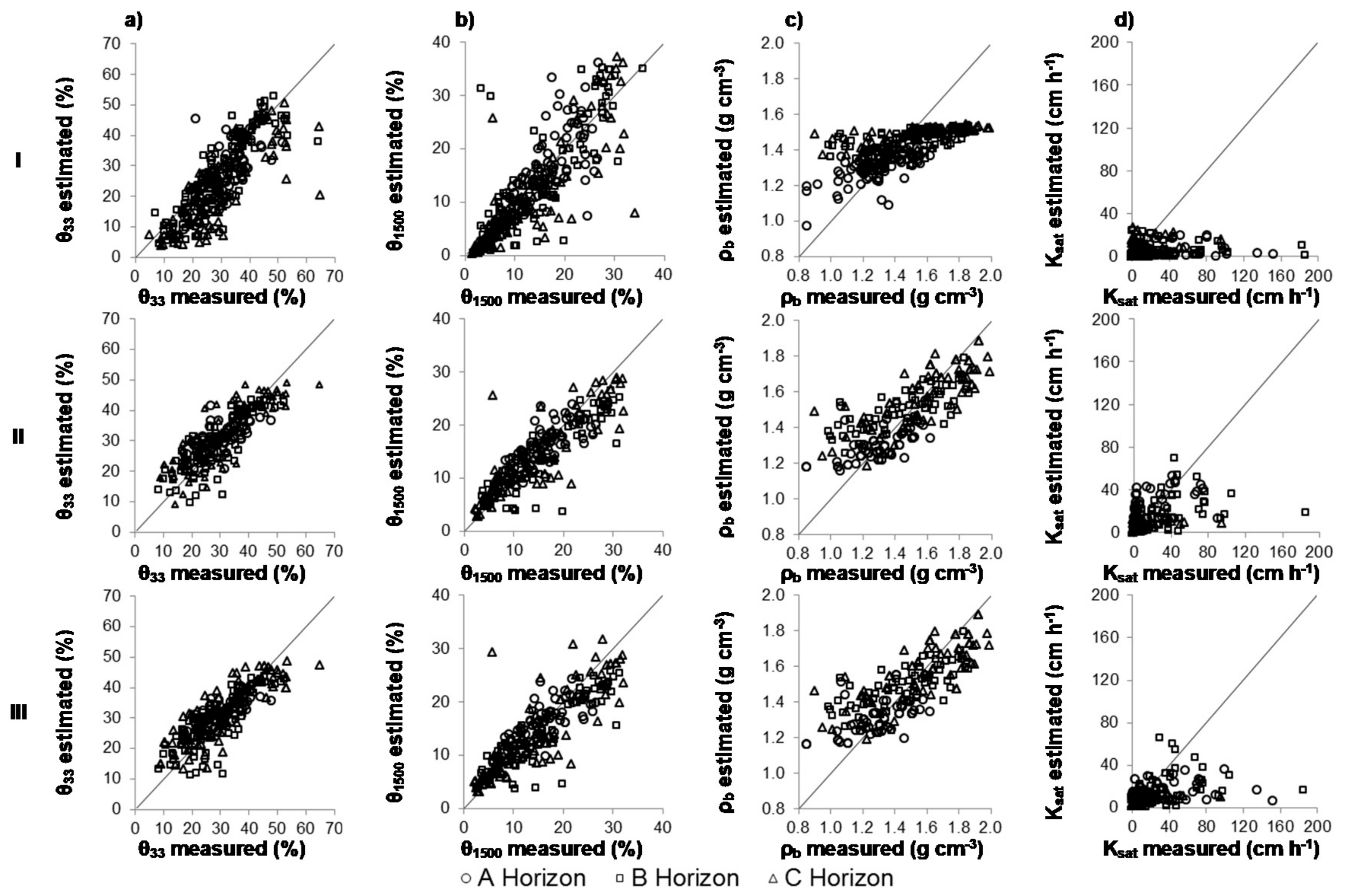
3.4. Validation and Comparison with the Saxton and Rawls’s PTFs

Table 8. Accuracy evaluation of existing and developed PTFs. Values in bold are the best performances. The values in square brackets are the maximum and minimum values calculated from the simulations.

Property/Horizon	Saxton & Rawls * PTFs				Stepwise Forward Regression				Regression with CCA
	R2	NSE	RMSE	Bias	R2	NSE	RMSE	Bias	R2	NSE	RMSE	Bias
θ33 (%)
A	0.45	−0.26	7.6	−3.4	0.54 [0.540, 0.544]	0.47 [0.466, 0.470]	4.3 [4.29, 4.31]	0.4 [0.41, 0.45]	0.53 [0.525, 0.529]	0.47 [0.467, 0.471]	4.4 [4.36, 4.38]	0.4 [0.34, 0.38]
B	0.74	0.54	7.5	−3.5	0.68 [0.675, 0.678]	0.63 [0.626, 0.629]	5.9 [5.91, 5.93]	0.8 [0.79, 0.83]	0.68 [0.679, 0.682]	0.63 [0.630, 0.633]	5.9 [5.86, 5.88]	0.8 [0.78, 0.82]
C	0.66	0.34	10.7	−7.2	0.69 [0.691, 0.693]	0.65 [0.652, 0.655]	7.4 [7.34, 7.37]	0.5 [0.42, 0.48]	0.70 [0.697, 0.699]	0.66 [0.660, 0.663]	7.3 [7.28, 7.31]	0.5 [0.51, 0.56]
θ1500 (%)
A	0.56	0.32	4.8	−0.2	0.68 [0.677, 0.680]	0.67 [0.671, 0.675]	3.2 [3.19, 3.21]	0.2 [0.24, 0.26]	0.66 [0.659, 0.662]	0.61 [0.609, 0.613]	3.3 [3.32, 3.34]	0.3 [0.25, 0.28]
B	0.72	0.55	6.0	−0.2	0.81 [0.810, 0.812]	0.76 [0.755, 0.757]	4.1 [4.05, 4.07]	−1.3 [−1.31, −1.28]	0.81 [0.810, 0.812]	0.75 [0.744, 0.747]	4.1 [4.05, 4.07]	−1.3 [−1.31, −1.28]
C	0.71	0.58	6.0	−2.2	0.79 [0.793, 0.797]	0.77 [0.763, 0.767]	4.4 [4.35, 4.38]	−0.4 [−0.44, −0.41]	0.74 [0.740, 0.744]	0.70 [0.693, 0.698]	5.0 [4.94, 4.97]	−0.5 [−0.52, −0.48]
ρb (g·cm−3)
A	0.48	0.46	0.15	0.00	0.28 [0.276, 0.281]	0.16 [0.151, 0.160]	0.15 [0.146, 0.147]	0.00 [0.002, 0.003]	0.27 [0.268, 0.273]	0.13 [0.128, 0.136]	0.15 [0.147, 0.148]	0.01 [0.014, 0.015]
B	0.47	0.29	0.21	−0.04	0.33 [0.333,0.336]	0.27 [0.272, 0.276]	0.18 [0.181, 0.181]	0.01 [0.004, 0.005]	0.32 [0.315, 0.319]	0.26 [0.256, 0.260]	0.18 [0.183, 0.184]	0.01 [0.005, 0.006]
C	0.40	0.12	0.28	−0.08	0.53 [0.525, 0.529]	0.48 [0.476, 0.480]	0.18 [0.179, 0.179]	0.00 [−0.001, 0.000]	0.52 [0.517, 0.521]	0.47 [0.470, 0.474]	0.18 [0.180, 0.181]	0.00 [−0.001, 0.000]
Ksat (cm·h−1)
A	0.00	−0.28	50.0	−23.5	0.15 [0.146, 0.150]	−0.10 [−0.100, −0.099]	30.7 [30.6, 30.8]	−12.5 [−12.6, −12.4]	0.13 [0.129, 0.133]	−0.10 [−0.107, −0.101]	31.2 [31.0, 31.3]	−12.7 [−12.8, −12.6]
B	0.05	−0.14	34.3	−13.8	0.42 [0.418, 0.423]	0.29 [0.287, 0.292]	22.9 [22.8, 23.1]	−6.7 [−6.8,−6.6]	0.37 [0.365, 0.370]	0.23 [0.232, 0.238]	23.5 [23.4, 23.6]	−6.7 [−6.8, −6.6]
C	0.11	−15.51	25.5	−3.3	0.38 [0.381, 0.386]	−0.08 [−0.113, −0.046]	12.3 [12.2, 12.4]	−2.6 [−2.7, −2.6]	0.38 [0.377, 0.383]	−0.15 [−0.185,−0.106]	12.5 [12.4, 12.6]	−2.6 [−2.7, −2.6]

presents accuracy assessment results of the PTFs (R², RMSE, NSE index, and bias) for both developed methods (SFR and CCA) and for Saxton and Rawls’s PTFs (2006), which are further referred to as PTFs’S&R.2006.

Accuracy assessment plots of the PTFs developed to estimate θ₃₃ are presented in Figure 4a. PTFs’S&R.2006 for A and C horizons had a lower R² than both the SFR- and the CCA-derived PTFs. However, they also had the best R² for the B horizon. Nevertheless, PTFs’S&R.2006 were more erroneous in terms of RMSE and bias. Estimation quality for θ₃₃ was very similar with both the SFR and the CCA methods (R² values ranging from 0.53 to 0.70). In terms of NSE, the performance of PTFs’S&R.2006 was unsatisfactory with a negative value for the A horizon, satisfactory for the B horizon (moderately), and unsatisfactory for the C horizon (weak). The SFR- and the CCA-derived PTFs performed equally well with a moderate NSE for the A horizon and a good NSE for the B and C horizons.

Accuracy assessment plots of the PTFs developed to estimate θ₁₅₀₀ are illustrated in Figure 4b. The same pattern as that observed with PTFs’S&R.2006 used to predict θ₃₃ was found with θ₁₅₀₀. In comparison with θ₃₃, the performance of θ₁₅₀₀ PTFs was slightly higher. The R² values were good, especially for the B and C horizons. In terms of NSE, the performance of PTFs’S&R.2006 was unsatisfactory for the A horizon (weak) and satisfactory for the B and C horizons (moderate). The SFR-derived PTFs outperformed the CCA-derived PTFs; however, for both methods, the NSE was qualified as good for all horizons.

Accuracy assessment plots of the PTFs developed to estimate ρ_b are illustrated in Figure 4c. PTFs’S&R.2006 gave the best ρ_b prediction for the A horizon, with the highest R² and lowest RMSE (0.48 and 0.15 g·cm⁻³). For this horizon, the SFR- and CCA-derived PTFs led to the same R² and RMSE values (0.28 and 0.15 g·cm⁻³, respectively). Both methods also generated the same R² and RMSE values at the B and C horizons. In terms of NSE, the performance of PTFs’S&R.2006 was satisfactory (moderate) for the A horizon and unsatisfactory (weak) for the B and C horizons. The SFR- and the CCA-derived PTFs performed equally well with a weak NSE for the A and B horizons and a moderate NSE for the C horizon.

Accuracy assessment plots of the PTFs generated to estimate K_sat are illustrated in Figure 4d. At the A horizon, the SFR method performed better than the CCA method. In comparison to PTFs’S&R.2006 and the CCA-derived PTF, the SFR-derived PTF had a higher R² and a lower RMSE. However, its estimation quality remained weak (R² of 0.15 and RMSE of 30.7 cm·h⁻¹). The estimation quality of PTFs’S&R.2006 was poor for the B horizon. For this horizon, both CCA- and SFR-derived PTFs were slightly more accurate (R² of 0.42 and RMSE of 22.9 cm·h⁻¹ for SFR-PTFs). At the C horizon, results were similar to those of the B horizon, but with lower RMSE (12.3 cm·h⁻¹). In terms of NSE, PTFs’S&R.2006 were unsatisfactory for all horizons (negative values). The same conclusion was noted for both SFR- and CCA-derived PTFs, but with weak positive values for the B horizon. The performance remained unsatisfactory. The SFR-derived PTFs slightly outperformed the CCA-derived PTFs; however, for both methods, the NSE was qualified as unacceptable for the A and C horizons and weak for the B horizon.

4. Discussion

The above results demonstrate the potential of the primary soil properties (clay, silt, OC, and CF percentages) to estimate the secondary soil properties (θ₁₅₀₀, θ₃₃, ρ_b, and K_sat) for different horizons (A, B, and C) with varying accuracy rates. The hypothesis tested in this study was the ability of locally trained PTFs, using SFR and CCA algorithms, to produce more accurate estimates than the PTFs’S&R.2006 that were trained with global soil data. As expected, our results highlighted that, in most cases, locally trained PTFs achieved the best accuracy in estimating secondary soil properties.

In the case of θ₃₃, PTFs’S&R.2006 results were systematically underestimated. This underestimation increased in the deeper horizons (soil depth), which is unsurprising, since the PTFs’S&R.2006 were developed using A horizon soil samples. Both the SFR- and CCA-derived PTFs had moderate performances for the A horizon and good performances for the B and C horizons. Pollacco [64] evaluated the performance of eight different PTFs to predict θ₃₃. The RMSE values for these PTFs ranged from 5.7% to 11.1%, whereas they ranged from 4.3% to 7.4% for the PTFs developed in the present study, which is considered acceptable. These results are comparable to the θ₃₃ accuracy assessment results found in the literature [2,28,65].

In the case of θ₁₅₀₀, the PTFs’S&R.2006 were again less accurate with a lower R² and higher RMSE and bias than the SFR- and CCA-derived PTFs for the A horizon. Methods developed using SFR and CCA showed similar performance. The SFR method produced slightly higher R² and lower RMSE and bias at the A and C horizons. The performance of the two methods was identical at the B horizon. In fact, the clay percentage was strongly correlated with θ₁₅₀₀ (Figure 3). The reason is that the SFR method selected clay as a predictor, while the CCA method selected the canonical variable to which clay was the major contributor. Both SFR- and CCA-derived PTFs were satisfactory (good) for all horizons. Again, RMSE values obtained in this study (ranging from 3.2% to 5.0%) outperformed the RMSE values obtained by Pollacco [64] (ranging from 4.7% to 7.5%). These results are acceptable and similar to the θ₁₅₀₀ results found in the literature [2,28,65].

In the case of ρ_b estimation, PTFs’S&R.2006 were well adapted to the A horizon. This is likely because the PTFs’S&R.2006 use volumetric water content at saturation (obtained by a PTF) to generate normal density, which is then used with CF to predict ρ_b, and they were originally calibrated using the A horizon data. At the B horizon, in terms of estimation errors, our PTFs were less erroneous than the PTFs’S&R.2006. The latter produced the highest R² (0.47) at the B horizon, but it also showed an important RMSE value (0.21 g·cm⁻³). Both the SFR- and CCA-derived PTFs outperformed PTFs’S&R.2006 at the C horizon in terms of R² and RMSE (0.53 vs. 0.40 and 0.18 vs. 0.28 g·cm⁻³). A comparison with PTFs available in the literature [2,66,67] suggests that RMSE should range between 0.13 and 0.23 g·cm⁻³, which was the case.

In the case of K_sat, the estimation quality was poor for all horizons. The SFR method slightly outperformed the CAA method at the B horizon, and both methods performed poorly for the A and C horizons yet showed higher accuracy than PTFs’S&R.2006 estimates. In fact, the soil of the A horizon is frequently disturbed by tillage, plant root penetration, and field alterations that modify soil structure. This variation in soil structure could explain the high variability observed in saturated soil hydraulic conductivity (Table 2), which is not explained by soil texture and OC alone. In addition, K_sat and CF showed great variability; consequently, averages were less representative for these properties than for other soil properties. Jorda et al. [26] found that the most influential predictor for K_sat was land use. They noted a difference between samples in conventional agricultural sites and non-tilled sites. These results demonstrate the importance of soil structure to K_sat estimations. The lack of selected predictors that relate to soil structure might explain the difficulty to estimate K_sat. Prediction of this physical property could, however, be improved by adding morphological predictors such as soil structure and drainage information.

Overall, the SFR-derived PTFs were equal to or more accurate than the CCA-derived PTFs and were more accurate than the PTFs’S&R.2006. In fact, the major difference between CCA and SFR methods is that CCA always uses all available predictors to develop its canonical variables, whereas the SFR method uses a selection strategy to determine explanatory predictors. The use of all predictors may introduce noise, which explains the observed difference in performance between the two developed PTFs. Even in the few cases where the CCA-derived PTFs outperformed the SFR-derived PTFs (θ₃₃ for horizon C, for example (Table 8)), we still recommend using the SFR-derived PTF because of the small significant difference in results and its easier execution.

5. Conclusions

In this study, four secondary soil properties—bulk density (ρ_b), saturated hydraulic conductivity (K_sat), and volumetric water content (θ) measured at two matric potentials, −33 kPa (field capacity (θ₃₃)) and −1500 kPa (permanent wilting point (θ₁₅₀₀))—were estimated for A, B, and C horizons for agricultural areas of southern Quebec, Canada. Estimates were performed using existing functions from Saxton and Rawls’s PTFs (2006) and new PTFs trained using the stepwise forward regression (SFR) and canonical correlation analysis (CCA) algorithms. Primary soil properties (clay, silt, organic carbon, and coarse fragment percentages) were used as inputs for estimating the secondary soil properties. All PTFs (equations are available in Appendix A) were assessed using the cross-validation technique from which the R², Nash–Sutcliffe efficiency (NSE), root-mean-square error (RMSE), and bias were generated. Except for ρ_b for A and B horizons that showed higher accuracy in terms of NSE and R² and equal accuracy in terms of RMSE and bias, all the other physical secondary soil properties estimated using either SFR- or CCA-derived PTFs were more accurate, particularly for θ₃₃ and θ₁₅₀₀. According to the NSE index, θ₁₅₀₀ showed the best performance (qualified as good), followed by θ₃₃ (qualified as moderate to good) for the different horizons. The NSE index for ρ_b was qualified as low, while the NSE index for K_sat was qualified as unacceptable to low for the best performances for the different horizons. It is, thus, recommended to retrain the last two soil properties using other morphological predictors such as soil structure and drainage information before considering their use. Overall, the SFR method showed equal to or better performance than the CCA method.

References

1. Dobarco, M.R.; Cousin, I.; Le Bas, C.; Martin, M.P. Pedotransfer functions for predicting available water capacity in French soils, their applicability domain and associated uncertainty. Geoderma 2019, 336, 81–95. [Google Scholar] [CrossRef]
2. Kätterer, T.; Andrén, O.; Jansson, P.E. Pedotransfer functions for estimating plant available water and bulk density in Swedish agricultural soils. Acta Agric. Scand. Sect. B Soil Plant Sci. 2006, 56, 263–276. [Google Scholar] [CrossRef]
3. Morais, A.; Fortin, V.; Anctil, F. Modelling of Seasonal Evapotranspiration from an Agricultural Field Using the Canadian Land Surface Scheme (CLASS) with a Pedotransfer Rule and Multicriteria Optimization. Atmosphere-Ocean 2015, 53, 161–175. [Google Scholar] [CrossRef]
4. Castellini, M.; Iovino, M. Pedotransfer functions for estimating soil water retention curve of Sicilian soils. Arch. Agron. Soil Sci. 2019, 65, 1401–1416. [Google Scholar] [CrossRef]
5. Dashtaki, S.G.; Homaee, M.; Khodaverdiloo, H. Derivation and validation of pedotransfer functions for estimating soil water retention curve using a variety of soil data. Soil Use Manag. 2010, 26, 68–74. [Google Scholar] [CrossRef]
6. Palta, M.M.; Ehrenfeld, J.G.; Giménez, D.; Groffman, P.M.; Subroy, V. Soil texture and water retention as spatial predictors of denitrification in urban wetlands. Soil Biol. Biochem. 2016, 101, 237–250. [Google Scholar] [CrossRef]
7. Cosby, B.; Hornberger, G.; Clapp, R.; Ginn, T. A statistical exploration of the relationships of soil moisture characteristics to the physical properties of soils. Water Resour. Res. 1984, 20, 682–690. [Google Scholar] [CrossRef] [Green Version]
8. Moncada, M.P.; Penning, L.H.; Timm, L.C.; Gabriels, D.; Cornelis, W.M. Visual examinations and soil physical and hydraulic properties for assessing soil structural quality of soils with contrasting textures and land uses. Soil Tillage Res. 2014, 140, 20–28. [Google Scholar] [CrossRef] [Green Version]
9. Asgari, N.; Ayoubi, S.; Demattê, J.A.; Jafari, A.; Safanelli, J.L.; Da Silveira, A.F.D. Digital mapping of soil drainage using remote sensing, DEM and soil color in a semiarid region of Central Iran. Geoderma Reg. 2020, 22, e00302. [Google Scholar] [CrossRef]
10. Patil, N.G.; Singh, S.K. Pedotransfer Functions for Estimating Soil Hydraulic Properties: A Review. Pedosphere 2016, 26, 417–430. [Google Scholar] [CrossRef]
11. Arya, L.M.; Leij, F.J.; van Genuchten, M.T.; Shouse, P.J. Scaling parameter to predict the soil water characteristic from particle-size distribution data. Soil Sci. Soc. Am. J. 1999, 63, 510–519. [Google Scholar] [CrossRef] [Green Version]
12. Asadi, H.; Bagheri, F. Comparison of regression pedotransfer functions and artificial neural networks for soil aggregate stability simulation. World Appl. Sci. J. 2010, 8, 1065–1072. [Google Scholar]
13. Sarmadian, F.; Keshavarzi, A. Developing pedotransfer functions for estimating some soil properties using artificial neural network and multivariate regression approaches. Int. J. Environ. Earth Sci 2010, 1, 31–37. [Google Scholar]
14. Vereecken, H.; Herbst, M. Statistical regression. Dev. Soil Sci. 2004, 30, 3–19. [Google Scholar]
15. Gunarathna, M.; Sakai, K.; Nakandakari, T.; Momii, K.; Kumari, M.; Amarasekara, M. Pedotransfer functions to estimate hydraulic properties of tropical Sri Lankan soils. Soil Tillage Res. 2019, 190, 109–119. [Google Scholar] [CrossRef]
16. Nguyen, P.M.; Haghverdi, A.; De Pue, J.; Botula, Y.-D.; Le, K.V.; Waegeman, W.; Cornelis, W.M. Comparison of statistical regression and data-mining techniques in estimating soil water retention of tropical delta soils. Biosyst. Eng. 2017, 153, 12–27. [Google Scholar] [CrossRef]
17. Pachepsky, Y.; Schaap, M. Data mining and exploration techniques. Dev. Soil Sci. 2004, 30, 21–32. [Google Scholar]
18. Pachepsky, Y.; Van Genuchten, M.T. Pedotransfer functions. In Encyclopedia of Agrophysics; Springer: Berlin, Germany, 2011. [Google Scholar]
19. Makó, A.; Tóth, B.; Hernádi, H.; Farkas, C.; Marth, P. Introduction of the Hungarian Detailed Soil Hydrophysical Database (MARTHA) and its use to test external pedotransfer functions. Agrokémia És Talajt. 2010, 59, 29–38. [Google Scholar] [CrossRef] [Green Version]
20. Tóth, B.; Weynants, M.; Nemes, A.; Makó, A.; Bilas, G.; Tóth, G. New generation of hydraulic pedotransfer functions for Europe. Eur. J. Soil Sci. 2015, 66, 226–238. [Google Scholar] [CrossRef]
21. Schaap, M.G.; Leij, F.J.; van Genuchten, M.T. ROSETTA: A computer program for estimating soil hydraulic parameters with hierarchical pedotransfer functions. J. Hydrol. 2001, 251, 163–176. [Google Scholar] [CrossRef]
22. Sharma, S.K.; Mohanty, B.P.; Zhu, J. Including topography and vegetation attributes for developing pedotransfer functions. Soil Sci. Soc. Am. J. 2006, 70, 1430–1440. [Google Scholar] [CrossRef] [Green Version]
23. Nemes, A.; Rawls, W.J.; Pachepsky, Y.A. Influence of organic matter on the estimation of saturated hydraulic conductivity. Soil Sci. Soc. Am. J. 2005, 69, 1330–1337. [Google Scholar] [CrossRef]
24. Pachepsky, Y.A.; Rawls, W.J. Accuracy and reliability of pedotransfer functions as affected by grouping soils. Soil Sci. Soc. Am. J. 1999, 63, 1748–1757. [Google Scholar] [CrossRef]
25. McBratney, A.B.; Minasny, B.; Tranter, G. Necessary meta-data for pedotransfer functions. Geoderma 2010, 160, 627–629. [Google Scholar] [CrossRef]
26. Jorda, H.; Bechtold, M.; Jarvis, N.; Koestel, J. Using boosted regression trees to explore key factors controlling saturated and near-saturated hydraulic conductivity. Eur. J. Soil Sci. 2015, 66, 744–756. [Google Scholar] [CrossRef]
27. Koestel, J.; Jorda, H. What determines the strength of preferential transport in undisturbed soil under steady-state flow? Geoderma 2014, 217–218, 144–160. [Google Scholar] [CrossRef]
28. Saxton, K.E.; Rawls, W.J. Soil water characteristic estimates by texture and organic matter for hydrologic solutions. Soil Sci. Soc. Am. J. 2006, 70, 1569–1578. [Google Scholar] [CrossRef] [Green Version]
29. Saxton, K.E.; Rawls, W.J.; Romberger, J.S.; Papendick, R.I. Estimating Generalized Soil-water Characteristics from Texture. Soil Sci. Soc. Am. J. 1986, 50, 1031–1036. [Google Scholar] [CrossRef]
30. Saxton, K.E.; Willey, P.H. The SPAW model for agricultural field and pond hydrologic simulation. In Watershed Models; Frevert, D.K., Singh, V.P., Eds.; CRC Press: Boca Raton, FL, USA, 2006; pp. 400–435. [Google Scholar]
31. Spokas, K.; Forcella, F. Software tools for weed seed germination modeling. Weed Sci. 2009, 57, 216–227. [Google Scholar] [CrossRef]
32. Perreault, S.; Chokmani, K.; Nolin, M.C.; Bourgeois, G. Validation of a Soil Temperature and Moisture Model in Southern Quebec, Canada. Soil Sci. Soc. Am. J. 2013, 77, 606–617. [Google Scholar] [CrossRef]
33. Ouimet, R.; Tremblay, S.; Périé, C.; Prégent, G. Ecosystem carbon accumulation following fallow farmland afforestation with red pine in southern Quebec. Can. J. For. Res. 2007, 37, 1118–1133. [Google Scholar] [CrossRef]
34. EC. Environment Canada. National Climate Data and Information, Canadian Climate Normals or Averages 1971–2000, Farnham Station (QC.). Available online: http://www.climat.meteo.gc.ca/climate_normals/results_f.html?stnID=5358&lang=f&dCode=0&province=QUE&provBut=&month1=0&month2=12 (accessed on 28 January 2015).
35. Ministère de l’agriculture, des pêcheries et de l’alimentation du Québec. In Profil Régional de L’industrie Bioalimentaire; MAPAQ: Québec, QC, Canada, 2007.
36. MDDELCC. Portrait Régional de L’eau. Available online: http://www.mddelcc.gouv.qc.ca/eau/regions/region16/index.htm (accessed on 28 January 2015).
37. Lachapelle, J.-M. Réévaluation des Besoins en Azote, Phosphore et Potassium des Cultures de Brocoli, de Chou et de Chou-fleur en sols Minéraux au Québec. Master’s Thesis, Université Laval, Laval, QC, Canada, 2010. [Google Scholar]
38. Lamontagne, L.; Michel, C. Nolin. Cadre Pédologique de Référence Pour la Corrélation des sols; Centre de Recherche et de Développement sur les Sols et les Grandes Cultures: Québec, QC, Canada, 1997; p. 69. [Google Scholar]
39. Soil Taxonomy. A Basic System of Soil Classification for Making and Interpreting Soil Surveys; Agriculture Handbook No. 436. Soil Conservation Service; From Superintendent of Documents, U.S. Government Printing Office; U.S. Department of Agriculture: Washington, DC, USA, 1975; p. 754. [CrossRef]
40. Lavoie, S.; Nolin, M.C.; Lamontagne, L.; Cossette, J.-M. Atlas Agropédologique du Sud-Est de la Plaine de Montréal, Québec; Centre de Recherche et de Développement sur les sols et les Grandes Cultures, Agriculture et Agroalimentaire Canada: Québec, QC, Canada, 1999; p. 141. [Google Scholar]
41. AAFC. Canadian Soil Information Service. Available online: http://sis.agr.gc.ca/cansis/ (accessed on 15 November 2016).
42. Sheldrick, B.H.; Wang, C. Particle size distribution. In Soil Sampling and Methods of Analysis; Carter, M.R., Ed.; Lewis Publishers: Boca Raton, FL, USA, 1993; pp. 499–517. [Google Scholar]
43. Tiessen, H.; Moir, J.O. Total and organic carbon. In Soil Sampling and Methods of Analysis; Carter, M.R., Ed.; Lewis Publishers: Boca Raton, FL, USA, 1993; pp. 187–200. [Google Scholar]
44. Topp, G.C.; Galganov, Y.T.; Ball, B.C.; Carter, M.R. Soil water desorption curves. In Soil Sampling and Methods of Analysis; Carter, M.R., Ed.; Lewis Publishers: Boca Raton, FL, USA, 1993; pp. 569–580. [Google Scholar]
45. Culley, J.L.B. Density and compressibility. In Soil Sampling and Methods of Analysis; Carter, M.R., Ed.; Lewis Publishers: Boca Raton, FL, USA, 1993; pp. 529–540. [Google Scholar]
46. Reynolds, W.D. Saturated hydraulic conductivity: Laboratory measurement. In Soil Sampling and Methods of Analysis; Carter, M.R., Ed.; Lewis Publishers: Boca Raton, FL, USA, 1993; pp. 589–598. [Google Scholar]
47. Kramer, C.; Gleixner, G. Soil organic matter in soil depth profiles: Distinct carbon preferences of microbial groups during carbon transformation. Soil Biol. Biochem. 2008, 40, 425–433. [Google Scholar] [CrossRef]
48. Jabro, J.D.; Stevens, W.B.; Evans, R.G.; Iversen, W.M. Tillage effects on physical properties in two soils of the Northern Great Plains. Appl. Eng. Agric. 2009, 25, 377–382. [Google Scholar] [CrossRef]
49. Vereecken, H.; Herbst, M. Statistical regression. In Development of Pedotransfer Functions in Soil Hydrology; Pachepsky, Y.A., Rawls, W.J., Hartemink, A.E., McBratney, A.B., Eds.; Developments in Soil Science; Elsevier: Amsterdam, The Netherlands, 2004; Volume 30, pp. 3–18. [Google Scholar]
50. Clark, D. Understanding canonical correlation analysis. In Concepts and Techniques in Modern Geography No.38; Geo Abstracts Limited: Norwich, UK, 1975; pp. 1–36. [Google Scholar]
51. Nezhad, M.K.; Chokmani, K.; Ouarda, T.B.M.J.; Barbet, M.; Bruneau, P. Regional flood frequency analysis using residual kriging in physiographical space. Hydrol. Processes 2010, 24, 2045–2055. [Google Scholar] [CrossRef]
52. Nash, J.E.; Sutcliffe, J.V. River flow forecasting through conceptual models part I-A discussion of principles. J. Hydrol. 1970, 10, 282–290. [Google Scholar] [CrossRef]
53. Petersen, P.H.; Stöckl, D.; Westgard, J.O.; Sandberg, S.; Linnet, K.; Thienpont, L. Models for combining random and systematic errors. Assumptions and consequences for different models. Clin. Chem. Lab. Med. 2001, 39, 589–595. [Google Scholar] [CrossRef]
54. Schaap, M.G. Accuracy and uncertainty in PTF predictions. Dev. Soil Sci. 2004, 30, 33–43. [Google Scholar] [CrossRef]
55. Gupta, N.; Rudra, R.P.; Parkin, G. Analysis of spatial variability of hydraulic conductivity at field scale. Can. Biosyst. Eng./Le Genie Des Biosyst. Au Can. 2006, 48, 1. [Google Scholar]
56. Brakensiek, D.L.; Rawls, W.J. Soil containing rock fragments: Effects on infiltration. Catena 1994, 23, 99–110. [Google Scholar] [CrossRef]
57. Cousin, I.; Nicoullaud, B.; Coutadeur, C. Influence of rock fragments on the water retention and water percolation in a calcareous soil. Catena 2003, 53, 97–114. [Google Scholar] [CrossRef]
58. Poesen, J.; Lavee, H. Rock fragments in top soils: Significance and processes. Catena 1994, 23, 1–28. [Google Scholar] [CrossRef]
59. Lado, M.; Paz, A.; Ben-Hur, M. Organic Matter and Aggregate-Size Interactions in Saturated Hydraulic Conductivity Contribution from the Agricultural Research Organization, the Volcani Center, no. 623/02, 2002 series. Soil Sci. Soc. Am. J. 2004, 68, 234–242. [Google Scholar] [CrossRef]
60. Johnson, R.A.; Wichern, D.W. Canonical correlation analysis. In Applied Multivariate Stastistical Analysis, 6th ed.; Pearson Prentice Hall: Upper Saddle River, NY, USA, 2008; pp. 529–574. [Google Scholar]
61. Jones, C.A. Effect of Soil Texture on Critical Bulk Densities for Root Growth. Soil Sci. Soc. Am. J. 1983, 47, 1208–1211. [Google Scholar] [CrossRef]
62. Chow, T.L.; Rees, H.W.; Monteith, J.O.; Toner, P.; Lavoie, J. Effects of coarse fragment content on soil physical properties, soil erosion and potato production. Can. J. Soil Sci. 2007, 87, 565–577. [Google Scholar] [CrossRef]
63. Rawls, W.J.; Nemes, A.; Pachepsky, Y.A. Effect of soil organic carbon on soil hydraulic properties. In Development of Pedotransfer Functions in Soil Hydrology; Pachepsky, Y., Rawls, W.J., Hartemink, A.E., McBratney, A.B., Eds.; Developments in soil science; Elsevier: Amsterdam, The Netherlands, 2004; Volume 30, pp. 95–114. [Google Scholar]
64. Pollacco, J.A.P. A generally applicable pedotransfer function that estimates field capacity and permanent wilting point from soil texture and bulk density. Can. J. Soil Sci. 2008, 88, 761–774. [Google Scholar] [CrossRef] [Green Version]
65. Rawls, W.J.; Pachepsky, Y.A.; Ritchie, J.C.; Sobecki, T.M.; Bloodworth, H. Effect of soil organic carbon on soil water retention. Geoderma 2003, 116, 61–76. [Google Scholar] [CrossRef]
66. Kaur, R. A pedo-transfer function (PTF) for estimating soil bulk density from basic soil data and its comparison with existing PTFs. Aust. J. Soil Res. 2002, 40, 847–857. [Google Scholar] [CrossRef]
67. Martin, M.P.; Lo Seen, D.; Boulonne, L.; Jolivet, C.; Nair, K.M.; Bourgeon, G.; Arrouays, D. Optimizing pedotransfer functions for estimating soil bulk density using boosted regression trees. Soil Sci. Soc. Am. J. 2009, 73, 485–493. [Google Scholar] [CrossRef]
Figure 1. Map of the Monteregie soil surface textural groups.
Agronomy 12 00526 g001
Figure 2. Development procedures of PTFs using CCA method.
Agronomy 12 00526 g002
Figure 3. Cross-correlation and distribution matrix of primary and secondary soil properties. 1 Transformed data; * significant correlation (p = 0.05).
Agronomy 12 00526 g003
Figure 4. Accuracy assessment of Saxton and Rawls’s PTFs (I) and PTFs developed using SFR (II) and CCA (III): (a) field capacity (θ33); (b) permanent wilting point (θ1500); (c) bulk density (ρb); (d) saturated hydraulic conductivity (Ksat).
Agronomy 12 00526 g004