Selection of Reference Genes for Transcription Studies Considering Co-Regulation and Average Transcriptional Stability: Case Study on Adventitious Root Induction in Olive (Olea europaea L.) Microshoots

Abstract

Selection of reference genes (RGs) for normalization of PCR-gene expression data includes two crucial steps: determination of the between-sample transcriptionally more stable genes, and subsequent choosing of the most suitable genes as internal controls. Both steps can be carried out through generally accepted strategies, each having different strengths and weaknesses. The present study proposes reinforcement of the normalization of gene expression data by integrating analytical revision at critical steps of those accepted procedures. In vitro olive adventitious rooting was used as an experimental system. Candidate RGs were ranked according to transcriptional stability according to several methods. An algorithm of one of these programs (GeNorm) was adapted to allow for partial automatization of RG selection for any strategy of transcriptional-gene stability ordering. In order to choose the more appropriate set of RGs, the achieved results were analytically revised, with special emphasis on biasing effects such as co-regulation. The obtained putative RG sets were also tested for cases restricted to fewer variables. The set formed by the genes H2B, OUB and ACT is valid for normalization in transcriptional studies on olive microshoot rooting when comparing treatments, time points and assays. Such internal reference is now available for wider expression studies on any target gene in similar biological systems. The overall methodology aims to constitute a guide for general application.

1. Introduction

RNA reverse-transcription (RT) followed by real-time quantitative polymerase chain reaction (qPCR) seems to be the most appropriate technique to study transcript levels of a reduced number of genes in complex “sets of conditions” (panels) [1,2]. The accuracy and biological significance of RT-qPCR assays depend on proper normalization with internal or external controls. When transcripts from genes are used as internal controls, their molecule amounts, absolute or relative, are assumed to be representative of the total integer RNA mass in each sample. Consequently, the genes selected for this purpose are named reference genes (RGs). RGs must be transcriptionally stable among samples in terms of accumulation of number of gene transcripts with regard to the total RNA mass per sample. The use of RGs is commonly accepted as the most appropriate normalization methodology in RT-qPCR assays [3], but even the more stably expressed genes among tissues, individuals or groups can be differentially regulated under certain conditions [4,5]. Thus, it is necessary to critically evaluate the expression stability of potential RGs under different experimental set-ups [6]. This is especially true for complex design panels, such as the case of testing the influence of several factors in gene expression.

In order to calculate different relative transcript levels, a normalization factor (NF, the geometric mean of the relative levels of the RG transcripts) is applied to the measured value of each target transcript level for each sample. The usual procedure to determine the gene composition of the NF begins with ordering a group of genes candidate to be RGs according to their expression stability. Such a ranking can be established through diverse accepted mathematical strategies with various assumptions, strengths and weaknesses. Consequently, distinct mathematical strategies frequently throw different orders of genes [6,7,8,9,10,11]. Thus, commonly, researchers take on the task of justifying their preferred ranking.

Often, the most transcriptionally stable genes are selected after the construction of transcriptional gene-stability ranking. The number of those selected genes is crucial: too few genes may be not representative and too many may include not enough transcriptionally stable genes, thus decreasing the average stability of the RG set. Then, again, the researcher is the person who has to argue which genes should be chosen. An algorithm exists that automatizes this procedure; so far, it is limited to be used after applying a concrete stability ranking software (GeNorm [12]). This could lead to the inclusion as RGs of too few stable genes if additional checking criteria are not applied. An example of this issue is the case shown in the present work, in which we developed a strategy for RG selection for expression studies on in vitro olive adventitious rooting.

The differential capacity of distinct olive (Olea europaea L.) cultivars to develop adventitious roots has been attributed to anatomical [13,14] as well as physiological, biochemical and genetic [15,16] causes. Although gene expression studies during adventitious root formation may provide significant information on the regulatory control of genes involved in the rooting process, transcriptional modulation has been scarcely studied on explants’ growing or rooting, especially when in vitro conditions are used [8]. In olive, some enzyme-coding genes related to cell oxidative status were proposed to have a role in adventitious rooting [17,18] through phenylpropanoid and lignin metabolism [19], including those coding alternative oxidase (AOX), a mitochondrial respiratory enzyme involved in stress resistance [20,21]. The supplementation of salicylhydroxamic acid (SHAM), an AOX inhibitor, in rooting inductive conditions inhibits the adventitious rooting processes in olive semi-hardwood cuttings [22] and in vitro cultured microshoots [19].

Based on the use of SHAM, we established olive microshoot in vitro experiments for transcriptional studies under adventitious rooting-permissive and inhibitory conditions. To overcome the above-mentioned limitations on RG selection strategies, we developed a comprehensive method by critically integrating the more robust steps from several strategies in order to strengthen normalization of gene expression data. The method includes an unbiased transcriptional stability-ordering of genes, as well as the adaptation of the GeNorm selection algorithm to any transcriptional stability ranking. The achieved results were compared with those obtained with the standard stability ranking strategies. In order to delve into the resulting possible suitability of RG sets for inter-assay comparisons and technical-error compensation, separate statistics were formulated. Finally, a double-evaluation process was developed to accurately compare two choice RG sets. The entire strategy was applied to an experimental panel considering several independent factors, such as treatment (BA with or without SHAM and control), time of culture and assay (repeat with the same explant type obtained from different biological material), whereas the suitability of putative RG sets was tested for cases restricted to fewer variables.

The overall methodology was developed in a case-specific study, but constitutes a guide for general application. A set of three RGs was identified as internal reference and is now available for wider expression studies on any target gene in similar systems.

2. Materials and Methods

2.1. Analysis of SHAM Effects on Adventitious Rooting

Explants from a single clone of Olea europaea L. cv. ‘Galega vulgar’, which had been in vitro pre-cultured according to [23], were used in all trials. Indole-3-butyric acid (IBA; Sigma-Aldrich, St. Louis, MO, USA) was used as the root-promoting auxin at 14.7 mM. Since an involvement of AOX in adventitious rooting has been hypothesized [22], SHAM (Sigma-Aldrich, St Louis, MI, USA), a potential AOX inhibitor, was used to provide a restrictive treatment for adventitious root formation. Fresh SHAM was prepared in dimethyl sulfoxide (DMSO, Fluka, France), and the final concentrations into the IBA solution were SHAM 100 mM and DMSO 26% (v/v). Used in this concentration, DMSO has no inhibitory effect on rooting [18]. Microshoots with 3–5 nodes, keeping the four full expanded apical leaves, were used for the rooting trials. The basal parts of the explants (approx. 1 cm) were dipped for 10 s into the IBA solution (with and without SHAM). After that, the explants were in vitro cultured on a rooting medium devoid of growth regulators, as proposed by [23]. A control without any dipping treatment was also used. Thus, three treatments were established in the final subculture: rooting medium without immersion of basal part of explants (negative control), with initial immersion in IBA (rooting) or in IBA + SHAM (rooting inhibition). Six assays with each of these three treatments were performed. The derived in vitro grown plantlets were used in all subsequent analyses. Visible root formation was recorded at 22 and 28 days after transfer into rooting medium.

2.2. Biological Material for Transcript Quantification Analyses

Three assays were selected for molecular analyses, on the basis of differential rooting capacity for the treatment with IBA and without SHAM: assays I, II and III, ordered according to rooting capacity (

Table 1. Rooting percentages ¹ for each treatment and assays ordered by rooting capacity.

22 Days after Induction			28 Days after Induction			Assay (Rooting Capacity)
Control	IBA	IBA + SHAM	Control	IBA	IBA + SHAM
0 (50)	60 (50)	0 (50)	-	-	-	I
0 (25)	38 (40)	0 (40)	-	-	-	II
0 (25)	0 (50)	0 (25)	0 (25)	32 (25)	0 (25)	III

¹ In parenthesis, number of total microshoots.

). This differential behaviour confers more robustness when obtaining conclusions regarding factors influencing adventitious root induction processes. Thus, despite the fact that, statistically, assay is a fixed factor, results would be also valid when considering it as a random factor, and it can function as a biological replicate when considering only other factors (such as treatment or time in rooting medium).

For RT-qPCR analyses on gene expression, relative transcript accumulation was measured at five different time points (0 h, 4 h, 24 h, 48 h and 96 h) after microshoot inoculation in the rooting media. These time points were selected after inspection of the RT-semi-quantitative PCR results on AOX transcript accumulation under the same conditions, respect of which transcript accumulations were assessed for a longer period of time (data not shown). For real time whole quantitative analyses, a trifactorial, complete panel was designed: 5 time points × 3 treatments × 3 assays. For a bifactorial panel, the assays were considered as biological replicates, as explained above. In all cases, each biological replicate consisted of a bulk of eight basal portions of microshoots, cut from the half of the first visible basal complete internode. All samples were immediately frozen in liquid nitrogen and stored at −80 °C until required. Two technical replicates (RT-level) were performed.

2.3. Nucleic Acid Extraction

The RNeasy Plant Mini Kit (QIAGEN, Hilden, Germany) including DNase (RNase-free DNase set, Hilden, Germany) application, and the DNeasy Plant Mini Kit (QIAGEN, Hilden, Germany) were used to extract RNA and DNA, respectively, from microshoot bottoms. Final elutions were made in 50 µL nuclease-free water. For the assessment of DNA and RNA integrity, RNA contamination with DNA was checked by electrophoresis in 1% (w/v) SeaKem LE Agarose (Lonza, Rockland, ME, USA) gel (50 mV for 45 min), and revealed with ethidium bromide solution (2 ng mL⁻¹) using the Gene Flash Bio Imaging system (Syngene, Cambridge, UK). After extraction, RNA samples were aliquoted to be used once each. Both DNA and RNA concentrations were determined using NanoDrop 2000C (Thermo Fisher Scientific Inc., Waltham, MA, USA).

2.4. Reverse Transcription of mRNA

Total RNA concentration was adjusted to 100 ng/uL after dilution, measurement and re-adjustment. Previous heating of RNA at 60 °C for 5 min, to eliminate tertiary structures, was tested, and it did not affect later reverse transcription or amplification; thus, it was always performed. Three hundred ng of total mRNA were 1st-strand reverse-transcribed using the Maxima^® Reverse Transcriptase (Thermo Fisher Scientific Inc.©, Waltham, MA, USA) in a total volume of 20 µL, according to the manufacturer’s instructions. The Supermix contained only oligo dT primer to decrease variability factors affecting RT efficiency. The reaction mixture was incubated at 25 °C for 5 min for priming, then at 42 °C for 30 min for reverse transcription, and finally at 85 °C for 5 min for reverse transcriptase inactivation. The complementary DNA (cDNA) was stored at −20 °C until further use. cDNA samples were aliquoted to be used fresh in later PCRs.

2.5. Selection of Candidate Genes as Internal Reference Genes

Candidate genes to be used as internal RGs for mRNA differential accumulation studies are usually cell housekeeping genes, which are estimated to be stably expressed in most cases. Thus, seven candidate housekeeping genes (CHGs) were selected on the basis of (1) their average transcript accumulation and measured transcript accumulation stability during rooting induction and other plant physiological processes ([8] and references therein), and (2) their differential encoding of molecular components, representing a cross-section of functional diversity in plant cell physiology. This last measure minimizes the likelihood of a putative co-regulation effect among genes that may respond in parallel to particular experimental conditions. Such precautions are a prerequisite for one of the statistical procedures here used (the geNorm–gNo-algorithm) to identify stably accumulated gene transcripts from several CHGs [24]. After determination of the CHGs, these were searched in NCBI olive databases. When not found, the ortholog sequences of Arabidopsis thaliana were searched, and then submitted to a BLAST to find the homologous olive sequences, either in genes or in cDNA. The characteristics of the selected CHGs and correspondent amplicons are summarized in

Table 2. Characteristics of the obtained amplicons of the tested candidate housekeeping genes.

Name	Abbreviation	Role	Blasted Sequence (NCBI)	Blast Identities and Gaps	Found O. europaea Accession Used for Primer Design	Source of accession	Sequenced Amplicon with Forward Primer and Reverse Complementary of Reverse Primer (Alignment Mismatches in Cursive)	Tm of Amplicon	Efficiency	Alignment Mismatches (No Gaps Found)
Beta-actin	ACT	Microfilament component			AF545569.1 (act1)	act1 mRNA, partial CDS	TTGCTCTCGACTATGAACAGGATCTTGAGACTGCCAAGAGTAGCTCATCTGTTGAGAAAAACTATGAATTGCCAGATGGACAGGTTATTACTATTGGGGCCGAGAG	76.81	1.904	0/106
Elongation factor 1-alpha	EF	Translational elongation			AM946404.1	Elongation factor partial gene, exons 1–2	TTTTGAGGGTGACAACATGATTGAGAGGTCCACCAACCTCGACTGGTACAAGGGCCCAACCCTG	77.02	1.868	0/64
Glyceraldehyde-3-phosphate dehydrogenase	GAPDH	Glycolisis enzyme	NM_106601.3 (A. thaliana GAPCP1 mRNA, complete CDS)	447/553 (81%), 0/553 (0%)	FL684222.1	cv. Leccino fruitlet cDNA	CGACCTTGAGTCACCAACAAAATCATTGGAGACAACGTCTTCATCAGTGTAGCCGAGGATGC	76.03	1.920	0/62
Histone H2B	H2B	Chromatin structure	NC_003076.8 At5g59910 (A. thaliana HTB4)	328/408 (80%), 3/408 (1%)	GO244518.1	cDNA library from leaves and fruits	AAGCGTCTAGGCTTGCAAGGTACAACAAGAAGCCTACGATTACTTCTCGGGAGATTCAGACTGC	76.62	1.935	0/64
Small heat shock protein 18.3	Hsp	Stress response			FN554869.1	mRNA for putative class I Hsp18.3, cv. Cellina di Nardo	ACTTGGCACCGCATGGAGAGGAGCGCCGGAAAATTCCTTCGCCGGTTCAGG	78.02	1.917	1/51
Polyubiquitin	OUB	Protein degradation			AF429430.1	OUB2 mRNA, complete CDS	AGGCATCCCACCAGACCAACAGAGGCTCATTTTCGCTGGTAAACAGTTTGAGGATGGTCTTAGTTTGGCTGACTATAACATTCAGAAGGAGTCCACACTCCACTTCGTGTTGAGGCTTCGCGGT	81.29	1.855	11/124
Alpha- tubulin	TUA	Microtubule structure	EF506517.1 (O. europaea putative alpha -tubulin mRNA)	237/282 (84%), 4/282 (1%)	GO245051.1	cDNA library from leaves and fruits partial cds	GTGCATTCCTTCACTGGTATGTGGGTGAGGGCATGGAGGAAGGAAAATTCTCAAAGGCTAAAGAGG	75.68	1.916	1/66

.

Heat shock proteins are produced under different environmental stress conditions [25]. Frequently, genes expressing these proteins are used as CHG, and they have been selected [26] or non-selected according to their instability [27,28]. Interestingly, sometimes, they are used as inducible genes to evaluate or validate reference genes [17,29,30,31]. In addition, sometimes, expression of heat shock protein genes is evaluated as a response to environmental stress in plants [32]. The heat shock protein Hsp 18.3 kD was found to respond to heat stress in olive [33]. We treated this gene as a CHG to check its stability, but, given that it responds differentially to different stressing conditions used in our experiments, it was used later for the validation of selected RGs.

2.6. Design and Testing of Primers

Non-degenerate primer pairs for CHGs were designed using the primer analysis software Primer Express v2.0 (Applied Biosystems, Foster City, CA, USA) and the online tool Eprimer3, setting the parameters according to standard criteria. Melting temperature (Tm) outputs of Eprimer3 were obtained by setting default salt concentration (50 mM). Conserved DNA regions visualized after multiple alignment of the obtained olive DNA sequences were used for primer design, in order to get a better representation of the total pool of transcripts from a given gene, no matter variants on single nucleotide polymorphisms. Codifying sequences as close to 3’-end as possible were preferred to minimally interfere with RNA decay or sample degradation effects. Another preferred criteria for primer design were: (a) Thermodinamical: 3’ codon with at least one C or G (the more they are, and closer to the 3’end, the better); 62 ± 2 °C Tm, being 60 optimal; ΔTm between forward and reverse primer < 2 °C; GC dimmers between 40 and 80%, being 50% optimal; output Tm corresponding to NetPrimer thermodinamical checking was obtained with the default monoion concentration (50 mM) and free Mg²⁺ concentration set to 2.5 mM; (b) Structural: no more than 3 consecutive identical bases; amplicon size between 50 and 150 bp. Primer sequences were also cross-checked using NCBI BLAST tools. All primer pairs (Eurofins MWG Operon, Ebersberg, Germany) were initially tested via PCR on extracted gDNA or prepared cDNA in order to obtain single products of expected size which were able to be sequenced. These PCRs were performed by using the IllustraTM puReTaq Ready-To-Go PCR beads kit (GE Healthcare UK Ltd., Little Chalfont, UK), with 1 nM of each primer and 5 ng DNA or 1 uL cDNA. Cycling conditions were 95 °C for 5 min, 35 amplification cycles (95 °C for 1 min, 60 °C for 1 min and 72 °C for 10 s) and 72 °C for 1 min. Verification of single clear bands was carried out by electrophoresis in 2.5% TopVison agarose (Thermo Fisher Scientific Inc., Roskilde, Denmark) (50 mV for 75 min) and further revealing of the resultant bands as described in main text for checking nucleic acid integrity.

2.7. Cloning of Amplified Fragments and Verification of Obtained Amplicons

PCR fragments generated from each gene amplification were purified using the GFX PCR DNA and Gel Purification kit (GE Healthcare, Little Chalfont, UK). The addition of a single deoxyadenosine 5′-monophosphate to the 3’-end of amplicons required for the cloning procedure was made by adding 0.1 U µL⁻¹ of Taq polymerase (Promega, Madison, WI, USA), 1x manufacturer supplied (NH₄)₂SO₄ buffer, 2.5 mM MgCl₂ and 0.2 mM dATP (Fermentas, Burlington, ON, Canada). The final mix was incubated for 30 min at 72 °C in a 2720 Termalcycler (Applied Biosystems, Foster City, CA, USA). The amplicons were cloned into a pGEM^®-T Easy System I vector (Promega, Madison, WI, USA) and subsequently used for the JM109 Escherichia coli competent cells transformation (Promega, Madison, WI, USA). Bacterial handling was followed according to [34]. Plasmid DNA of white bacterial colonies was extracted using the GeneJET Plasmid Miniprep Kit (Thermo Fisher Scientific Inc., Vilnius, Lithuania), characterized by the restriction enzyme EcoRI and visualized after electrophoresis (100 mV, 30 min) in SeaKem LE Agarose (Lonza, Rockland, ME, USA) 1.4%, as described above, to check nucleic acid integrity. Recombinant clones were quantified by NanoDrop 2000C (Thermo Fisher Scientific Inc., Waltham, MA, USA) and prepared for commercial sequencing (Macrogen©, Amsterdam, The Netherlands). The obtained sequences were compared with the original sequences to corroborate amplification of the selected region by using the online tool GeneBee.

2.8. Quantitative Polymerase Chain Reaction (qPCR)

Two-step RT-qPCR setting was carried out. Amplification reactions with all primer pairs were performed with sample maximization design of the plate [35]. Aliquots of the same cDNA sample were used with all primer sets for qPCR. Reactions occurred in an 18-μL volume containing 600 nM (tested before for optimal concentration) of each primer, 1.8 μL of 9 template cDNA:41 water (v:v) (equivalent to a total of 4.86 ng of input RNA), 2x Maxima SYBR Green qPCR Master Mix and 10 nM ROX as reference dye (both last products from Thermo Fisher Scientific Inc.©, Waltham, MA, USA) in 96-well microtiter plates (Applied Biosystems, Foster City, CA, USA) which were spun in a microplate centrifuge (VWR) to avoid bubbles. The qPCR step was performed on the ABI Prism 7500 Sequence Detection System (Applied Biosystems, Foster City, CA, USA) using the parameters recommended by the manufacturer (50 °C for 2 min, 95 °C for 10 min and 40 cycles of 95 °C for 15 s and 60 °C for 1 min; maximum ramp rate). To verify that the used primer pair produced only a single product, a dissociation protocol was added after thermocycling, determining the dissociation of the PCR products from 65 °C to 95 °C and increasing the temperature stepwise by 0.5 °C every 10 s. Furthermore, PCR products were run in a gel to confirm a single band. Baseline, quantification cycle (Cq, defined as the number of cycles needed for the fluorescence signal to reach a specific threshold of detection) and specificity of the amplifications were automatically determined using the 7500 Software v. 2.0.5 (Applied Biosystems, Foster City, CA, USA). The assay included two no-template controls without RNA or cDNA. No-reverse transcription controls (RNA from reverse transcription without reverse transcriptase) were run for each sample for the gene with lowest measured transcript accumulation. Although 8 samples per group is advisable for RG selection using NormFinder (NFi) software [36], this program was run with 6 (time × treatment). This number of samples was considered enough, since: (i) it is constant for a considerable number of groups (all groups), and (ii) the number of CHGs to test is higher than the minimum advisable (five) [36]. Less robust were the inter-group NFi analyses, when also taking into account the assay inside of each treatment × time cell.

2.9. Additional Test for gDNA Contamination

gDNA from two microshoot pools of the olive clone under evaluation was extracted using the DNeasy Plant Mini Kit (QIAGEN, Hilden, Germany) following manufacturer instructions. Additionally to no-reverse transcription control, the possible gDNA contamination in cDNA samples was assessed by checking the absence of gDNA bands of AOX1a (higher than the correspondent cDNA bands because of an intron) in the RT-PCR reactions (data not shown).

2.10. Calculation of PCR Efficiency

In order to compare different qPCR runs, performed on different plates, all runs were adjusted to the threshold of Cq 0.1. Cq is, as deduced from its definition, inversely correlated to the input amount of total RNA [37]. Raw data, including the melting and amplification curves obtained by the Applied Biosystems software, were extracted to Microsoft^® Excel files and then loaded for further data analysis.

The PCR efficiency of each primer pair was obtained by using LinRegPCR [38]. This program uses amplification data captured during the exponential phase of each PCR reaction after reconstructing baselines, a source of variation of the observed efficiency [38]. From a total of 78 amplification plots (i.e., two technical replicates of three biological replicates—assays—of a total of 13 different experimental conditions) per CHG, those that passed all quality tests of the program were used for calculations.

In order to overcome the problems derived from downstream mathematical proceedings, which, by default, do not take into account PCR efficiencies, the corrected quantification cycle—Cq’ = Cq log₂(efficiency)—values were obtained using the calculated efficiencies. Then, relative contents for each amplicon were calculated via the ΔCq method, using one replicate of time 0 as reference.

2.11. Data Analysis

A method for RG selection, using estimators of coefficients of total variation (CV) and inter-group variation (F) of gene transcript accumulation values [6], was carried out (for simplicity, here called the CV/F method). For the formulation of the mentioned variation coefficients, see [6]. To compare and eventually support CV/F results with different algorithms for the selection of the most transcriptionally stable reference genes, RefFinder (RFi) (http://www.leonxie.com/referencegene.php (accessed on 10 May 2022)), a web-based comprehensive tool, was applied. To calculate values on gene transcript accumulation stability, RFi uses the currently available algorithms: BestKeeper [39], regarding Cq standard deviation (BKS), comparative ΔCq (CoD) [40], geNorm (gNo) [24] and NormFinder (NFi) [36], the last algorithm for only ungrouped samples, assigning an appropriate weight to each one and ordering the CHGs according to the output gene transcript accumulation stability measure. Each individual algorithm implemented in RFi also generates a ranking of genes. For example, gNo, via a stepwise exclusion of the least stable gene, creates a stability ranking. RFi also calculates the BestKeeper Pearson coefficient of correlation (BKr) [39], although it is not used in later RFi weighting of stability parameters. Independent NFi software, additionally used in this work, uses an ANOVA-based model to estimate intra- and inter-group variation coefficients (named variations from here onwards), and combines these estimations to provide a direct measure of the variation in transcript accumulation for each gene. To estimate differences between normalization factors (NFs, which equals the geometric means of the RG relative transcript accumulations for each replicate) the methodology of gNo for pairwise comparisons [40] was applied to all methods. For NF evaluation tests, two- and three-way ANOVA models with Bonferroni post-hoc adjustments (p < 0.05) were performed after data transformation to better keep the model assumptions, by loading data into the statistical program IBM SPSS v21.0 (SPSS Inc., Chicago, IL, USA). For further revision of the results, additional parameters were considered: inter-technical replicate variations (estimated as variation coefficient within biological replicates) and inter-assay variations (estimated as variation coefficients within bifactorial groups—time × treatment—and within trifactorial groups—time × treatment × assay) for both individual CHGs or NFs, as well as inter-technical replicate mean distances between Cq’s for NFs.

3. Results and Discussion

The justification and results of every step of the procedure for selection of RGs is discussed as follows.

3.1. Selection of Genes as Candidates for Reference Genes and Amplification Tests

Genes were selected according to procedures specified in Materials and Methods. Single amplicons for each CHG were obtained, the specificity of which was confirmed by the observation of single-peak melting curves of the qPCR products, or by the presence of a single band of expected size for each primer pair in agarose gel electrophoresis after PCRs employing either gDNA (data not shown) or cDNA as templates (see Figure S1). No primer dimers or other products resulting from non-specific amplification were found.

3.2. Calculation of Cqs

Calculated amplification efficiencies ranged from 1.855 to 1.935 (Table 2), values appropriated to be subsequently utilized in Cq’s calculation. The different abundances of each RG transcript affect the normalized results [41], but in the present case, no considerable differences in transcript accumulation levels were observed. Furthermore, suitable RGs should be equivalent in transcript abundance to that of the target gene (TG), whose Cqs should be between 15 and 30 [36], limits within which the Cqs obtained in this analysis fit (See Figure 1 for a visual inspection of Cq’s).

3.3. Estimation of Transcript Level Variations

The theoretically optimal way to identify the more transcriptionally stable candidate genes is through estimation of both overall and inter-group variations in transcript levels under the employed experimental conditions [6]. With this purpose, two consecutive procedures were performed, as follows:

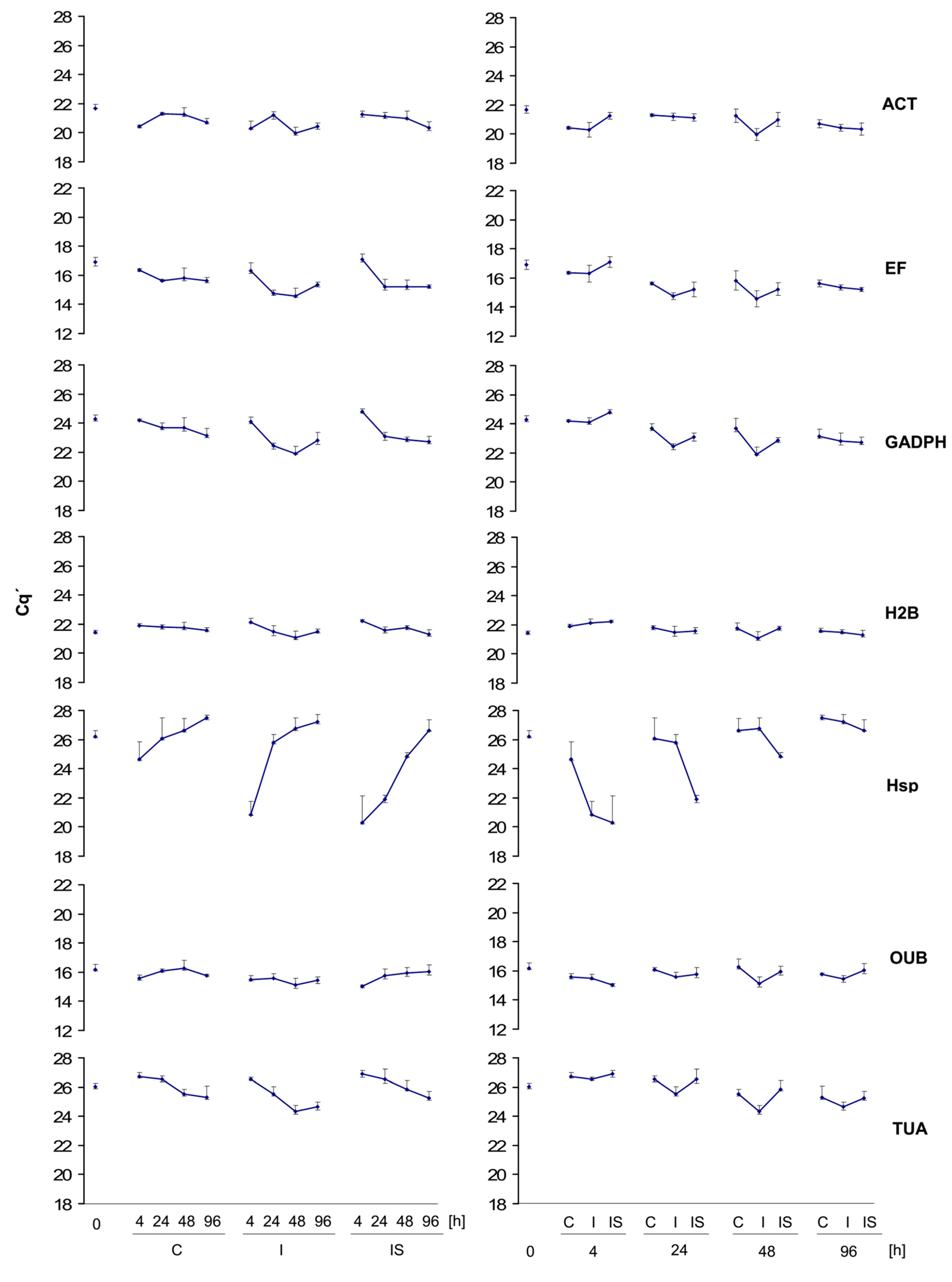
3.3.1. Displaying of Cq’ Means and Standard Deviation for Experimental Groups

The sample maximization design here used for plate arrangement avoids inter-run variability among samples, frequently underestimated [35]. Cq’ values for the amplicons of the seven CHGs were depicted (Figure 1) to allow a visual evaluation of the transcript level stabilities and common trends among genes along the different factors (time, treatment). Hsp resulted as the most unstable CHG, with a general opposite trend to ACT, EF, GAPPH, H2B and TUA, all of them genes showing a high degree of co-expression, v.g., co-regulation, in spite of they are functionally unrelated in a direct way. Co-regulation may be induced by stress or multi-stress [42,43], and could bias RG selection. In spite of their co-regulation, those genes show an opposite trend to the remaining and also stable gene, OUB, a behaviour that can be associated to its pre-proteolitic function, i.e., it is expressed when protein replacement is needed. The observed intra-group (time × treatment) variations were moderate except for Hsp, to what contributes a heterogeneous group-dependent variability among biological samples, since its intra-group inter-replicate variabilities were low (Figure 1).

3.3.2. Calculation of Transcriptional Gene Stability Values

CV and F statistics estimate, respectively, the overall and inter-group variation of transcript levels of single CHGs without counterbalancing with the rest of CHGs. Thus, CV and F estimators provide stability rankings which are unbiased by concomitant, systematic biological variations that may be associated with an experimental or assay condition, leading a group of genes following a similar expression trend, such as the variation due to co-regulation. Thus, CV and F provide, in most cases, a good classification of the stability of CHGs. It is worthwhile to point out that the purpose of CV and F statistics is the generation of a transcriptional gene stability ranking rather than gene transcriptional stability values, and not at all the obtaining of significant differences. Hence, inference statistics’ pre-requisites, such as normal distribution, are not mandatory for the pursued goal. F was calculated for bi- (time × treatment) and trifactorial (time × treatment × assay) cases (thus, F was referred to as F2 and F3, respectively).

3.4. Ranking of Candidate Housekeeping Genes According to Their Stability

The more transcriptionally stable genes should have a more or less parallel classification in both CV and F descriptive parameters [6]. In the CV/F method, preference is given to CV (overall variation) ranking [6], thereby overcoming possible large discrepancies caused by opposite and extreme values of CV and F. The rankings of CHGs, according to CV/F method—as well as rankings given by the other used software algorithms—are shown in

Table 3. Transcriptional stability rankings for transcript accumulation of candidate housekeeping genes for the whole panel of experimental conditions ^{1, 2}.

	All Replicates							Time × Treatment		Time × Treatment × Assay
	RFi Algorithms						CV	F2	Independent NFi	F3	Independent NFi
	BKr2	BKS	CoD	GNo	NFi	RFi
All tested housekeeping genes	EF (0.67)	H2B (0.34)	H2B (1.07)	EF/GAPDH (0.59)	OUB (0.24)	H2B (1.57)	H2B (0.29)	Hsp (4.84)	OUB (0.24)	H2B (11.66)	OUB (0.27)
	ACT (0.57)	OUB (0.38)	ACT (1.12)		H2B (0.32)	OUB (2.45)	OUB (0.34)	H2B (7.70)	H2B (0.26)	OUB (14.59)	H2B (0.28)
	OUB (0.55)	ACT (0.58)	OUB (1.14)	H2B (0.69)	ACT (0.38)	EF (2.83)	ACT (0.43)	OUB (8.49)	ACT (0.31)	ACT (26.05)	ACT (0.33)
	GAPDH (0.54)	EF (0.68)	EF (1.16)	TUA (0.74)	EF (0.66)	ACT (3.08)	EF (0.56)	ACT (10.79)	EF (0.45)	TUA (33.03)	EF (0.46)
	TUA (0.43)	GAPDH (0.76)	GAPDH (1.17)	ACT (0.79)	GAPDH (0.76)	GAPDH (3.34)	GAPDH (0.63)	EF (13.53)	GAPDH (0.49)	EF (34.86)	GAPDH (0.5)
	H2B (0.38)	TUA (0.80)	TUA (1.23)	OUB (0.82)	TUA (0.88)	TUA (5.42)	TUA (0.67)	TUA (17.89)	TUA (0.58)	GAPDH (38.6)	TUA (0.56)
	Hsp (0.30)	Hsp (2.01)	Hsp (2.79)	Hsp (1.38)	Hsp (2.74)	Hsp (7.00)	Hsp (3.04)	GAPDH (19.02)	Hsp (1.43)	Hsp (1237.12)	Hsp (1.37)
Best 6 tested housekeeping genes	EF (0.86)	H2B (0.34)	H2B (0.74)	EF/GAPDH(0.58)	H2B (0.42)	H2B (1.32)	H2B(0.29)	H2B (7.70)	H2B (0.21)	H2B (11.66)	H2B (0.21)
	GAPDH (0.85)	OUB (0.38)	GAPDH (0.80)		GAPDH (0.57)	GAPDH (2.11)	OUB (0.34)	OUB (8.49)	ACT (0.28)	OUB (14.59)	ACT (0.30)
	TUA (0.80)	ACT(0.58)	EF (0.82)	H2B (0.70)	EF (0.58)	EF (2.45)	ACT (0.43)	ACT (10.79)	EF (0.31)	ACT (26.05)	EF (0.32)
	H2B (0.64)	EF (0.68)	ACT (0.82)	TUA (0.74)	ACT (0.59)	ACT (3.94)	EF (0.56)	EF (13.53)	GAPDH (0.32)	TUA (33.03)	GAPDH (0.32)
	ACT (0.60)	GAPDH (0.76)	TUA (0.86)	ACT (0.79)	TUA (0.64)	OUB (4.56)	GAPDH (0.63)	TUA (17.89)	OUB (0.34)	EF (34.86)	OUB (0.36)
	OUB (0.37)	TUA (0.80)	OUB (0.88)	OUB (0.82)	OUB (0.70)	TUA (4.95)	TUA (0.67)	GAPDH (19.02)	TUA (0.37)	GAPDH (38.6)	TUA (0.37)

¹ According to BestKeeper Pearson coefficient of correlation (BKr) and the stability parameters for BestKeeper SD (BKS), comparative ΔCt method (CoD), GeNorm (GNo), NormFinder (NFi), RefFinfer (RFi) and CV/F method. A lower value for stability parameters (parentheses) indicates higher transcript accumulation stability. F and NF were calculated for different sample groups. Underlined are the genes contributing to the 2-genes normalization factor with maximum stability according to NFi independent software. In bold, genes selected as reference genes (see Figure 2). In cursive, the discarded CHG Hsp. ² All tested genes with p < 0.01 for Pearson correlation coefficient for the correspondent BestKeeper normalization factor, according to Pfaffl et al. (2004).

.

3.5. Discarding of Transcriptionally Unstable Genes

As is also evident from the visual distribution of CV and F parameters (Figure 1), Hsp resulted in a more transcriptionally unstable CHG for all methods used. Moreover, in Table 3, Hsp was ranked as the less stable CHG for CV and F3, and its first position in F2 was an effect of an intolerably high intra-group (inter-assay) Hsp instability. Consequently, Hsp was discarded and removed for subsequent re-rankings.

On the other hand, Hsp was highly overexpressed at 4 h, likely due to the stress caused by in vitro handling. This overexpression was greater in both treatments with IBA. Nevertheless, basal expression was progressively reached in all treatments after the initial stress was over. Thus, we decided to use Hsp 18.3 to validate the selected RGs.

3.6. Re-Rankings of Remaining Genes

For the CV/F method, the exclusion of Hsp did not change stability values nor the order of the rest of CHGs. Thus, omitting Hsp, the order of H2B, OUB, ACT and EF is clear for the CV/F method, and, taking into account the preference given to CV ranking over that of F, those genes may be followed by GAPDH and, finally, TUA. GAPDH showed the lowest inter-group stability according to both calculated F rankings, and had a relatively low score according to CV, being ranked 5th for this parameter.

3.7. Ranking with Software Methods as Support and Comparison with CV/F Ranking

The CHGs tested here (Table 3) were previously considered to be suitable RGs for in vitro plant growth and rooting studies ([8] and references therein) and are functionally distant. This last condition diminishes the risk that most of the CHG may be transcriptionally affected in a similar way by the experimental conditions. In spite of this, it has been advised that each individual CHG stability be evaluated by other means prior to the software usage [5]. CV has been used as a main parameter for normalization [44], sometimes complementing normalization software [6,45,46,47]. In other cases, the CV method has been used to compare with other methods to select the more adequate reference genes [48,49].

The software methods employed in the present study (except BKS algorithm implemented in RFi) use statistics that relate transcript levels among all used CHGs, and consequently rely on the hard-to-support assumption that a majority of the evaluated CHGs do not show real biological concomitant or systematic variations on their transcript accumulation between sample groups. In other words, in such software methods, the measured variation is assumed to be due to technical errors for most of the tested genes, i.e., all of those programs are sensitive to concomitant variations such as co-regulation [48], especially gNo and CoD [49,50]. Furthermore, NFi software, although less affected by co-regulation, does not account for inter-group systematic errors associated with sample preparation [50], in contrast to the use of F. On the other hand, BestKeeper requirements are too strict with the inter-sample variance [51]. Moreover, rankings offered by all of these methods are frequently conflicting ([6,7,10,30], reviewed in [9]). The RFi program uses the geometric mean of the other four software statistical approaches (BKS in the case of BestKeeper, and overall variation for NFi) to rank the CHGs. RFi [41] weighting may help to overcome some pitfalls, but it is obviously also influenced by the systematic variations affecting its integrated algorithms.

In spite of these commented pitfalls, with the exception of gNo, which the algorithm more strongly ranks according to similar gene transcript accumulation trends (likely a biasing effect), the rest of the software we employed agreed with the CV/F method in including H2B, OUB and ACT into the three or four firstly ranked CHGs. However, this was without concordance in the exact order positions (Table 3): H2B ranked from the 1st to 2nd position, OUB ranked the same (except for CoD method, where it ranked third), and ACT ranked between the 2nd and 4th positions. The remaining CHGs, in a sort of parallelism to the CV/F rank, usually oscillated between positions 3 and 5 (EF) or 4 and 6 (GAPDH and TUA), except in the case of gNo software, which considered EF and GAPDH as the optimal options.

The removal of the highly unstable Hsp affected the gene ranking obtained through methods for which transcript accumulation or Cq’ values of each CHG algorithmically interact with those from the others. Table 3 shows that H2B is still well ranked for all algorithms. Nonetheless, in those algorithms into RFi where the gene ranking is dependent on interactions between genes (CoD, gNo, and NFi), ACT and OUB pass into the last three positions. The removal of Hsp, which strongly affected average trends (see changes in BKr values), changed the rankings of CoD and gNo, two algorithms highly biased by co-regulation, which is a fact to consider, especially in cases of plant multi-stress induction (such as the present one) or even in cases of normally non co-regulated genes [42,43]. The NFi integrated into RFi is also sensible for inter-sample systematic variations: in the present case, it is sensible for co-regulation. The use of the remaining six CHGs for subsequent estimations reaches the limit of the advised number of CHGs to be used in a ranking algorithm NFi [36].

After Hsp removal, all methods showed H2B as the most stable CHG (or 3rd most stable for gNo) (Table 3). In other words, H2B is the only selected CHG common for all methods. H2B was previously recommended to be used as RG due to its high stability in in vitro rooted Eucalyptus globulus microcuttings [8]. ACT usually ranks between the 2nd and 4th positions. This ranking reinforces its 2nd place for CV/F. OUB, 3rd for CV/F ranking, is classified into the last two positions for those algorithms which are more susceptible to co-regulation effects. Since this is due to its transcript accumulation trend, opposite to the rest of the five remaining CHGs, in a way its behaviour compensates the opposite trend of both H2B and ACT, stabilizing the correspondent NF, as happens when the selection of two genes is configured for independent NFi. In this case, OUB transcript levels—together with H2B transcript levels—are suggested to compose the NF.

3.8. Selection of RG Sets

Selection of RGs composing NFs is performed after establishment of a stability ranking of CHGs. In spite of the commented preference for the CV/F method, in order to establish a stability ranking for CHGs, it is worthwhile to compare whether NFs obtained from each method can be similarly valid. There is a wide consensus on accepting different criteria for the establishment of a proper NF after CHG ranking, but they have not been applied together in a systematic way. According to the 2nd round of classifications (after discarding Hsp) of the prompted CHGs, such criteria were adapted for an optimal selection of RGs into each ranking methodology, as follows.

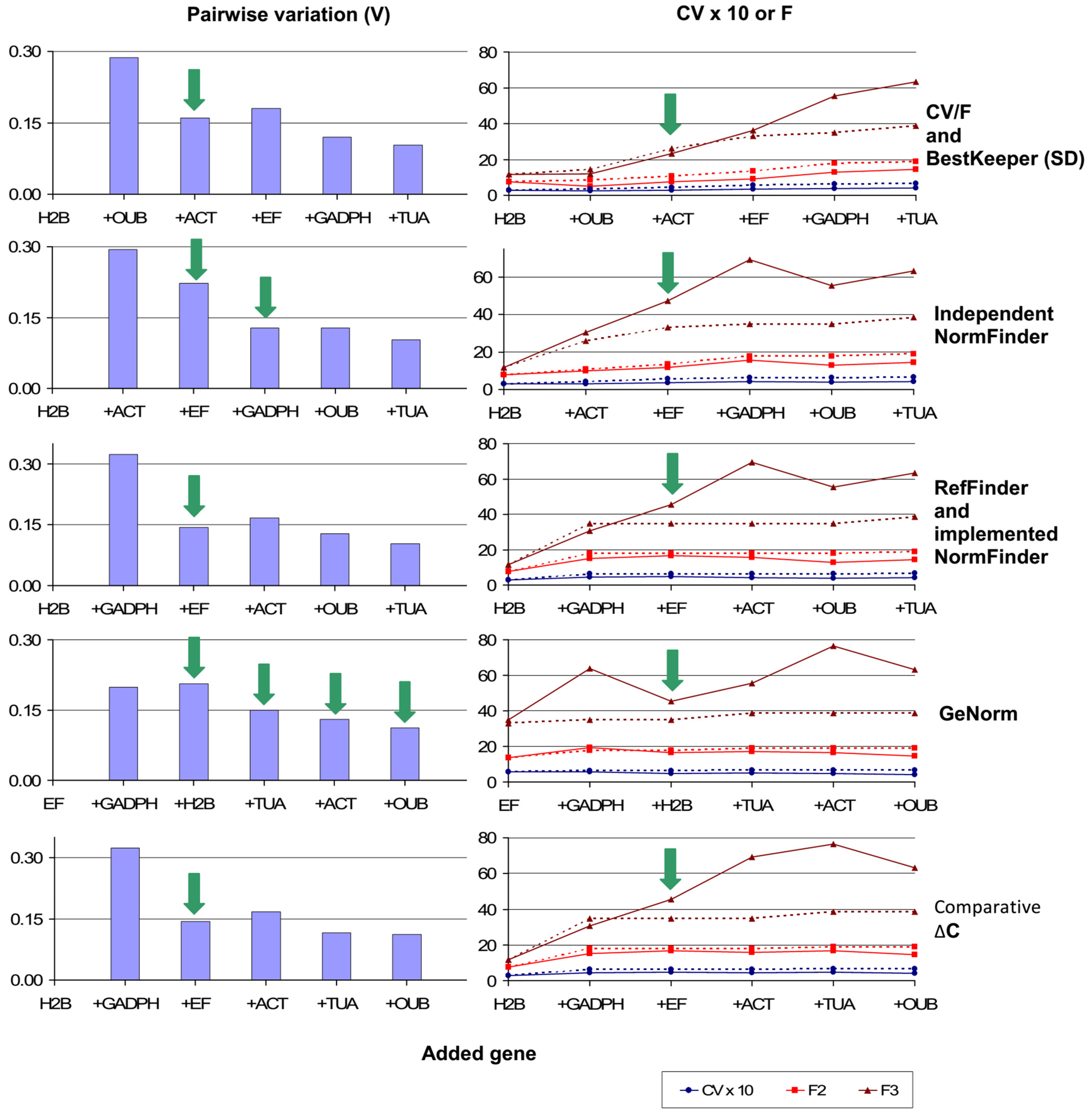
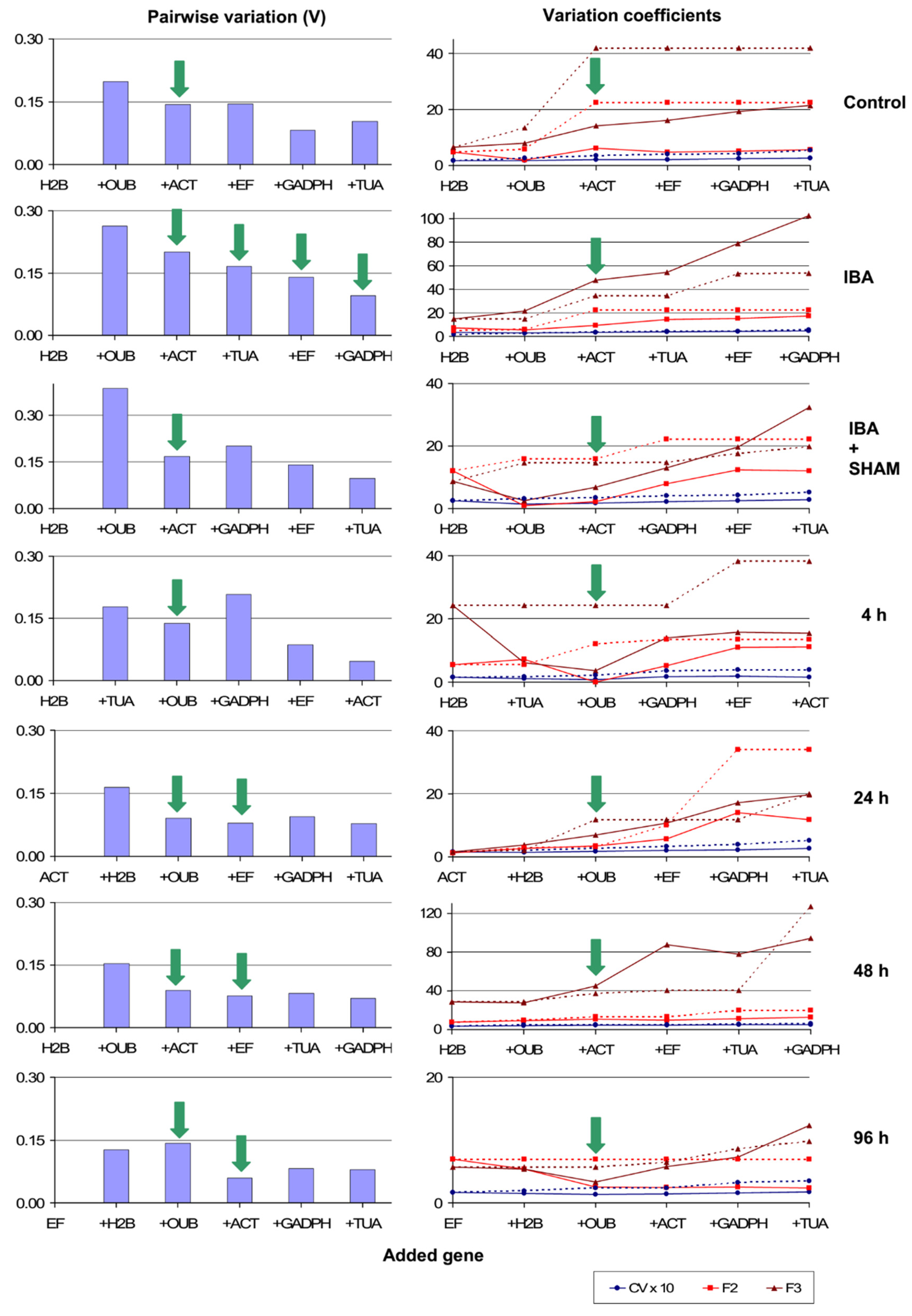
3.8.1. Calculation of Pairwise Variations between Possible NFs

A proper NF should be (i) as stable between samples as possible, as long as (ii) its variations mainly reflect the real technical errors in order that these errors be compensated for. The first criterion, NF stability, is usually procured through selection of a number of the most stable CHGs, i.e., RGs, the transcript levels of which compose the NF. According to this, six NFs were calculated for each gene ranking method, each NF being composed of the levels of the transcripts of the most stable n CHGs (n = 1 to 6) and ordered according to n (Figure 2).

The replicate pairwise variation (V) [24] indicates the variability between NF pairs. If V is low, both NFs are considered equivalent for normalization. If the compared NFs are composed each from the transcript levels of the n and the n + 1 most stable CHGs, and V is low, both NFs may be valid for normalization. If the pairwise comparisons are made from n = 1 to the total number of CHGs, the first low V found is considered to correspond to the optimal NF pair, and usually the NF composed from the transcript levels of the minor number of genes is selected. A V threshold value of 0.15 is accepted as low enough, but this consensus should not be strict [12], especially when considering complex designs of various factors, as in the case presented in this article. In addition, a trend of changing V values when adding new genes for the calculation of the NF is recognized to be equally informative [41,52,53], and, in fact, values higher than 0.15 have been accepted [42,54,55]. Concretely, the best option for a decreasing V trend are the NFs corresponding to the V lowest value. Moreover, if, after a decreasing trend, even to less than 0.15, V starts to grow again by the addition to the NF of a worse ranked CHG, more instability may be being introduced and, consequently, more error. Thus, the inclusion of such a CHG as RG is not advisable.

The methodology for V calculation has been used so far only for comparisons of pairs of NFs composed from the levels of n and n + 1 CHGs, as ranked according to the CHG stability obtained with gNo, since this algorithm is implemented in that software [24]. In the present work, such an algorithm was adapted to determine V between any pair of possible NFs, hereby obtaining the left graphics of Figure 2.

3.8.2. Determination of Representative Candidate NFs

Normalization against more than one gene is a priori recommended [56]. At least three RGs to calculate NF are recommendable [57,58]. Three non-physiologically related genes are more representative, as long as NF is stable.

3.8.3. Assessment of Congruent Stability and Selection of NFs for Each Gene Ranking Method

The selected NF between those constructed for each ranking method should be as stable as possible, as long as the previous criteria are kept. Maximum or high NF stability underlies the method proposed by [59] for choosing NFs, but this may overlook CHG representation. Thus, the overall CHG representation in the candidate NFs and the congruency of these NFs, according to the previous criteria of stability and compensation of errors, was tested by assessing the stability of the candidate NFs regarding discarded NFs and individual CHGs, a matter that tends to be overlooked. To inspect the suitability of the candidate NFs, the next rules were introduced:

• Ideally, important variability parameters (CV and F) for NFs should be lower than those of the CHG composing the NF, having the maximum values for such parameters (see Figure 2 right). Otherwise, this worse-ranked CHG may be unnecessarily contributing to additional NF instability.
• In this regard, as in general, when selecting NFs, the ranking provided by overall variability (CV) should ideally have priority over that given by inter-group variability (F).
• F would be more representative of the whole experimental panel if it spanned a higher number of factors: in the present case, F3 should have more priority than F2.
• Economic criteria may be additionally taken into account when two or more NFs may be similarly valid according to all above criteria, consequently selecting the RG set with the minimum number of CHGs.

In Table 3 (genes in bold) and Figure 2, the proposed and selected RGs (genes which contribute to the NFs) for different algorithms are represented after discarding Hsp as highly unstable gene and applying the above described criteria. In all cases, these rules brought NFs composed from the transcript levels of three RGs. Results showed three possible NFs, depending on the ranking method: H2B, OUB and ACT (for CV/F and BKS methods); H2B, ACT and EF (for independent NFi algorithms) and H2B, EF and GAPDH (for the rest of the methods). There is a consensus for the selection of these three CHGs amongst RFi and their implemented methods, except for BKS. This apparent congruence can be an effect of the bias by co-regulation. In the case of independent NFi, which takes into account biological groups, the GAPDH 2nd position resulting from those algorithms is substituted by ACT, but this can still be an effect of the influence of co-regulation. BKS and CV/F methods, which are not affected by the aforementioned pitfalls, change the ACT of the selected NF of independent NFi by OUB. The different trend of this gene, with respect to the majority of CHGs, increases the stability of the resulting NF. Only H2B, the most stable CHG for all methods except for gNo (where ranked 3rd), constituted a consensus between the selected NFs.

In order to test the possible validity of any of the three selected NFs, V values between them were calculated. V values were always much higher than 0.15 (0.27 was the lowest, data not shown); thus, there were important significant differences between the correspondent NFs. The commented deficiencies of algorithms suggest the CV/F method as a reasonable solution, at least as a first approach. Only BKS, which was unaffected by co-regulation since it uses a similar method to CV/F, had analogous results to CV classification. If one is not too strict with high standard deviation for BestKeeper, BKS classification could be a good combination with F to classify stable genes. In fact, according to [60], the BestKeeper approach may be useful for narrowing down a search if no specific genes are known to be plausible candidates.

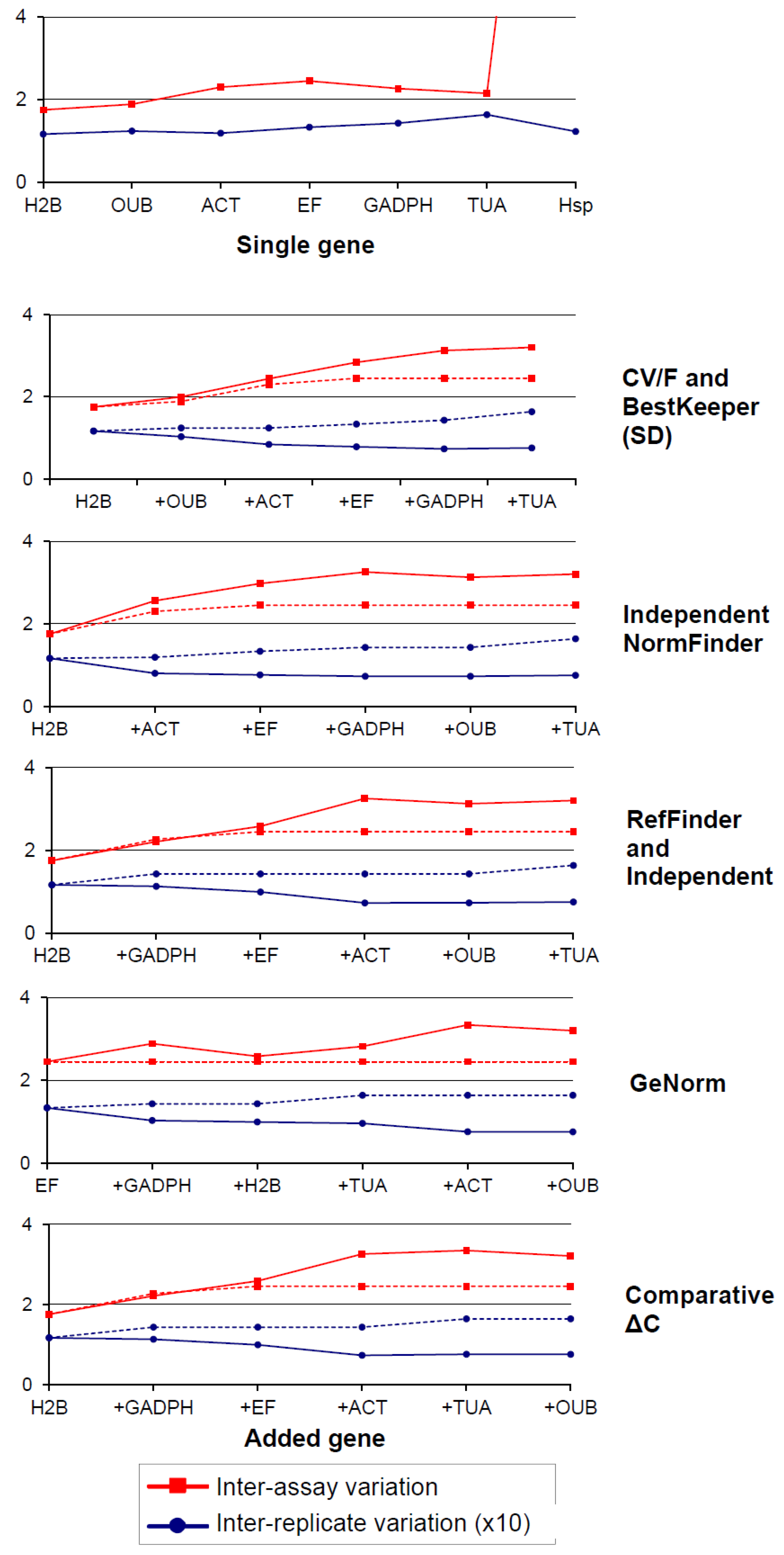
3.9. Error Compensation Versus Stability: Inspection of the Quality of the Selected NFs

The quality of NFs may be partially assessed by inspecting the following: (i) in what measure they compensate the technical errors of the measurements of transcript levels, and (ii) if they can also be valid for inter-assay (biological replicates in the present case) comparisons.

The total variation of the measurement of transcript levels comprises the real biological variation, plus technical errors. These last type of errors are systematic when they are due to experimental factors (e.g., in the case of samples from a given experimental condition, which are all more prone to RNA degradation), and may increase from the RNA isolation step onwards, due to associated effects such as carried-over effects (such as analytical processing of experimental groups at different times or in different conditions). Carried-over effects are minimized when using a sample maximization design [35], as in the present case, e.g., run-to-run variation. On the other hand, non-systematic, i.e., non-experimental condition-associated technical errors, should weigh proportionally less among experimental groups (formed by, for example, different treatments or time points) and should be processed more uniformly than among biological replicates if these are obtained from different assays. In the present case, since assay is a factor fixed by rooting potential, the assay-associated systematic variation (and consequently the included systematic error) should weigh proportionally more in the overall inter-assay variation than in assays for which the rooting potential would have been similar. Thus, in any case, the inter-assay systematic and technical errors should be compensated, as is possible by the selected NF avoiding the overcompensation, i.e., the compensation of the real biological inter-assay variation (i.e., inter-biological replicate variation). This convenience is kept for the NFs selected in the analyses (Figure 2) for all of the indicated CHG ranking methods, since inter-assay variation of these NFs is moderate or low with respect to the non-selected NFs and the individual CHGs (Figure 3). Furthermore, except for the independent NFi, the inter-assay variation of the selected NFs is similar to that of the CHG among those composing the NF, with maximal inter-assay variation. Thus, selection criterion i (Section 3.8) is also kept for the inter-assay case. These considerations lead to the conclusion that the selected NFs, for both bi- and trifactorial cases, are also valid for inter-assay comparisons (between biological samples with the same time × treatment).

Obviously, NFs should also compensate non-systematic analytical errors. The inter-technical replicate variation (Figure 3) virtually only accounts for the technical error accumulated during RT-replicates preparation and later associated effects, i.e., a non-systematic, non-experimental, factor-associated error. Inter-technical replicate variation tends to decrease asymptotically with the number of RGs to a theoretically precise average value, as is confirmed in Figure 3. In fact, all genes are absolutely stable for technical replicates, and, consequently, an inter-technical replicate error (variation) would be optimally compensated by a NF composed from the transcript levels of a large number of RGs. Nevertheless, the contribution to the NFs of such a large number of RGs would compromise other requirements, such as previously indicated criteria and good compensation for systematic errors, in this regard. Thus, a moderate NF inter-technical replicate variation value, which would, of course, be lower than the NF-composing CHG transcript levels with maximum value for this parameter, would be an acceptable deal. This is the case of the selected NFs. This indicates a partial compensation of inter-replicate error, without compromising systematic error compensations, and a reasonable stabilization of the NF.

The overall inter-technical replicate mean distance between Cq’s that would correspond to the NF composed from the transcript levels of all seven CHGs (Cq’ = 0.0042) specifically accounts for average error due to RT-replicate preparation. In exchange, the inter-technical replicate mean distances between Cq’s that would correspond to the selected NF should also include all non-systematic technical errors, either carried over or not. The selected NFs for each method are, again, well-ranked for this descriptor, having an intermediate-high value (0.0072 corrected cycles for the NF with three CHGs from CV/F, or similar for the rest of the selected NFs for each method), and, thus, overcompensating for the RT average error (0.0042 corrected cycles) and thereby accounting for later errors as well.

3.10. Determination of the Optimal Normalization Factor for the Complete Bi- and Trifactorial Panels

For the CV/F method, NF3, composed from the transcripts of H2B, OUB and ACT, is a good compromise to reduce V between two consecutive CHG groups (Figure 2). It has a more major representation than the NF composed from only two CHGs transcript levels (NF2), and retains the stability conditions stated above. OUB transcript levels have a slight opposite trend to both H2B and ACT transcript accumulations, compensating for bifactorial (time × treatment) and trifactorial (time × treatment × assay) inter-group variations for NF3. NF3 offers low inter-group (bi- or trifactorial) variation (Figure 2, right) and intermediate inter-technical replicate variation (Figure 3, right), thus being reasonably stable for group-associated systematic variations without compromising the compensation of non-systematic technical errors. The inclusion of additional genes (transcript levels) introduces more instability (Figure 2, right). Furthermore, the addition of the transcript levels of one or two worse-ranked genes is not advisable, since they are rarely selected when testing experimental conditions separately (see next Section). As a general conclusion, this three-gene NF (NF3) represents the optimal combination of CHG transcript levels amongst those tested for the general panel of assayed experimental conditions. Slight instability between groups for NF3 may account for systematic variations.

3.11. Normalization Factors for More Specific Experimental Conditions

Additionally, the validity of NF3 for specific treatments at a specific time point, and over time for a specific treatment, was checked. In these cases, the experimental condition groups consisted of the different levels of time or treatment (thus giving a one-factor design) or in combination with the assays (thus giving a two-factor design). Single CHGs were subjected to graphic inspection and ranked for each time or treatment according to the same algorithms used for the complete bi- or trifactorial panels (

Table 4. Stability rankings for transcript accumulation of candidate housekeeping gene for the indicated experimental conditions ¹.

	All Replicates (Treatment)						Time		Time × Assay
Level	BKS	CoD	GNo	NFi	RFi	CV	F	NFi	F	NFi
Control Treatment	H2B	ACT	ACT/ OUB	H2B	ACT (1.57)	H2B (0.18)	Hsp (3.85)	OUB (0.22)	H2B (6.6)	H2B (0.29)
	OUB	H2B		ACT	H2B (1.57)	OUB (0.26)	H2B (4.78)	H2B (0.26)	OUB (13.55)	OUB (0.29)
	ACT	OUB	H2B	OUB	OUB (2.06)	ACT (0.36)	OUB (5.86)	ACT (0.32)	EF (24.01)	ACT (0.3)
	EF	EF	EF	EF	EF (4.00)	EF (0.41)	GAPDH (7.27)	GAPDH (0.47)	GAPDH (27.98)	GAPDH (0.5)
	GAPDH	GAPDH	GAPDH	GAPDH	GAPDH (5.00)	GAPDH (0.42)	EF (8.93)	EF (0.5)	TUA (40.48)	EF (0.52)
	TUA	TUA	TUA	TUA	TUA (6.00)	TUA (0.54)	TUA (9.63)	TUA (0.64)	ACT (42.01)	TUA (0.62)
	Hsp	Hsp	Hsp	Hsp	Hsp (7.00)	Hsp (1.32)	ACT (22.53)	Hsp (1.01)	Hsp (442.64)	Hsp (1.08)
IBA	OUB	OUB	EF/GAPDH	OUB	OUB (1.32)	H2B (0.32)	OUB (5.51)	OUB (0.39)	OUB (13.16)	OUB (0.43)
	H2B	GAPDH		GAPDH	GAPDH (2.21)	OUB (0.34)	H2B (7.13)	H2B (0.44)	H2B (14.69)	H2B (0.44)
	ACT	H2B	OUB	H2B	H2B (2.91)	ACT (0.49)	ACT (12.54)	TUA (0.47)	TUA (29.5)	TUA (0.46)
	EF	TUA	H2B	TUA	EF (3.16)	TUA (0.62)	Hsp (12.54)	EF (0.48)	ACT (34.59)	EF (0.51)
	TUA	EF	TUA	EF	TUA (4.47)	EF (0.64)	EF (16.73)	ACT (0.49)	EF (53.02)	GAPDH (0.52)
	GAPDH	ACT	ACT	ACT	ACT (5.05)	GAPDH (0.67)	GAPDH (20.47)	GAPDH (0.49)	GAPDH (53.55)	ACT (0.53)
						Hsp (2.27)	TUA (24.77)		Hsp (2664.02)
IBA + SHAM	H2B	H2B	H2B/TUA	H2B	H2B (1.00)	H2B (0.25)	Hsp (4.04)	ACT (0.31)	H2B (8.68)	H2B (0.33)
	OUB	ACT		ACT	TUA (2.45)	OUB (0.32)	ACT (7.51)	H2B (0.34)	ACT (13.65)	ACT (0.34)
	ACT	TUA	ACT	TUA	ACT (2.45)	ACT (0.35)	TUA (8.69)	TUA (0.5)	OUB (14.68)	TUA (0.51)
	TUA	GAPDH	GAPDH	GAPDH	GAPDH (4.23)	GAPDH (0.42)	H2B (12.06)	GAPDH (0.53)	GAPDH (14.69)	GAPDH (0.51)
	GAPDH	EF	EF	EF	OUB (4.56)	EF (0.42)	EF (13.78)	EF (0.63)	EF (17.63)	EF (0.62)
	EF	OUB	OUB	OUB	EF (5.23)	TUA (0.53)	OUB (15.85)	OUB (0.66)	TUA (19.87)	OUB (0.67)
						Hsp (1.97)	GAPDH (22.17)		Hsp (1107.17)
4 h	GAPDH	GAPDH	EF|GAPDH	GAPDH	GAPDH (1.00)	H2B (0.16)	Hsp (3.19)	H2B (0.2)	TUA (4.11)	H2B (0.18)
	OUB	EF		TUA	EF (2.06)	TUA (0.18)	TUA (3.92)	GAPDH (0.2)	OUB (15.79)	GAPDH (0.22)
	EF	TUA	TUA	EF	TUA (2.91)	OUB (0.22)	EF (5.28)	TUA (0.2)	GAPDH (20.15)	EF (0.3)
	TUA	H2B	H2B	H2B	H2B (4.43)	GAPDH (0.25)	H2B (5.51)	EF (0.28)	EF (21.49)	TUA (0.3)
	ACT	ACT	ACT	ACT	OUB (4.56)	EF (0.37)	ACT (8.01)	ACT (0.33)	H2B (24.26)	ACT (0.35)
	H2B	OUB	OUB	OUB	ACT (5.00)	ACT (0.39)	OUB (12.15)	OUB (0.45)	ACT (38.25)	OUB (0.45)
						Hsp (1.53)	GAPDH (13.54)		Hsp (1408.8)
1 d	H2B	EF	EF|OUB	EF	EF (1.41)	ACT (0.15)	ACT (1.22)	EF (0.15)	ACT (1.58)	EF (0.22)
	ACT	OUB		OUB	OUB (1.86)	H2B (0.2)	H2B (2.85)	OUB (0.17)	H2B (1.98)	OUB (0.23)
	OUB	ACT	ACT	ACT	ACT (2.71)	OUB (0.27)	OUB (3.15)	H2B (0.25)	GAPDH (8.59)	H2B (0.27)
	EF	TUA	TUA	TUA	H2B (3.34)	EF (0.33)	TUA (7.6)	ACT (0.3)	EF (10.25)	ACT (0.32)
	GAPDH	H2B	H2B	H2B	TUA (4.43)	GAPDH (0.39)	EF (10.14)	TUA (0.31)	OUB (11.74)	TUA (0.37)
	TUA	GAPDH	GAPDH	GAPDH	GAPDH (5.73)	TUA (0.52)	GAPDH (34.04)	GAPDH (0.34)	TUA (20.03)	GAPDH (0.39)
						Hsp (1.19)	Hsp (145.76)		Hsp (41.6)
2d	H2B	H2B	ACT/OUB	H2B	H2B (1.32)	H2B (0.37)	EF (6.19)	OUB (0.19)	OUB (18.46)	H2B (0.23)
	OUB	OUB		OUB	OUB (1.68)	OUB (0.49)	H2B (7.79)	H2B (0.22)	H2B (28.88)	OUB (0.26)
	ACT	ACT	H2B	ACT	ACT (2.28)	ACT (0.52)	OUB (9.76)	EF (0.23)	TUA (33.74)	ACT (0.29)
	GAPDH	GAPDH	GAPDH	GAPDH	GAPDH (4)	EF (0.53)	ACT (13.31)	ACT (0.26)	ACT (37.23)	EF (0.35)
	TUA	EF	EF	EF	EF (5.23)	TUA (0.59)	GAPDH (17.13)	GAPDH (0.43)	EF (40.52)	GAPDH (0.37)
	EF	TUA	TUA	TUA	TUA (5.73)	GAPDH (0.61)	TUA (19.76)	TUA (0.49)	GAPDH (126.8)	TUA (0.46)
	Hsp	Hsp	Hsp	Hsp	Hsp (7.00)	Hsp (0.7)	Hsp (29.99)	Hsp (1.09)	Hsp (291.95)	Hsp (1.11)
4d	H2B	H2B	ACT/H2B	H2B	H2B (1.00)	EF (0.16)	GAPDH (1.21)	ACT (0.12)	OUB (4.12)	H2B (0.14)
	EF	ACT		ACT	ACT (2.00)	H2B (0.19)	H2B (2.16)	H2B (0.14)	H2B (5.36)	EF (0.21)
	OUB	EF	EF	EF	EF (2.71)	OUB (0.24)	ACT (2.29)	EF (0.15)	EF (5.66)	ACT (0.25)
	ACT	GAPDH	GAPDH	GAPDH	GAPDH (4.23)	ACT (0.24)	TUA (2.68)	GAPDH (0.21)	ACT (6.45)	GAPDH (0.35)
	GAPDH	OUB	OUB	OUB	OUB (4.4)	GAPDH (0.32)	Hsp (5.65)	OUB (0.32)	GAPDH (8.63)	OUB (0.4)
	TUA	TUA	TUA	TUA	TUA (6.00)	TUA (0.35)	EF (6.92)	TUA (0.34)	TUA (9.82)	TUA (0.44)
	Hsp	Hsp	Hsp	Hsp	Hsp (7.00)	Hsp (0.48)	OUB (6.99)	Hsp (0.37)	Hsp (33.83)	Hsp (0.5)

¹ According to stability parameters for BestKeeper SD (BKS), comparative ΔCt method (CoD), GeNorm (GNo), NormFinder (NFi), RefFinfer (RFi) and CV/F method, a lower value for stability parameters (parenthesis, indicated for RFi and algorithms non integrated in it) indicates higher transcript accumulation stability. Unstable genes were discarded. F and NFi were calculated for different sample groups. Underlined are the genes contributing to the 2-genes normalization factor with maximum stability, according to NFi independent software. Genes selected as reference genes are in bold (see Figure 4).

). After inspection of the graphics (Figure 1), Hsp, due to its high transcript accumulation instability, was removed from further consideration for the treatments IBA and IBA plus SHAM, and for the time points 4 h and 24 h. The genes ranked in last position for F were not removed for CV/F method, since they ranked in the first four positions according to CV (Table 4). After the determination of a CHG ranking according to the CV/F method, the method discussed above, in order to be considered, in general, more suitable, the previously described RG selection criteria were followed (Figure 4).

For a detailed selection of RGs for groups, see Table S1. To summarize (Figure 4), except for 96 h, where the combination for H2B, ACT and EF is the optimal, H2B and OUB transcript levels (NF2) belong to all selected NFs for the cases of specific experimental conditions (one given treatment with time point as a factor or a given time point with treatment as a factor), regardless of whether assay is included or not as a second factor. In some cases, the addition of transcript levels of EF (control treatment) or TUA (4 h) to NF2 forms the optimal set for normalization. In most cases (IBA, IBA and SHAM, 24 h and 48 h), the addition of ACT transcript levels to NF2 (and then constituting NF3) improves normalization according to the above pointed criteria. As previously indicated, for the bi- and trifactorial whole panels (treatment × time and treatment × time × assay, respectively), NF3 (H2B, OUB and ACT transcript levels) is proposed as the optimal NF.

For more specific cases (a given treatment at a given time point, or even biological or technical replicates in the same experimental conditions of the same assay), checking of the variability of CHGs between biological or technical replicates would be required, following a similar methodology to that here exposed. With the present transcript accumulation dataset, the total number of replicates inside of a given experimental condition (6 = 3 assays × 2 technical replicates) may be too low to perform a consistent test for those more specific cases. For this reason, if a NF must be estimated from the present datasets, the results obtained for the level-associated bifactorial cases (treatment level × assay or time level × assay) can be more valid. In spite of this, the decomposition of bi- and trifactorial whole panels for separate normalization and statistical comparison into the more simple level-associated mono- or bifactorial panels, respectively, is not advisable if a considerable loss of statistical power may be involved. Anyway, in such cases, CV and F values for NF3 are always low (data not shown), which supports the general use of NF3 as the most practical NF for most situations. Nevertheless, the obtained results coincide with those of other reports, where differences in RG stability depend on characteristics of biological material, environmental conditions or developmental stage ([5,61] and references therein). The complexity level of an experimental panel diminishes normalization accuracy, as can be expected a priori.

3.12. Evaluation of NF3 by Comparison with NF2

The proposition of NF3 as the best possible option for normalization of the whole panel was argued above (Section 3.10 and Section 3.11), as well as for several more concrete experimental conditions assayed herein. In spite of this, NF3 may be sub-optimal for the rest of the cases, and could be used as a less accurate solution. Nevertheless, according to the results on overall and intergroup variability for restricted panels (Figure 4), NF2 (which is like NF3, without including the transcript levels of the less stable gene, ACT), although less representative, could also constitute a good option, especially for more concrete experimental situations such as the monofactorial case of IBA and SHAM (Section 3.11). NF3 is evaluated below by comparison with NF2 while normalizing a hypothetical highly stable TG and a real TG with low stability, which is related to the stress caused by the experimental conditions. In this case, Hsp will serve as validation.

3.12.1. NF2/NF3 Comparison by Normalizing a Stable Target Gene

The theoretical results on an ideally completely stable TG (without any variation) regarding NF3 normalization were compared with those that would be obtained by normalizing the same TG with NF2. The results are equivalent to those achieved by normalizing NF3 against NF2, and they provide accurate differences between both NFs. Figure 5 shows the deviations (in marginal means of Cq’s) for such normalization after equalizing both NFs for time 0 (which constitutes the same situation for all treatments). Differences in marginal Cq’ means were only between 0.10 and 0.56, which are in the ranges of the intra-group standard deviations even of the more stable genes (Figure 1), thus indicating that normalization of a real stable gene (which would show intra-group standard deviations) with NF2 would easily reveal non-significant differences regarding NF3. In other words, in practice, NF2 or NF3 could be used for normalization of less stable genes without obtaining too many differences. In fact, the V for both NFs is approximately the threshold value of 0.15, which is accepted as low enough.

The obtained marginal Cq’ means are the log₂ of the equivalent transcript levels of F3 relative to those from F2, after equalization at time point 0. Since all marginal Cq’ means along time points are positive (Figure 5), normalization with NF3 will have lower relative transcript accumulation values for any TG other than those obtained using NF2. This may mean a slight overestimation of relative transcription levels if NF2 is used, in spite of the fact that these differences would generally be non-significant. According to the above justifications for adding a third RG to NF compositions, it is supposed that the introduction of ACT transcript levels into NF2 to compose NF3 corrects not only punctual non-systematic technical errors, but also some systematic, group-associated errors. Among these, a decrease in “NF2- equivalent transcript accumulation” can be detected 4 days after the experiment initiation or in samples from non-SHAM-treated explants (with stress palliated by AOX) 4 h after the experiment’s initiation. These can be inferred from Figure 5 (see caption).

3.12.2. NF2/NF3 Comparison and Validation by Normalizing an Unstable Gene

According to the previous conclusions, to evaluate the applicability of NF2 or NF3, significant differences in transcript levels of a real unstable gene (Hsp) were determined according to both NFs. As shown in Figure 1 and reflected in CV and F2 values (Table 3), Hsp displayed high bifactorial intragroup variation, but low bifactorial intergroup variation. Thus, the instability shown by Hsp is mainly associated with the intensity of the induced stresses, with a peak of transcripts at 4 h after induction. In order to perform ANOVAs, assumptions were tested using the Fligner–Killeen test, as well as graphics of residuals and observed and predicted values. When normalizing against NF2 and NF3, differences are obtained after Bonferroni transformation. These are shown in Table S2 and Figure S2. The use of NF3 renders lower calculated transcript levels than the use of NF2, as explained above, and thereby generates a small number of significant differences between groups, i.e., does not all of the differences generated by F2 in either bifactorial (time levels inside of treatment; eleven for NF2 and ten for NF3) or trifactorial(six for NF2 and five for NF3) cases. The other bifactorial case (treatment levels inside of time) showed a total of five significant differences for both NFs. Thus, globally, NF3 presented slightly more conservative results than NF2. To summarize, only inside of IBA and SHAM treatment, NF2 generated significant differences between 1d and 2d that NF3 did not (p =0.062), and the same occurred in BA for assays I and III.

3.12.3. Combined Evaluation

After applying both comparisons, it can be concluded that the more TG-transcript level variations appear (higher intra-group standard deviations and more evident inter-group variation), the fewer discrepancies regarding significant differences in gene transcript accumulation are generated by the application of different NFs. Thus, NF2, here considered as sub-optimal, can generate the same significant differences as NF3 when the TG is unstable enough, including when its expression depends on experimental conditions.

4. Conclusions

Selection of appropriate RGs is crucial for the validity of transcription studies. Different methods have been used to select reference genes in olive tissues [62,63,64,65], but never regarding the changes to the adventitious rooting process. The CV/F method (Section 3.3, Section 3.4, Section 3.5, Section 3.6 and Section 3.7) demonstrates a friendly and useful gene stability-ranking procedure, which lacks the inaccuracy generated by the influence of systematic errors, such as those generated by gene co-regulation. This inaccuracy may affect the most popular algorithms applied for such a purpose in different ways, leading to possible misinterpretations. Nevertheless, the additional use of popular software is advisable as complementary support for core methods. This is generally accepted knowledge of state-of-the-art methods. However, combining the criteria shown for selection of a proper number of stable RGs provides more accuracy for normalization. The nucleus of the integrated procedure is the selection of the RG sets (Section 3.8): (i) calculation of pairwise variations between any pair of possible proper NFs by implementing a method which, until now, has been used only when gNo software was run; (ii) determination of representative candidate NFs; and (iii) assessment of a congruent stability of candidate NF, a factor that is usually underconsidered.

The quality of the resulting NF may be additionally validated (Section 3.9) by inspecting its suitability for comparisons between non-considered factors or biological or technical replicates, as well as checking in what extension such NF compensate errors of transcript level measurement. For these purposes, special statistical estimators were formulated for the case currently in study.

The NF composed from the transcript levels of H2B, OUB and ACT provides a valid normalization for TGs in studies on olive microshoot adventitious rooting when comparing treatments, time points and assays (Section 3.10 and Section 3.11).

Finally, a double evaluation (Section 3.12) against both a theoretically highly stable gene and a real gene with relatively high instability provided information about the suitability of possible alternative NFs. The validity of the use of a sub-optimal NF depends on the variability of the studied TG. The more stable a TG is, the more transcript accumulation differences will be brought on by the application of different NFs.

References

1. Bustin, S.A. Quantitative Real-Time RT-PCR—A Perspective. J. Mol. Endocrinol. 2005, 34, 597–601. [Google Scholar] [CrossRef] [PubMed] [Green Version]
2. Wong, M.L.; Medrano, J.F. Real-Time PCR for MRNA Quantification. Biotechniques 2005, 39, 75–85. [Google Scholar] [CrossRef] [PubMed]
3. Huggett, J.; Dheda, K.; Bustin, S.; Zumla, A. Real-Time RT-PCR Normalisation; Strategies and Considerations. Genes Immun. 2005, 6, 279–284. [Google Scholar] [CrossRef] [PubMed] [Green Version]
4. Dundas, J.; Ling, M. Reference Genes for Measuring MRNA Expression. Theory Biosci. 2012, 131, 215–223. [Google Scholar] [CrossRef] [PubMed]
5. Joseph, J.T.; Poolakkalody, N.J.; Shah, J.M. Plant Reference Genes for Development and Stress Response Studies. J. Biosci. 2018, 43, 173–187. [Google Scholar] [CrossRef]
6. Kortner, T.M.; Valen, E.C.; Kortner, H.; Marjara, I.S.; Krogdahl, Å.; Bakke, A.M. Candidate Reference Genes for Quantitative Real-Time PCR (QPCR) Assays during Development of a Diet-Related Enteropathy in Atlantic Salmon (Salmo salar L.) and the Potential Pitfalls of Uncritical Use of Normalization Software Tools. Aquaculture 2011, 318, 355–363. [Google Scholar] [CrossRef]
7. Brunner, A.M.; Yakovlev, I.A.; Strauss, S.H. Validating Internal Controls for Quantitative Plant Gene Expression Studies. BMC Plant Biol. 2004, 4, 14. [Google Scholar] [CrossRef] [Green Version]
8. De Almeida, M.R.; Ruedell, C.M.; Ricachenevsky, F.K.; Sperotto, R.A.; Pasquali, G.; Fett-Neto, A.G. Reference Gene Selection for Quantitative Reverse Transcription-Polymerase Chain Reaction Normalization during in Vitro Adventitious Rooting in Eucalyptus Globulus Labill. BMC Mol. Biol. 2010, 11, 73. [Google Scholar] [CrossRef] [Green Version]
9. Kozera, B.; Rapacz, M. Reference Genes in Real-Time PCR. J. Appl. Genet. 2013, 54, 391–406. [Google Scholar] [CrossRef] [Green Version]
10. Torres, S.; Lama, C.; Mantecón, L.; Flemetakis, E.; Infante, C. Selection and Validation of Reference Genes for Quantitative Real-Time PCR in the Green Microalgae Tetraselmis Chui. PLoS ONE 2021, 16, e0245495. [Google Scholar] [CrossRef]
11. Zhu, L.; Yang, C.; You, Y.; Liang, W.; Wang, N.; MA, F.; Li, C. Validation of Reference Genes for QRT-PCR Analysis in Peel and Flesh of Six Apple Cultivars (Malus domestica) at Diverse Stages of Fruit Development. Sci. Hortic. 2019, 244, 165–171. [Google Scholar] [CrossRef]
12. Vandesompele, J.; De Preter, K.; Pattyn, F.; Poppe, B.; Van Roy, N.; De Paepe, A.; Speleman, F. GeNorm Software Manual. 2007. Available online: https://www.gene-quantification.com/geNorm_manual.pdf (accessed on 1 June 2022).
13. Salama, M.; Zahran, M.; Hassan, M. Comparing the Rooting Ability of Some Olive Cultivars Propagated by Leafy Cuttings under Mist. Ann. Agric Sci. Fac. Agric. Ain. Shams. Univ. 1987, 32, 577–590. [Google Scholar]
14. Qrunfleh, M.M.; Rushdi, Y.; Musmar, T.; Rushdi, L. Root Formation in Cuttings of “Nabali” Olives Treated with Uniconazole and Indole Butyric Acid. Dirasat 1994, 21, 71–79. [Google Scholar]
15. Fabbri, A. The Effect of Various Anatomical Characteristics on the Rooting of Cuttings in Olives, Cv. Frangivento. Riv. Della Ortoflorofruttic. Ital. 1980, 64, 325–335. [Google Scholar]
16. Bakr, E.; Selim, H.; Nour, G.; Gabr, M. Developmental Anatomy of Adventitious Roots on Stem Cuttings of “Wetaken” Olive Cultivar. Egypt. J. Hort. 1977, 4, 91–97. [Google Scholar]
17. Santos-Macedo, E.; Vieira, C.; Carrizo, D.; Porfirio, S.; Hegewald, H.; Arnholdt-Schmitt, B.; Calado, M.L.; Peixe, A. Adventitious Root Formation in Olive (Olea europaea L.) Microshoots: Anatomical Evaluation and Associated Biochemical Changes in Peroxidase and Polyphenol Oxidase Activities. J. Hortic. Sci. Biotechnol. 2013, 88, 53–59. [Google Scholar] [CrossRef]
18. Porfirio, S.; Calado, M.L.; Noceda, C.; Cabrita, M.J.; da Silva, M.G.; Azadi, P.; Peixe, A. Tracking Biochemical Changes during Adventitious Root Formation in Olive (Olea europaea L.). Sci. Hortic. 2016, 204, 41–53. [Google Scholar] [CrossRef] [Green Version]
19. Santos Macedo, E.; Sircar, D.; Cardoso, H.G.; Peixe, A.; Arnholdt-Schmitt, B. Involvement of Alternative Oxidase (AOX) in Adventitious Rooting of Olea europaea L. Microshoots Is Linked to Adaptive Phenylpropanoid and Lignin Metabolism. Plant Cell Rep. 2012, 31, 1581–1590. [Google Scholar] [CrossRef]
20. Arnholdt-Schmitt, B.; Costa, J.; de Melo, D. Alternative Respiration: Less Energy-Efficient but Highly Effective. Trends Plant Sci. 2006, 6, 281–287. [Google Scholar] [CrossRef]
21. Arnholdt-Schmitt, B.; Santos Macedo, E.; Peixe, A.; Cardoso, H.; Cordeiro, A. AOX—A Potential Functional Marker for Efficient Rooting in Olive Shoot Cuttings. In Proceedings of the Second International Seminar Olivebioteq, Marsala Mazara del Vallo, Italy, 5–10 November 2006; Volume 1, pp. 249–254. [Google Scholar]
22. Santos-Macedo, E.; Cardoso, H.; Hernández, A.; Peixe, A.; Polidoros, A.; Ferreira, A.; Cordeiro, A.; Arnholdt-Schmitt, B. Physiologic Responses and Gene Diversity Indicate Olive Alternative Oxidase as a Potential Source for Markers Involved in Efficient Adventitious Root Induction. Physiol. Plant. 2009, 137, 532–552. [Google Scholar] [CrossRef]
23. Peixe, A.; Serras, M.; Campos, C.; Zavattieri, M.; Dias, M. Adventitious Rooting in Olive (Olea europaea L.) Cuttings: A Histological Evaluation. Rev. Ciênc. Agrár. Soc. Ciênc. Agrár. Port. 2007, 30, 476–482. [Google Scholar]
24. Vandesompele, J.; De Preter, K.; Pattyn, F.; Poppe, B.; Van Roy, N.; De Paepe, A.; Speleman, F. Accurate Normalization of Real-Time Quantitative RT-PCR Data by Geometric Averaging of Multiple Internal Control Genes. Genome Biol. 2002, 3, RESEARCH0034. [Google Scholar] [CrossRef] [PubMed] [Green Version]
25. Ul Haq, S.; Khan, A.; Ali, M.; Khattak, A.M.; Gai, W.X.; Zhang, H.X.; Wei, A.M.; Gong, Z.H. Heat Shock Proteins: Dynamic Biomolecules to Counter Plant Biotic and Abiotic Stresses. Int. J. Mol. Sci. 2019, 20, 5321. [Google Scholar] [CrossRef] [PubMed] [Green Version]
26. Abbas, A.; Yu, H.; Li, X.; Cui, H.; Chen, J.; Huang, P. Selection and Validation of Reference Genes for RT-QPCR Analysis in Aegilops Tauschii (Coss.) under Different Abiotic Stresses. Int. J. Mol. Sci. 2021, 22, 11017. [Google Scholar] [CrossRef]
27. Chen, J.; Huang, Z.; Huang, H.; Wei, S.; Liu, Y.; Jiang, C.; Zhang, J.; Zhang, C. Selection of Relatively Exact Reference Genes for Gene Expression Studies in Goosegrass (Eleusine indica) under Herbicide Stress. Sci. Rep. 2017, 7, 46494. [Google Scholar] [CrossRef]
28. Wang, B.; Duan, H.; Chong, P.; Su, S.; Shan, L.; Yi, D.; Wang, L.; Li, Y. Systematic Selection and Validation of Suitable Reference Genes for Quantitative Real-Time PCR Normalization Studies of Gene Expression in Nitraria Tangutorum. Sci. Rep. 2020, 10, 15891. [Google Scholar] [CrossRef]
29. Nicot, N.; Hausman, J.-F.; Hoffmann, L.; Evers, D. Housekeeping Gene Selection for Real-Time RT-PCR Normalization in Potato during Biotic and Abiotic Stress. J. Exp. Bot. 2005, 56, 2907–2914. [Google Scholar] [CrossRef]
30. Zhang, L.; Zhang, Q.-L.; Wang, X.-T.; Yang, X.-Z.; Li, X.-P.; Yuan, M.-L. Selection of Reference Genes for QRT-PCR and Expression Analysis of High-Altitude-Related Genes in Grassland Caterpillars (Lepidoptera: Erebidae: Gynaephora) along an Altitude Gradient. Ecol. Evol. 2017, 7, 9054–9065. [Google Scholar] [CrossRef]
31. Ashish, S.; Bhure, S.K.; Harikrishna, P.; Ramteke, S.S.; Muhammed Kutty, V.H.; Shruthi, N.; Ravi Kumar, G.V.P.P.S.; Manish, M.; Ghosh, S.K.; Mihir, S. Identification and Evaluation of Reference Genes for Accurate Gene Expression Normalization of Fresh and Frozen-Thawed Spermatozoa of Water Buffalo (Bubalus bubalis). Theriogenology 2017, 92, 6–13. [Google Scholar] [CrossRef]
32. Nardeli, S.M.; Matta, B.P.; Saad, C.F.; Reinert, F.; Peixoto, R.S.; Alves-Ferreira, M. Early Heat Shock Protein Response and Selection of Reference Genes in Arabidopsis Thaliana Seedlings Subjected to Marine Fuel Contamination. Water Air Soil Pollut. 2017, 228, 101. [Google Scholar] [CrossRef]
33. Assab, E.; Rampino, P.; Mita, G.; Perrotta, C. Heat Shock Response in Olive (Olea europaea L.) Twigs: Identification and Analysis of a CDNA Coding a Class I Small Heat Shock Protein. Plant Biosyst. Int. J. Deal. All Asp. Plant Biol. 2011, 145, 419–425. [Google Scholar] [CrossRef]
34. Sambrook, J.; Fritsch, E.; Maniatis, T. Molecular Cloning. In A Laboratory Manual, 4th ed.; Cold Spring Harbor Laboratory Press: Cold Spring Harbor, NY, USA, 2012. [Google Scholar]
35. Hellemans, J.; Mortier, G.; De Paepe, A.; Speleman, F.; Vandesompele, J. QBase Relative Quantification Framework and Software for Management and Automated Analysis of Real-Time Quantitative PCR Data. Genome Biol. 2007, 8, R19. [Google Scholar] [CrossRef] [PubMed] [Green Version]
36. Andersen, C.; Jensen, J.; Ørntoft, T. Normalization of Real-Time Quantitative Reverse Transcription-PCR Data: A Model-Based Variance Estimation Approach to Identify Genes Suited for Normalization, Applied to Bladder and Colon Cancer Data Sets. Cancer Res. 2004, 64, 5245–5250. [Google Scholar] [CrossRef] [PubMed] [Green Version]
37. Walker, N. A Technique Whose Time Has Come. Science 2002, 296, 557–559. [Google Scholar] [CrossRef]
38. Ruijter, J.M.; Ramakers, C.; Hoogaars, W.M.H.; Karlen, Y.; Bakker, O.; van den Hoff, M.J.B.; Moorman, A.F.M. Amplification Efficiency: Linking Baseline and Bias in the Analysis of Quantitative PCR Data. Nucleic Acids Res. 2009, 37, e45. [Google Scholar] [CrossRef]
39. Pfaffl, M.W.; Tichopad, A.; Prgomet, C.; Neuvians, T.P. Determination of Stable Housekeeping Genes, Differentially Regulated Target Genes and Sample Integrity: BestKeeper--Excel-Based Tool Using Pair-Wise Correlations. Biotechnol. Lett. 2004, 26, 509–515. [Google Scholar] [CrossRef]
40. Silver, N.; Best, S.; Jiang, J.; Thein, S.L. Selection of Housekeeping Genes for Gene Expression Studies in Human Reticulocytes Using Real-Time PCR. BMC Mol. Biol. 2006, 7, 33. [Google Scholar] [CrossRef] [Green Version]
41. Hu, R.; Fan, C.; Li, H.; Zhang, Q.; Fu, Y.-F. Evaluation of Putative Reference Genes for Gene Expression Normalization in Soybean by Quantitative Real-Time RT-PCR. BMC Mol. Biol. 2009, 10, 93. [Google Scholar] [CrossRef] [Green Version]
42. De Jonge, H.J.M.; Fehrmann, R.S.N.; de Bont, E.S.J.M.; Hofstra, R.M.W.; Gerbens, F.; Kamps, W.A.; de Vries, E.G.E.; van der Zee, A.G.J.; te Meerman, G.J.; ter Elst, A. Evidence Based Selection of Housekeeping Genes. PLoS ONE 2007, 2, e898. [Google Scholar] [CrossRef] [Green Version]
43. Boda, E.; Pini, A.; Hoxha, E.; Parolisi, R.; Tempia, F. Selection of Reference Genes for Quantitative Real-Time RT-PCR Studies in Mouse Brain. J. Mol. Neurosci. 2009, 37, 238–253. [Google Scholar] [CrossRef]
44. Zampieri, M.; Ciccarone, F.; Guastafierro, T.; Bacalini, M.; Calabrese, R.; Moreno-Villanueva, M.; Realea, A.; Chevannec, M.; Bürkleb, A.; Caiafa, P. Validation of Suitable Internal Control Genes for Expression Studies in Aging. Mech. Ageing Dev. 2010, 131, 79–85. [Google Scholar] [CrossRef] [PubMed] [Green Version]
45. Sundaram, V.K.; Sampathkumar, N.K.; Massaad, C.; Grenier, J. Optimal Use of Statistical Methods to Validate Reference Gene Stability in Longitudinal Studies. PLoS ONE 2019, 14, e0219440. [Google Scholar] [CrossRef] [PubMed] [Green Version]
46. Khanlou, K.M.; van Bockstaele, E. A Critique of Widely Used Normalization Software Tools and an Alternative Method to Identify Reliable Reference Genes in Red Clover (Trifolium pratense L.). Planta 2012, 236, 1381–1393. [Google Scholar] [CrossRef] [PubMed]
47. de Santis, C.; Smith-Keune, C.; Jerry, D.R. Normalizing RT-QPCR Data: Are We Getting the Right Answers? An Appraisal of Normalization Approaches and Internal Reference Genes from a Case Study in the Finfish Lates Calcarifer. Mar. Biotechnol. 2011, 13, 170–180. [Google Scholar] [CrossRef]
48. Zsóri, K.; Muszbek, L.; Csiki, Z.; Shemirani, A. Validation of Reference Genes for the Determination of Platelet Transcript Level in Healthy Individuals and in Patients with the History of Myocardial Infarction. Int. J. Mol. Sci. 2013, 14, 3456–3466. [Google Scholar] [CrossRef]
49. Axtner, J.; Sommer, S. Validation of Internal Reference Genes for Quantitative Real-Time PCR in a Non-Model Organism, the Yellow-Necked Mouse, Apodemus Flavicollis. BMC Res. Notes 2009, 2, 264. [Google Scholar] [CrossRef] [Green Version]
50. Goulao, L.; Fortunato, A.; Ramalho, J. Selection of Reference Genes for Normalizing Quantitative Real-Time PCR Gene Expression Data with Multiple Variables in Coffea Spp. Plant Mol. Biol. Rep. 2012, 30, 741–759. [Google Scholar] [CrossRef]
51. Le, D.T.; Aldrich, D.L.; Valliyodan, B.; Watanabe, Y.; van Ha, C.; Nishiyama, R.; Guttikonda, S.K.; Quach, T.N.; Gutierrez-Gonzalez, J.J.; Tran, L.S.P.; et al. Evaluation of Candidate Reference Genes for Normalization of Quantitative RT-PCR in Soybean Tissues under Various Abiotic Stress Conditions. PLoS ONE 2012, 7, e46487. [Google Scholar] [CrossRef]
52. Reid, K.E.; Olsson, N.; Schlosser, J.; Peng, F.; Lund, S.T. An Optimized Grapevine RNA Isolation Procedure and Statistical Determination of Reference Genes for Real-Time RT-PCR during Berry Development. BMC Plant Biol. 2006, 6, 27. [Google Scholar] [CrossRef] [Green Version]
53. Hong, S.Y.; Seo, P.J.; Yang, M.S.; Xiang, F.; Park, C.M. Exploring Valid Reference Genes for Gene Expression Studies in Brachypodium Distachyon by Real-Time PCR. BMC Plant Biol. 2008, 8, 112. [Google Scholar] [CrossRef] [Green Version]
54. Maroufi, A.; Van Bockstaele, E.; De Loose, M. Validation of Reference Genes for Gene Expression Analysis in Chicory (Cichorium intybus) Using Quantitative Real-Time PCR. BMC Mol. Biol. 2010, 11, 15. [Google Scholar] [CrossRef] [PubMed] [Green Version]
55. Marum, L.; Miguel, A.; Ricardo, C.P.; Miguel, C. Reference Gene Selection for Quantitative Real-Time PCR Normalization in Quercus Suber. PLoS ONE 2012, 7, e35113. [Google Scholar] [CrossRef]
56. Bustin, S.A.; Benes, V.; Garson, J.A.; Hellemans, J.; Huggett, J.; Kubista, M.; Mueller, R.; Nolan, T.; Pfaffl, M.W.; Shipley, G.L.; et al. The MIQE Guidelines:Minimum Information for Publication of Quantitative Real-Time PCR Experiments. Clin. Chem. 2009, 55, 611–622. [Google Scholar] [CrossRef] [PubMed] [Green Version]
57. Bustin, S.A.; Beaulieu, J.-F.; Huggett, J.; Jaggi, R.; Kibenge, F.S.B.; Olsvik, P.A.; Penning, L.C.; Toegel, S. MIQE Précis: Practical Implementation of Minimum Standard Guidelines for Fluorescence-Based Quantitative Real-Time PCR Experiments. BMC Mol. Biol. 2010, 11, 74. [Google Scholar] [CrossRef] [Green Version]
58. Derveaux, S.; Vandesompele, J.; Hellemans, J. How to Do Successful Gene Expression Analysis Using Real-Time PCR. Methods 2010, 50, 227–230. [Google Scholar] [CrossRef]
59. Chervoneva, I.; Li, Y.; Schulz, S.; Croker, S.; Wilson, C.; Waldman, S.A.; Hyslop, T. Selection of Optimal Reference Genes for Normalization in Quantitative RT-PCR. BMC Bioinform. 2010, 11, 253. [Google Scholar] [CrossRef] [Green Version]
60. Lyng, M.B.; Laenkholm, A.-V.; Pallisgaard, N.; Ditzel, H.J. Identification of Genes for Normalization of Real-Time RT-PCR Data in Breast Carcinomas. BMC Cancer 2008, 8, 20. [Google Scholar] [CrossRef] [Green Version]
61. Wan, Q.; Chen, S.; Shan, Z.; Yang, Z.; Chen, L.; Zhang, C.; Yuan, S.; Hao, Q.; Zhang, X.; Qiu, D.; et al. Stability Evaluation of Reference Genes for Gene Expression Analysis by RT-QPCR in Soybean under Different Conditions. PLoS ONE 2017, 12, e0189405. [Google Scholar] [CrossRef] [Green Version]
62. Nonis, A.; Vezzaro, A.; Ruperti, B. Evaluation of RNA Extraction Methods and Identification of Putative Reference Genes for Real-Time Quantitative Polymerase Chain Reaction Expression Studies on Olive (Olea europaea L.) Fruits. J. Agric. Food Chem. 2012, 60, 6855–6865. [Google Scholar] [CrossRef]
63. Resetic, T.; Stajner, N.; Bandelj, D.; Javornik, B.; Jakse, J. Validation of Candidate Reference Genes in RT-QPCR Studies of Developing Olive Fruit and Expression Analysis of Four Genes Involved in Fatty Acids Metabolism. Mol. Breed. 2013, 32, 211–222. [Google Scholar] [CrossRef]
64. Ray, D.L.; Johnson, J.C. Validation of Reference Genes for Gene Expression Analysis in Olive (Olea europaea) Mesocarp Tissue by Quantitative Real-Time RT-PCR. BMC Res. Notes 2014, 7, 304. [Google Scholar] [CrossRef] [PubMed] [Green Version]
65. Hürkan, K.; Sezer, F.; Özbilen, A.; Taşkın, K.M. Identification of Reference Genes for Real-Time Quantitative Polymerase Chain Reaction Based Gene Expression Studies on Various Olive (Olea europaea L.) Tissues. J. Hortic. Sci. Biotechnol. 2018, 93, 644–651. [Google Scholar] [CrossRef]
Figure 1. Corrected quantification cycle (Cq’) values for the seven candidate housekeeping genes. Mean of biological replicates is represented, with upper semi-bars indicating Cq’ SD for biological × technical replicates (n = 6 = 3 assays × 2 RT-level replicates), and bottom semi-bars indicating Cq’ mean of SD of each biological replicate (3 assays with 2 RT-level replicates each). Blue lines connect time points insede of a treatment or treatments inside a time point.
Agronomy 12 03201 g001
Figure 2. Pairwise variation (left graphics) and descriptive parameters (right graphics) for the normalization factors (NFs). NFs are composed from the transcript levels of the indicated candidate housekeeping genes (consecutively included in the NF from the left to the right side of x axis), and determined according to the indicated methods (right column labels). Descriptive parameters are CV and F for bifactorial (F2) and trifactorial (F3) cases. Dotted lines indicate the maximum values of the parameter of the candidate housekeeping genes, which transcript levels contribute to the indicated NFs. Green arrows indicate the selected NFs after the determination of representative candidate NFs (left graphics) and the assessment of congruent stability (right graphics) (see text, Section 3.8).
Agronomy 12 03201 g002
Figure 3. Error compensation and stability of normalization factors. Inter-assay and inter-technical replicate variations for candidate housekeeping genes (upper graph) the normalization factors (NFs) composed from the indicated candidate housekeeping genes (consecutively included in the NF from the left to the right side of x axis), obtained according to the indicated methods (right column labels). Dotted lines show the maximum values of the indicated parameters into the candidate housekeeping genes, contributing to the indicated NFs.
Agronomy 12 03201 g003
Figure 4. Pairwise variation (left graphics) and descriptive parameters (right graphics) for the normalization factors (NFs) at the indicated time points (left labels). NFs are composed of the transcript levels of the indicated candidate housekeeping genes (consecutively included in the NF from the left to right side of X axis), and determined for CV ranking. Descriptive parameters are CV and F for bifactorial (F2) and trifactorial (F3) cases. Dotted lines indicate the maximum value of the parameter of the CHGs, transcript levels of which contribute to the indicated NFs. Green arrows indicate the selected NFs after the determination of representative candidate NFs (left graphics) and the assessment of congruent stability (right graphics) (see text, Section 3.8).
Agronomy 12 03201 g004
Figure 5. Estimated marginal Cq’ means obtained after normalizing NF3 with NF2, along different time points (hours). The obtained marginal Cq’ means are the log2 of the equivalent transcript levels of NF3 relative to those from NF2, after equalization of both NFs at time point 0. The equivalent transcript levels of NF2 relative to those from F3 would follow an opposite, specular trend. NF3: normalization factor composed from H2B, OUB and ACT transcript levels. NF2: normalization factor composed from H2B and OUB transcript levels. Significant differences in time points, treatments or assays are indicated by different lowercase letters, capital letters or romans, respectively.
Agronomy 12 03201 g005