Article

Mapping of Soil pH Based on SVM-RFE Feature Selection Algorithm

1
Academy of Digital China (Fujian), Fuzhou University, Fuzhou 350108, China
2
Department of Geography, Minjiang University, Fuzhou 350108, China
3
Technology Innovation Center for Monitoring and Restoration Engineering of Ecological Fragile Zone in Southeast China, MNR, Fuzhou 350108, China
*
Authors to whom correspondence should be addressed.
Agronomy 2022, 12(11), 2742; https://doi.org/10.3390/agronomy12112742
Submission received: 12 September 2022 / Revised: 19 October 2022 / Accepted: 1 November 2022 / Published: 4 November 2022
(This article belongs to the Special Issue Soil Sustainability in the Anthropocene)

Abstract

:
The explicit mapping of spatial soil pH is beneficial to evaluate the effects of land-use changes in soil quality. Digital soil mapping methods based on machine learning have been considered one effective way to predict the spatial distribution of soil parameters. However, selecting optimal environmental variables with an appropriate feature selection method is key work in digital mapping. In this study, we evaluated the performance of the support vector machine recursive feature elimination (SVM-RFE) feature selection methods with four common performance machine learning methods in predicting and mapping the spatial soil pH of one urban area in Fuzhou, China. Thirty environmental variables were collected from the 134 samples that covered the entire study area for the SVM-RFE feature selection. The results identified the five most critical environmental variables for soil pH value: mean annual temperature (MAT), slope, Topographic Wetness Index (TWI), modified soil-adjusted vegetation index (MSAVI), and Band5. Further, the SVM-RFE feature selection algorithm could effectively improve the model accuracy, and the extreme gradient boosting (XGBoost) model after SVM-RFE feature selection had the best prediction results (R2 = 0.68, MAE = 0.16, RMSE = 0.26). This paper combines the RFE-SVM feature selection with machine learning models to enable the fast and inexpensive mapping of soil pH, providing new ideas for predicting soil pH at small and medium scales, which will help with soil conservation and management in the region.

1. Introduction

Soil acidification is one of the most serious environmental issues globally [1]. More than 30% of soil worldwide is becoming acidic due to intensive anthropogenetic activities. pH is the key to detecting changes in soil acidification or soil alkalinity. Strong associated relationships have been proved between soil pH and soil quality, e.g., physical structure and microorganism structure, crop yields via impacting the effectiveness of nutrients, and soil health, e.g., the buffer capacity in the heavy metal [2]. Furthermore, pH is also affected by natural and anthropogenic factors, e.g., climate, soil type, soil-forming parent material, land use, vegetation cover, topography, and agricultural activities [3,4,5,6]. Therefore, spatial pH variation is essential for monitoring regional soil quality and land use.
Traditional and digital soil mapping methods for soil pH are the two ways to predict the soil spatial distribution. The first method needs to be completed through data collection, indoor prediction, field investigation, indoor interpretation, field check, and demarcation mapping [7]. The second method is the soil-landscape model [8]. This method can utilize the observed data to determine the spatial distribution of the soil properties. Further, this method has significantly increased spatial information authenticity and accuracy with an electronic graphical expression [9]. This method needs less money and time and can significantly improve prediction accuracy [10]. For example, Cai et al. [11] used three modeling methods, partial least squares regression, support vector machine regression, and random forest, to develop hyperspectral inversion models of soil pH. Dharumarajan et al. [12] used a random forest model to predict soil pH in a semi-arid tropical region of southern India. Rad [13] also used a random forest model to study spatial variability and predict the soil pH mapping in eastern Iran’s floodplains. In addition, regression methods have been commonly applied in digital soil mapping [14,15], such as the general linear regression method, partial least squares method, and geo-weighted regression method. Recently, machine learning models have been utilized generally due to their high performance in prediction for the non-linear relationships between soil properties and environmental variables.
The key to better predicting spatial soil pH is selecting appropriate environmental factors. Based on the previous studies, the main common environmental variables influencing soil pH can be divided into five categories: climate, remote sensing bands, vegetation index, land-use types, and topography. Research has shown that climatic factors influence soil pH [16]. Temperature can affect the soil pH by changing the soil microbial activity and moisture content [17]. The leaching of rainfall can lead to the loss of alkaline material from the soil, reducing the soil’s buffering capacity to acids, gradually forming exchangeable soil acids, and altering soil pH [18]. In recent years, multi-source remote sensing images have been applied to predict soil pH due to the wide detection range and data acquisition. It can be predicted by the strong response of visible, near-infrared, and short-wave infrared bands of multi-source remote sensing images [19,20]. Furthermore, the vegetation indices induced from multi-source remote sensing image bands as biological variables have responded well to soil pH changes [21]. In addition, as one comprehensive reflection of human land-use activities, land use is often closely related to soil pH [22]. Because land-use changes can have an effect on improving the soil structure, strengthening soil resistance, and maintaining and improving soil quality [23], elevation, slope, aspect, and other topographic features can affect the soil and parent material differently under varied lighting, water, and diving circumstances, frequently resulting in a regional variance in soil pH [24,25].
However, finding the optimal environmental variables with better model performance is a key step in digital soil mapping [26]. Therefore, selecting environments with a strong correlation with soil properties as auxiliary variables for the model is a crucial issue, and feature selection in machine learning can effectively address this problem. For example, Zhao et al. [27] used differential evolutionary feature selection and principal component analysis to invert the surface soil moisture of agricultural fields. Their results indicated that the model’s accuracy was improved after feature selection. Zeraatpisheh et al. [28] used the Boruta feature selection method to select different environmental datasets to predict soil organic carbon in Iranian arid agroecosystems. The results showed that the accuracy of the models built with additional data sets varied. Feature selection is essential for shortening the model running time and improving the model accuracy, and the optimal feature set should be selected for modeling.
Therefore, in this study, thirty environmental variables, including climatic factors, remote sensing images, vegetation index, digital elevation model (DEM) derivatives, soil properties, and human factors, were used to develop a soil pH prediction model by combining the support vector machine recursive feature elimination (SVM-RFE) feature selection method with different machine learning models. The aims of this study were to: (1) evaluate the performance of SVM-RFE feature selection methods combined with different machine learning methods (including multiple linear regressions [MLR]; random forest [RF]; gradient boosting decision tree [GBDT]; XGBoost: extreme gradient boosting [XGBoost]) for predicting soil pH; (2) identify the primary set of environmental variables controlling soil pH in the study area; (3) develop an optimal prediction model for soil pH in the study area and perform spatial distribution mapping. This study will provide valuable guidance for predicting soil pH in Peri-urban Soils.

2. Materials and Methods
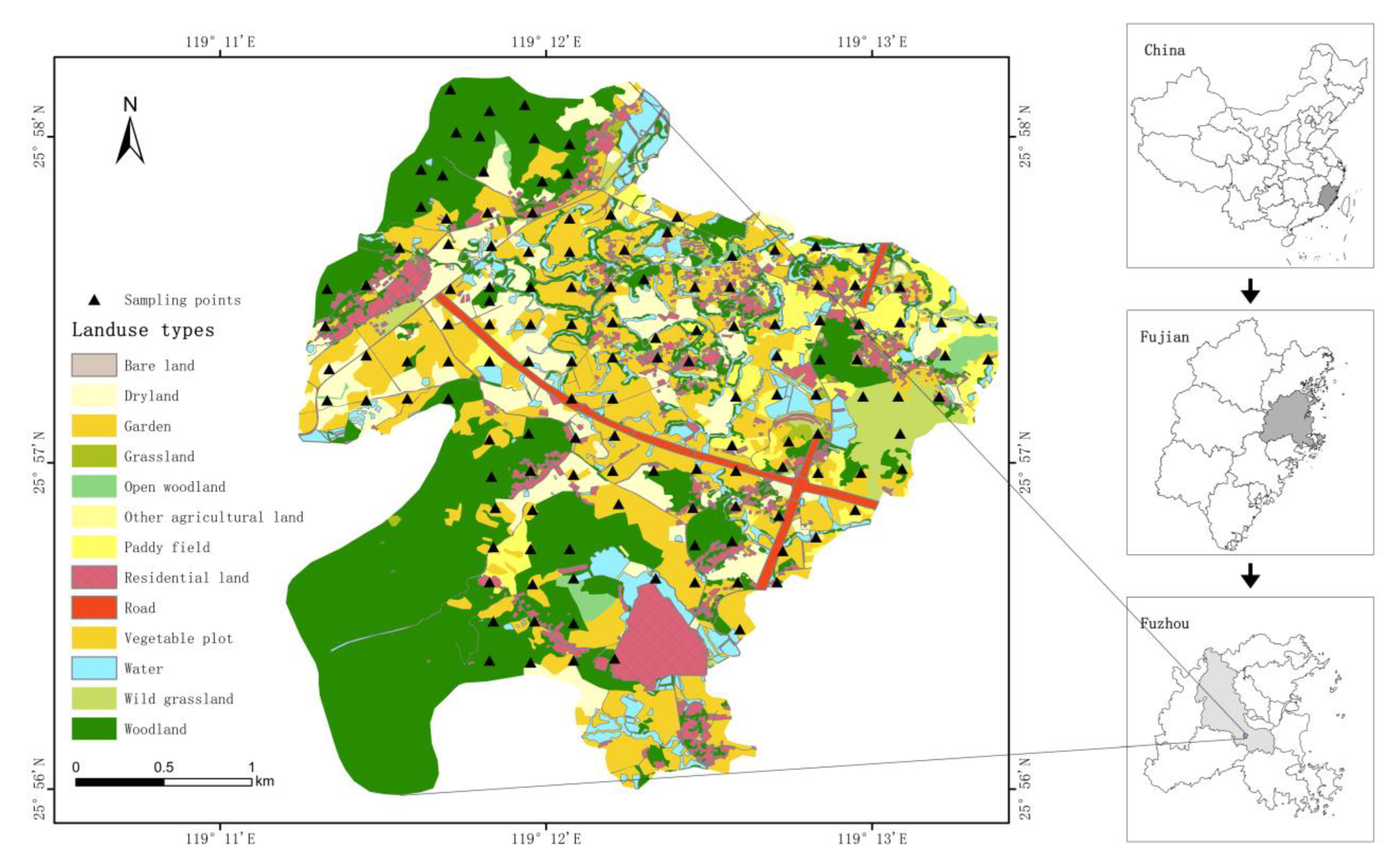
2.1. Study Area

The study area is located in Nanyu, Fuzhou City, Fujian Province (119°11′ E~119°13′ E, 25°55′~25°58′ N) and occupies 9 km2. The average annual temperature is 19.5 °C, and the average annual rainfall is 1340 mm. The area is surrounded by mountains in the north and east, with high terrain, while the central and western parts are flatter and lower, with elevations ranging from 13–451 m. The land use in this area has 13 land types (Figure 1), such as residential land, paddy fields, garden land, forest land, etc. The proportion of different land uses in descending order is: woodland > vegetable plot > dryland > water > residential land > garden > paddy field > wild grassland > road > open woodland > grassland > other agricultural land > bare land. The primary soil type is primarily red soil, the parent material of which is ferralsols or argi-udic ferrosols based on FAO [29] or Chinese Soil Taxonomy [30].

2.2. Soil Sampling and Laboratory Analysis

In 2014, soil samples were collected randomly within a grid size of approximately 200 m∗200 m each, covering the entire study area. A total of 134 surface soil samples (0~20 cm) were collected within five meters of the sample points with multi-point mixed sampling. At the same time, their coordinate locations, elevations, and land use types were recorded by GPS (Figure 1). After removing the residuals with naked eyes, all samples were air-dried and determined in the laboratory at a 1:2.5 soil to solution ratio using a pH detector (PHS-3C, Sheng Ci, Shanghai, China).

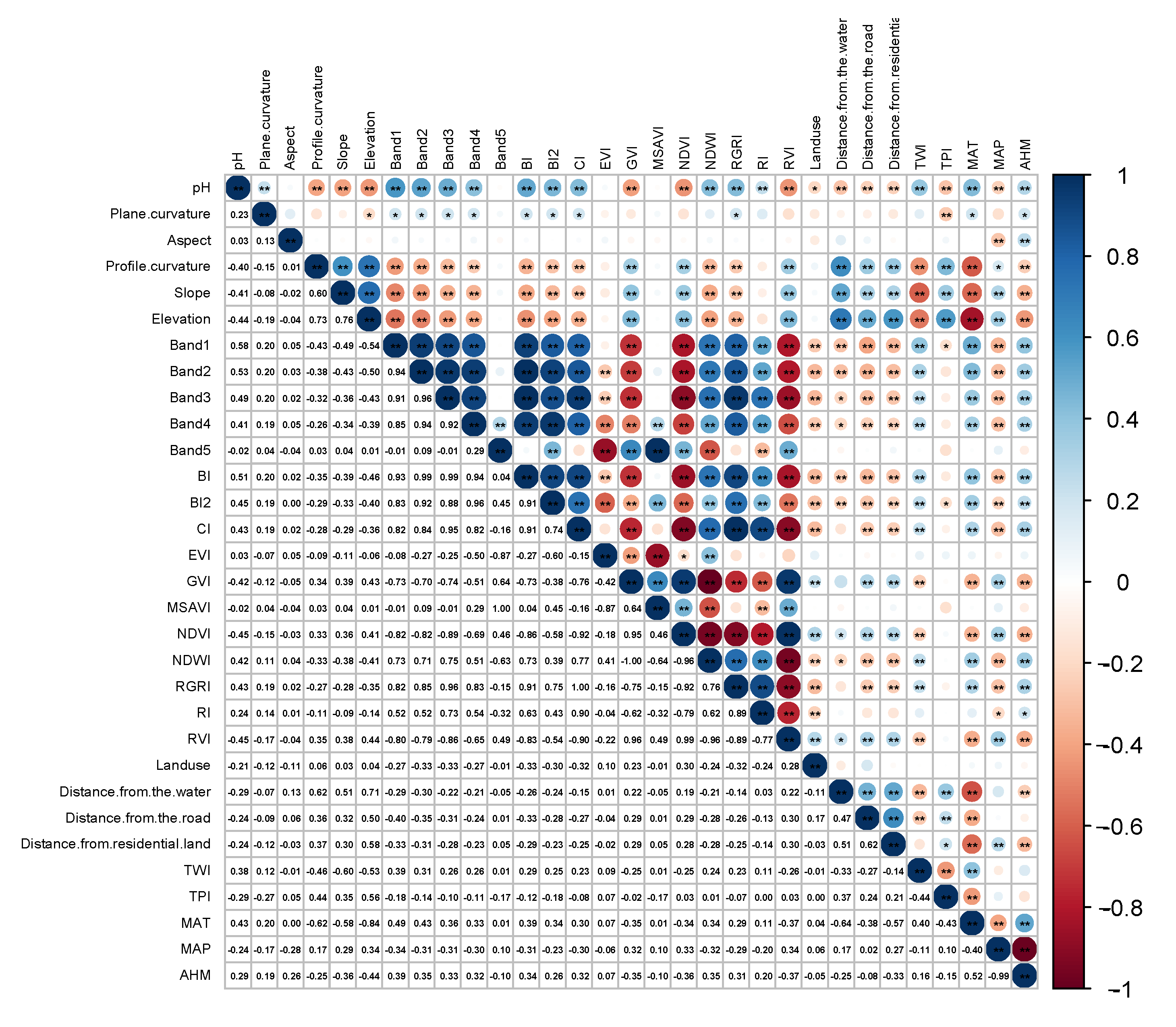
2.3. Environmental Covariates

Thirty environmental variables were selected in this study to predict the soil pH (Table 1).
In this paper, the high-resolution climate model ClimateAP [31] is used to generate three environmental variables in ClimateAP: mean annual temperature (MAT), mean annual precipitation (MAP), and annual humidity and heat index (AHM), based on the latitude, longitude, and altitude of the sampling sites. The spatial resolution of the climate data obtained was 5 m.
Five bands of RapidEye-3A remote sensing imagery [32] were used as the environmental variables for predicting soil pH in this study, with a resolution of 5 m. In this study, 11 vegetation indices were calculated using RapidEye remote sensing imagery (Table 1).
A digital elevation model (DEM) with a resolution of 5 m was obtained from the UAV field data to obtain terrain attribute data, including elevation, slope, aspect, plan curvature, profile curvature, topographic wetness index (TWI), and topographic position index (TPI) [33] (Table 1). The terrain attribute data were all calculated and obtained in ArcGIS 10.2.
The land-use map was obtained using the Second National Land Survey data and visual interpretation. The soil pH was predicted by extracting the distance from the sampling point to the road, distance from the water, and distance from the residential land as environmental variables through ArcGIS 10.2.
After collecting all the variables, the process of this study was divided into three main parts: (i) data preparation and creation of different datasets; (ii) feature selection and model building; and (iii) model performance analysis and spatial distribution mapping.

2.4. Data Pre-Processing

A suitable method to filter valid variables before modeling can reduce information redundancy and optimize the model [35,36]. The support vector machine recursive feature elimination (SVM-RFE) algorithm is used for variable selection and input selection strategy for prediction models, where all the possible inputs are examined based on their influence on the output [37]. The less critical inputs are discarded in every iteration to identify the most suitable set of inputs as predictors [38].
The SVM-RFE calculates the influence of each input through an iterative method. It takes a set of inputs as predictors and an optimal feature subset data as the output to estimate the importance of each piece of information. The inputs showing less influence will be discarded. Finally, this step will finish until the optimum subset of inputs is found.

2.5. Modeling Processes

Here, to predict the soil pH, we used four machine learning models: multiple linear regressions (MLR), random forest (RF), gradient boosting decision tree (GBDT), and extreme gradient boosting (XGBoost). Each model was constructed using 70% of the data as training data, and the remaining 30% of the data was used to evaluate model accuracy.
MLR is a linear regression technique that, unlike simple linear regression analysis, is very useful for studying the linear relationship between a dependent variable and two or more other independent variables [39]. Linear regression in Python 3.8 was used to construct MLR models for soil pH prediction.
RF is a supervised machine learning technique widely used in soil science [40], and it has been indicated that the method is effective in predicting both soil properties [41] and soil classification [42] with high prediction performance. The method is based on decision trees, which generate the results of multiple decision trees for prediction based on randomly selected data to reduce overfitting. The RandomForestRegressor from the sklearn package in Python 3.8 was performed here.
The GBDT model is a combination of the decision tree and boosting algorithm proposed by Friedman [43], which uses gradient, boosting, and decision trees to solve classification problems and perform regression prediction. GBDT is more sensitive to outliers than the random forest and is an integrated tree model that calculates the residuals between actual and predicted values, which can improve performance by reducing the variance of the model [44]. GBDT can be used for classification and regression problems and is one of the best algorithms for fitting the actual distribution [45]. The construction and optimization of the GBDT regression model in this study are proposed using the GradientBoostingRegressor of the sklearn package in Python 3.8.
XGBoost, an algorithm proposed by Chen [46] in 2016, is an integrated machine learning algorithm based on decision trees using gradient boosting as a framework, with high accuracy, scalability, and resistance to overfitting [47]. One of the advantages of XGBoost is that it can handle sparse data and classification and regression tasks. Another advantage of the model is that it can optimize the model to prevent overfitting, and the generalization ability will be more vital. The construction and optimization of the XGBoost regression model in this study are proposed using the XGBRegressor of the sklearn package in Python 3.8.

2.6. Model Evaluation

Different metrics can be used for accuracy evaluation to determine which method is most suitable for soil pH prediction. In this study, three commonly used accuracy evaluation metrics were used to assess the performance of different machine learning models, including the coefficient of determination (R2), root mean square error (RMSE), and mean absolute error (MAE):
R 2 = i = 1 n ( x i y i ¯ ) 2 i = 1 n ( y i y i ¯ ) 2
RMSE = 1 n i = 1 n ( x i y i ) 2
MAE = 1 n i = 1 n | x i y i | y i
where x i is the predicted value of the soil pH, y i is the measured value of the soil pH, and n indicates the number of soil samples. Regarding validation metrics, the closer R2 is to 1, and the closer RMSE and MAE are to 0, the better the model performance, the higher the estimation accuracy, and the smaller the error.

3. Results

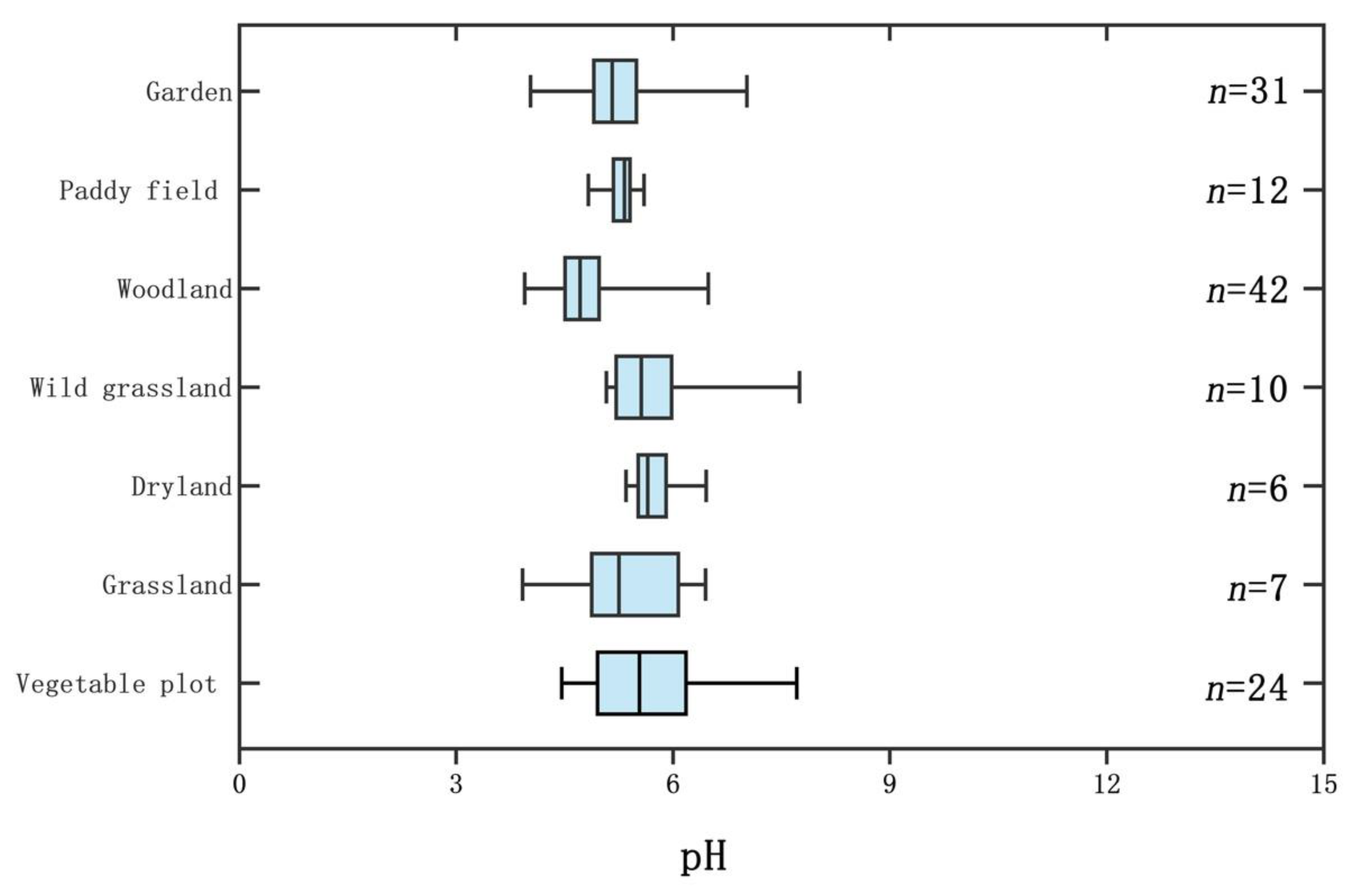
3.1. Descriptive Statistics of Soil pH

Firstly, the soil pH sample data were processed for outliers, and two outliers were removed, leaving 132 sampling points. Secondly, descriptive statistics of the soil pH were determined for the collected sample data (Table 2), and the results showed that the samples of soil pH ranged from 3.95 to 7.75, with a mean value of 5.25 and a coefficient of variation of 14.22%, indicating a moderate variability [48].
According to the soil pH classification criteria [49] (Table 3), it could be found that 58.33% of the sample sites in this study were acidic, 37.12% were strongly acidic, 2.27% were neutral samples, 2.27% were alkaline samples, and there were no strongly alkaline samples.
The soil pH values (Figure 2) varied with land use types, with the mean values showing that wild grassland > dryland > vegetable plot > grassland > paddy field > garden > woodland.

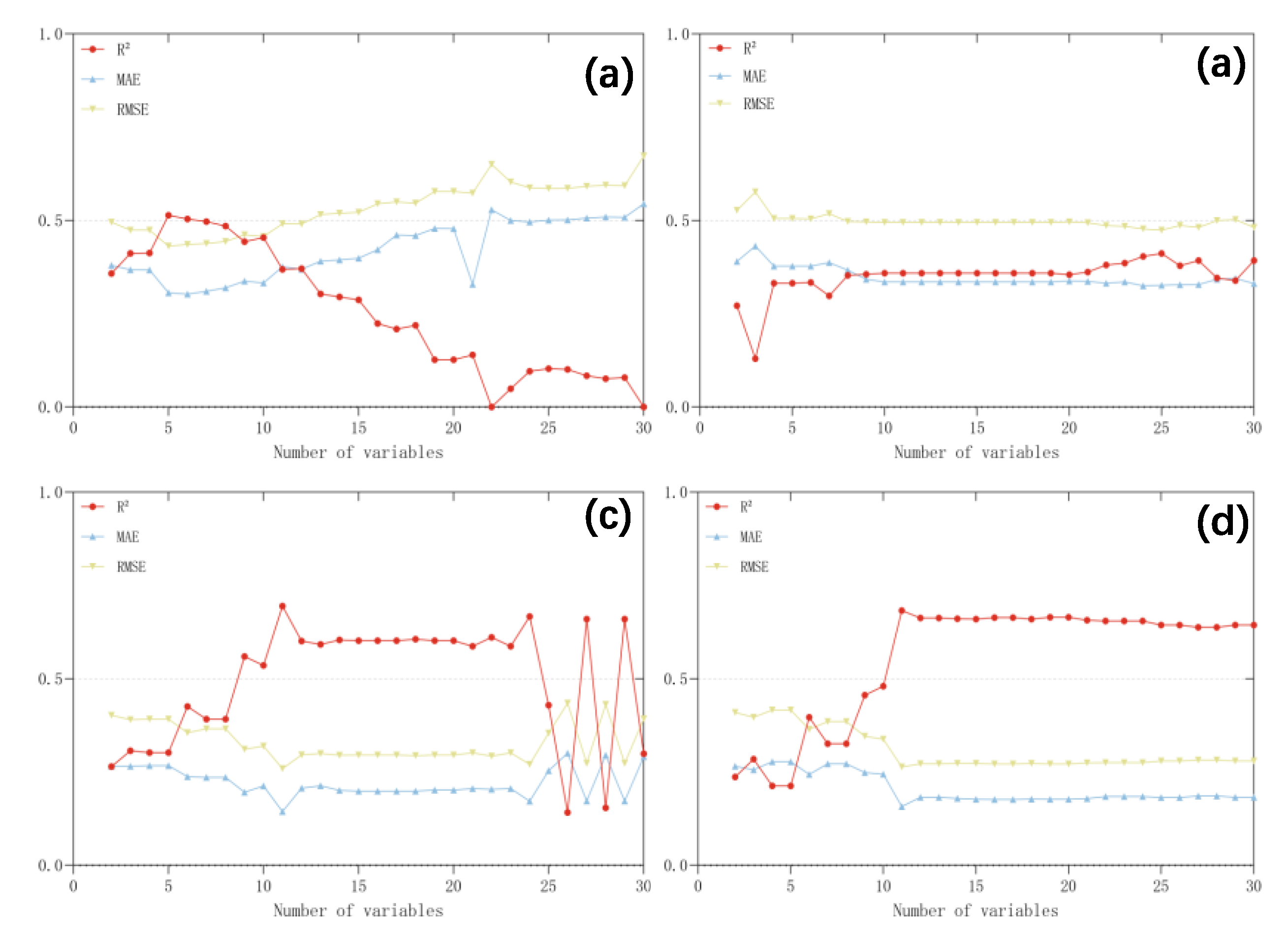
3.2. Feature Selection Procedures

Firstly, a Pearson correlation analysis was carried out between soil pH and the original environmental variables. As can be seen from the heat map (Figure 3), soil pH correlated differently with plane curvature, profile curvature, slope, elevation, Band1, Band2, Band3, Band4, BI, BI2, color index (CI), green vegetation index (GVI), and normalized difference vegetation index (NDVI), and normalized difference water index (NDWI), ratio green-red index (RGRI), redness index (RI), ratio vegetation index (RVI), land use, distance from the water, distance from the road, distance from residential land, topographic wetness index (TWI), topographic position index (TPI), MAT, MAP, and annual humidity-heat index (AHM) were significantly correlated (p < 0.05).
To further investigate the environmental variables for predicting soil pH, the SVM-RFE algorithm was used to select the environmental variables. After several iterations, the features that had a minor influence on the pH prediction results were removed. Then, the remaining features were retrained to obtain a new feature ranking, and the process was iterated again to finally obtain the feature ranking filtered by the SVM-RFE method (Table 4). The results showed that the five most critical environmental variables for the soil pH value included mean annual temperature (MAT), slope, Topographic Wetness Index (TWI), modified soil-adjusted vegetation index (MSAVI), and Band5. The least essential variable was NDVI.
To avoid the influence of multicollinearity between variables on the study results, environmental variables with VIF < 10 were further screened after the SVM-RFE feature selection. Although some of the environmental variables did not correlate significantly with soil pH values, the variables were not necessarily completely independent. The original set of all environmental variables was chosen as a control group for this study and was compared with the set of features selected by the SVM-RFE features.

3.3. Model Performance

According to the importance ranking of SVM-RFE feature selection, four different machine learning models were cyclically modeled with varying environmental variables, and the optimal set of environmental variable features for other models was selected according to R2, MAE, and RMSE. Figure 4 shows that the accuracy of the same model built with different sets of environmental variables changed, and selecting the appropriate set of environmental variables could improve the model prediction accuracy.
The results showed that MAT was the key factor influencing soil pH, indicating that climate significantly affects the prediction of soil pH. Secondly, the TWI and slope, two topographic factors, also greatly influenced the prediction of soil pH. Moreover, MSAVI was another critical factor influencing soil pH. In addition, the results showed that Band5 in the Rapideye image was a good indicator of soil pH. The result was consistent with RAO [50].
Table 5 shows the best set of environment variables for the four machine learning models, illustrating the differences in the best environment variables for the different models. The best set of environment variables for MLR was the top five environment variables obtained by the SVM-RFE algorithm. The best set of environment variables for random forest included twenty-five variables, such as MAT, slope, TWI, and MSAVI. The best environment variables for GBDT model and XGBoost included 11 variables.
After SVM-RFE feature selection for different sets of environmental variables, the accuracy of the other prediction models for pH was assessed by five-fold cross-validation based on R2, MAE, and RMSE to further compare the model accuracy of other machine learning models before and after optimization by the SVM-RFE feature selection algorithm (Table 6). The results indicated that all four machine learning models improved their prediction accuracy substantially after feature selection, especially MLR model, which improved the most in model accuracy (R2 from 0.00 to 0.51). The RF model improved its R2 by 5.64% (from 0.39 to 0.41). The GBDT model improved its R2 by enhancing it by 127.42% (from 0.30 to 0.68). The XGBoost model improved its R2 by 6.06% (from 0.64 to 0.68).
The different machine learning models differed in their ability to predict soil pH in the study area. The XGBoost model was the best predictor before the SVM-RFE selection of variables (R2 = 0.64, MAE = 0.18, RMSE = 0.28). After the SVM-RFE selection of variables, the GBDT model prediction accuracy improved substantially, with R2 increasing to 0.68, MAE decreasing to 0.16, and RMSE decreasing to 0.27. The XGBoost model still performed the best (R2 = 0.68, MAE = 0.16, RMSE = 0.26) compared with the prediction accuracy of Roudier [51] using QRF for soil pH distribution in New Zealand (R2 = 0.65, RMSE = 0.54) and the results of Lu [52] using a Boruta-based support vector regression algorithm for soil pH prediction in Anhui Province (R2 = 0.62, MAE = 0.58, RMSE = 0.73). It can be found that the extreme gradient boosting (XGBoost) prediction model and the gradient boosting decision tree (GBDT) in this study had a higher accuracy than the other two models. However, there is still room for improving the accuracy of the model due to the influence of land use dynamics, different soil parent material types, and complex topography in the study area.
Table 6 shows that the model accuracy of the non-linear models (RF, GBDT, XGBoost) is significantly better than the linear models (MLR) overall. The results indicate a non-linear relationship between the spatial distribution of soil pH and environmental variables, and those non-linear models can better capture and explain changes in soil pH. Hence, such non-linear machine learning models are widely cited in digital soil mapping [53].

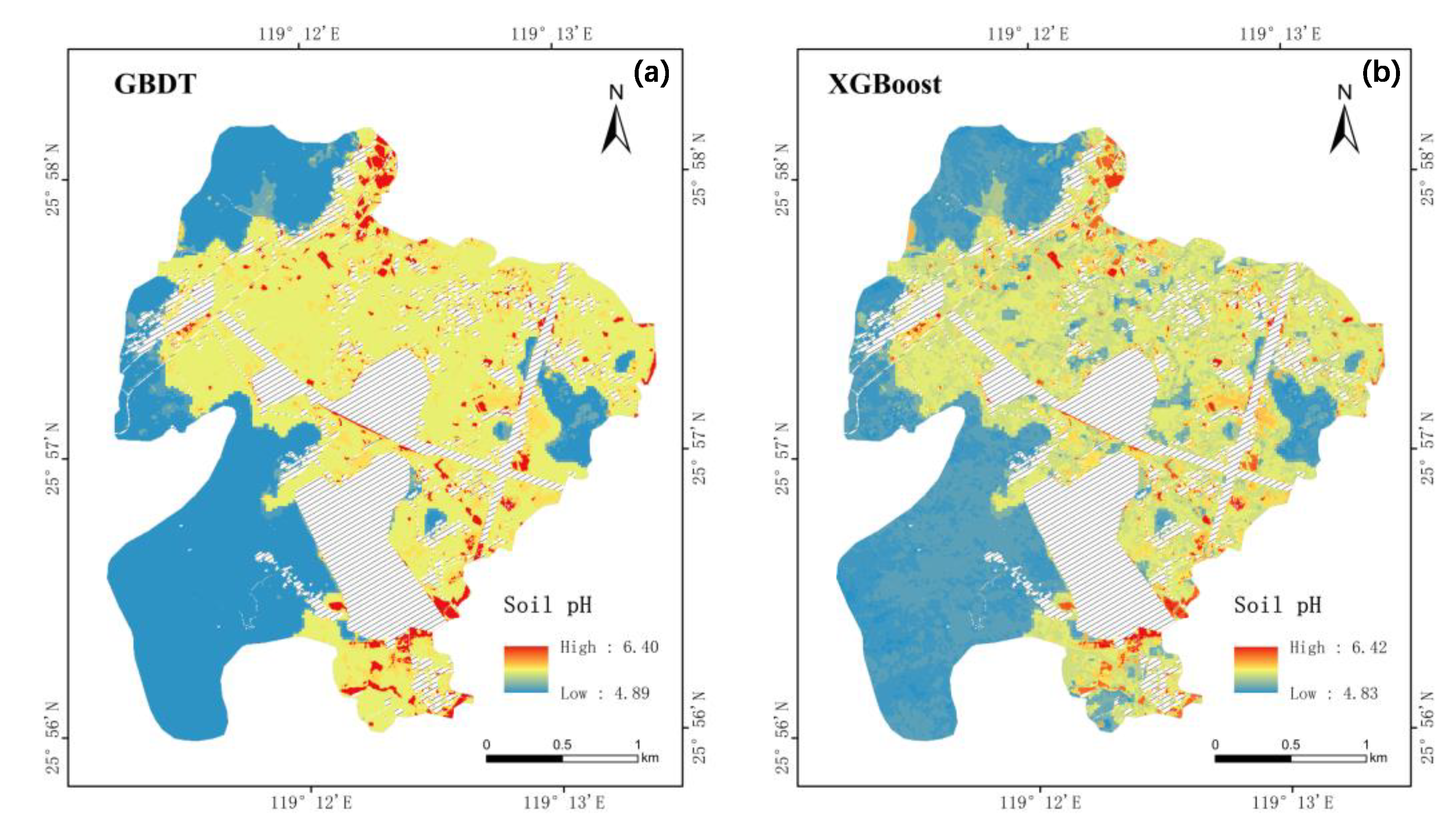
3.4. Spatial Predictive Mapping of Soil pH

Due to the poor accuracy of the MLR and RF soil pH prediction models, only the XGBoost model and the GBDT model based on the SVM-RFE feature selection was constructed to predict the spatial distribution of soil pH in this paper. The results are shown in Figure 5.
Similarities existed between the predictions of the two models (Figure 5), as the study area had mainly acidic and strongly acidic soils. Combined with Figure 5 and the land-use types map of the study area (Figure 1), it can be seen that the areas with high pH values were mainly located in paddy fields and vegetable fields. In contrast, the low-value regions were primarily located in bare land and woodland areas. When the prediction outcomes of the two models were compared, it was found that the XGBoost model had a better high- and low-value predictive capability than the GBDT model.

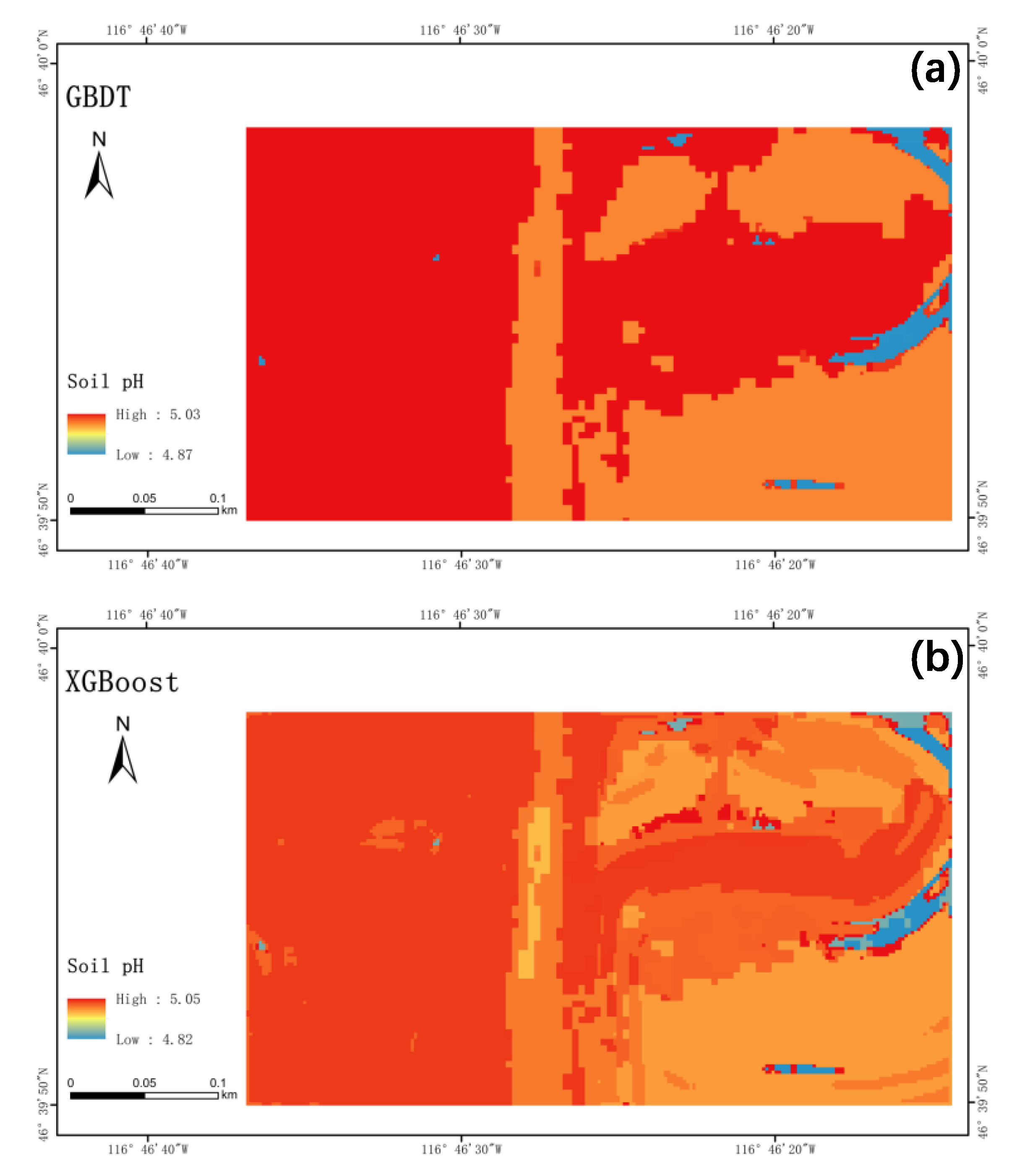
3.5. Assessment of the Generalizability of the Model

To assess the cross-spatial generalizability of the models derived from this study to small- and medium-sized regions, the XGBoost and GBDT models containing 11 environmental variables were applied to soil pH predictions in Pullman, Washington (WA), located in eastern Washington. The Palouse region consists of fertile rolling hills, primarily farmed as rainfed wheat cropping systems with various crop rotations, including canola (Brassica napus), garbanzo beans (Cicer arietinum), and lentils (Lens Cullinaris).
Table 7 shows the prediction accuracy of the two models in this region. The comparison of the two models was consistent with the research results of this paper. The XGBoost model performed better than the GBDT model, and the goodness of fit was above 50%, which was relatively reasonable and accurate. Although the R2 comparison between the two models declined in the soil pH prediction results of the Fuzhou study area, the MAE and RMSE indicators were considerably better than those of the Fuzhou study area. It indicated that the model in this paper had some cross-spatial generality. The prediction accuracy could be improved by selecting a suitable set of environmental variables through RFE-SVM features and machine learning models, which perform better in different regions.
Figure 6 shows the predicted spatial distribution of the region using the XGBoost and GBDT models containing 11 sets of environmental variables. From Figure 6, it can be found that there was spatial variability in the soil pH in the Palouse region, with similar predictions from both models and a consistent trend in spatial distribution, showing an overall acidic soil, in the left half of the region, with low-value areas sporadically distributed, mainly on the right edge. However, XGBoost had better predictive power than GBDT for high and low values, and the predictions were more spatially variable.

4. Discussion

4.1. Subsection Selected Features and Their Implications

Soil pH is an essential factor controlling soil properties. Changes in soil pH are related to climate, land use, nitrogen deposition, and plants [54]. In this study, the selected features of the optimal GBDT model were MAT, slope, TWI, MSAVI, Band5, land use, AHM, TPI, RVI, elevation, and profile curvature.
The plant characters are essential in regulating soil pH [55]. Specifically, plants affect surface roughness, nutrient capture, and ion leaching [56]. In addition, plants regulate soil pH through the uptake of exchangeable cations, alteration of the quality and quantity of apoplastic inputs, and inter-root processes [55]. Consistent with the results of this study, vegetation indices were commonly applied to express the state of vegetation growth and were found to be good predictors of soil pH [21]. In addition, research results confirmed that climate also affected soil pH, with temperature being an important factor in soil pH. Temperature affects soil microbial activity and soil moisture content, causing changes in soil pH [17]. Topographical factors also tend to impact soil pH, with topography allowing for differences in soil and parent material under different light, heat, water, or diving conditions, often leading to spatial variation in the soil pH [24,25]. Similar to the findings of this paper, land use is often closely related to soil pH [22] and rational land use has a positive effect on improving soil structure, strengthening soil resistance, and maintaining and improving soil quality [23].

4.2. Model Comparisons

In this paper, we used the SVM-RFE feature selection algorithm combined with four machine learning models to select the most appropriate set of environmental variables for different models to predict and map the spatial distribution of soil pH in the urban–rural intersection. The results showed significant differences in the predictive power of the other models (Table 6).
Compared with the MLR and RF, XGBoost model and GBDT model performed better, with a higher explained variance and lower error. The XGBoost model was the best predictor before the SVM-RFE selection of variables (R2 = 0.64, MAE = 0.18, RMSE = 0.28). After the SVM-RFE selection of variables, the GBDT model prediction accuracy improved substantially, with R2 increasing to 0.68, MAE decreasing to 0.16, and RMSE decreasing to 0.27. The XGBoost model still performed the best (R2 = 0.68, MAE = 0.16, RMSE = 0.26). In line with the findings of Guo [57] and Ye [58], XGBoost and GBDT model were effective methods for predicting soil property values, reducing the problem of overestimation and underestimation.
Firstly, XGBoost can effectively correct residual errors by generating a new tree based on the previous one [59]. The over-fitting issue with traditional decision trees [60] is resolved by the GBDT model, which applies the gradient descent approach and integrates the decision tree method with the bagging and boosting algorithm [61]. Secondly, compared to RF models, where the tree is independent in the RF model, XGBoost and GDBT are two more flexible algorithms responsible for their better performance. Thirdly, XGBoost improves the GBDT model at the algorithmic level compared with GBDT. The prediction accuracy and efficiency of XGBoost are higher than that of the GBDT model [58]. Finally, XGBoost and GBDT, as two non-linear models, can better capture and explain changes in soil pH than a non-linear model such as multiple linear regression [53].

4.3. Limitations and Future Research

Firstly, in this study, soil pH, as a regionalized variable, is dynamically influenced by a compound of multiple environmental variables [3,4,5,6]. Therefore, exploring the influence of more environmental variables when mapping the spatial distribution of soil pH is necessary. In future studies, more characteristic variables that have an essential impact on soil pH can be added to the model, including natural factors such as soil parent material and soil type [62], which strongly influence soil pH, as well as anthropogenic factors such as industrial pollution from urbanization and agricultural fertilization activities [63,64,65]. Secondly, this paper only uses the SVM-RFE feature selection algorithm in combination with four machine learning models. It does not reflect whether the SVM-RFE feature selection algorithm is the most appropriate feature selection method, while many feature selection methods exist. According to past research [66,67], it can be found that feature selection methods can effectively improve soil attribute prediction accuracy. Different feature selection methods have different effects on improving model accuracy. In subsequent research, the various feature selection methods can be compared to demonstrate the superiority of the SVM-RFE feature selection method.

5. Conclusions

Combined SVM-RFE feature selection methods with four machine learning models to predict and map the spatial distribution of soil pH were conducted using environmental variables, including topographic data, remote sensing images, soil measurement data, and climate data. We found that: (1) the five most important environmental variables affecting soil pH were obtained using the SVM-RFE feature selection method; they were MAT, slope, TWI, MSAVI, and Band5; (2) the SVM-RFE feature selection methods combined with different machine learning models can improve model accuracy; (3) different machine learning models differed in their ability to predict soil pH, both before and after feature selection, and XGBoost method is the best. This paper validates the impact of the SVM-RFE feature selection method on soil pH prediction, provides a new fast and highly accurate mapping method for predicting soil pH, and constructs a reliable, small area-scale soil pH prediction model.

Author Contributions

Conceptualization, K.W. and S.J.; methodology, J.G. and S.J.; software, J.G.; validation, J.G. and S.J.; formal analysis, J.G.; investigation, K.W.; resources, K.W.; data curation, J.G.; writing—original draft preparation, J.G.; writing—review and editing, K.W. and S.J.; visualization, J.G.; supervision, K.W. and S.J.; project administration, K.W. and S.J.; funding acquisition, K.W. and S.J. All authors have read and agreed to the published version of the manuscript.

Funding

This research was funded by the Technology Innovation Center for Monitoring and Restoration Engineering of the Ecological Fragile Zone in Southeast China, MNR, grant number KY-090000-04-2021-009; the Natural Science Foundation of Fujian Province, China (Grant No. 2022J011140); and the central government guides local projects (Grant NO 2020L3024).

Data Availability Statement

Not applicable.

Conflicts of Interest

The authors declare no conflict of interest.

References

  1. Wang, Z.; Shen, F.; Shen, D.; Jiang, Y.; Xiao, R. Immobilization of Cu2+ and Cd2+ by earthworm manure derived biochar in acidic circumstance. J. Environ. Sci. 2017, 53, 293–300. [Google Scholar] [CrossRef] [PubMed]
  2. Neina, D. The Role of Soil pH in Plant Nutrition and Soil Remediation. Appl. Environ. Soil Sci. 2019, 2019, 5794869. [Google Scholar] [CrossRef] [Green Version]
  3. Xiang, J.; Song, C.; Shi, Y.; Dong, Q.; Yang, Z. Spatial Variation Characteristics and Influencing Factors of Soil pH in the Lu′an Area of Anhui Province. Chin. J. Soil Sci. 2021, 52, 34–41. [Google Scholar]
  4. Mao, W.; Li, W.; Gao, H.; Chen, X.; Jiang, Y.; Hang, T.; Gong, X.; Chen, M.; Zhang, Y. pH variation and the driving factors of farmlands in Yangzhou for 30 years. J. Plant Nutr. Fertitizer 2017, 23, 883–893. [Google Scholar]
  5. Johnston, A.E.; Goulding, K.W.T.; Poulton, P.R. Soil acidification during more than 100 years under permanent grassland and woodland at rothamsted. Soil Use Manag. 1986, 2, 3–10. [Google Scholar] [CrossRef]
  6. Kopittke, G.R.; Tietema, A.; Verstraten, J.M. Soil acidification occurs under ambient conditions but is retarded by repeated drought: Results of a field-scale climate manipulation experiment. Sci. Total Environ. 2012, 439, 332–342. [Google Scholar] [CrossRef]
  7. Sun, F.; Lei, Q.; Liu, Y.; Li, H.; Wang, Q. The Progress and Prospect of Digital Soil Mapping Research. J. Soil Sci. 2011, 42, 1502–1507. [Google Scholar]
  8. Zeng, C.; Zhu, A.X.; Liu, F.; Yang, L.; Rossiter, D.G.; Liu, J.; Wang, D. The impact of rainfall magnitude on the performance of digital soil mapping over low-relief areas using a land surface dynamic feedback method. Ecol. Indic. 2017, 72, 297–309. [Google Scholar] [CrossRef]
  9. Malone, B.P.; Mcbratney, A.B.; Minasny, B.; Laslett, G.M. Mapping continuous depth functions of soil carbon storage and available water capacity. Geoderma 2009, 154, 138–152. [Google Scholar] [CrossRef]
  10. Yang, R.-M.; Zhang, G.-L.; Liu, F.; Lu, Y.-Y.; Yang, F.; Yang, F.; Yang, M.; Zhao, Y.-G.; Li, D.-C. Comparison of boosted regression tree and random forest models for mapping topsoil organic carbon concentration in an alpine ecosystem. Ecol. Indic. Integr. Monit. Assess. Manag. 2016, 60, 870–878. [Google Scholar] [CrossRef]
  11. Cai, H.; Peng, J.; Liu, W.; Luo, D.; Wang, Y.; Bai, J.; Bai, Z. Inversion and Mapping of Soil pH Valve Based on In-situ Hyperspectral Data in Cotton field. Bull. Soil Water Conserv. 2021, 41, 189–195. [Google Scholar]
  12. Dharumarajan, S.; Hegde, R.; Singh, S.K. Spatial prediction of major soil properties using Random Forest techniques A case study in semi-arid tropics of South India. Geoderma Reg. 2017, 10, 154–162. [Google Scholar] [CrossRef]
  13. Pahlavan-Rad, M.R.; Akbarimoghaddam, A. Spatial variability of soil texture fractions and pH in a flood plain (case study from eastern Iran). Catena 2018, 160, 275–281. [Google Scholar] [CrossRef]
  14. Tumsavas, Z. Possibility of determining soil pH using visible and near-infrared (Vis-NIR) spectrophotometry. J. Environ. Biol. 2017, 38, 1095–1100. [Google Scholar] [CrossRef]
  15. Wang, K. Application of geographically weighted regression on the spatial prediction of soil pH. J. Hunan Agric. Univ. 2013, 39, 73–79. [Google Scholar] [CrossRef]
  16. Chen, S.; Liang, Z.; Webster, R.; Zhang, G.; Zhou, Y.; Teng, H.; Hu, B.; Arrouays, D.; Shi, Z. A high-resolution map of soil pH in China made by hybrid modelling of sparse soil data and environmental covariates and its implications for pollution. Sci. Total Environ. 2019, 655, 273–283. [Google Scholar] [CrossRef]
  17. Yang, L.; Lin, J.; Molder, E.; Gao, R.; Yu, H.; Lin, Y.; Wang, D.; Li, J. Effects of Climate Types and Slope Sections on the pH of Soil in the Unstable Slope with High-Frequency Debris Flow in Jiangjiagou Watershed of Yunnan Province. Res. Soil Water Conserv. 2022, 29, 105–112. [Google Scholar]
  18. Ma, B.; Wu, F.; Li, Z.; Wang, J. Interaction of Crop Cover and Slope Gradient on Runoff and Sediment Yield. J. Soil Water Conserv. 2013, 27, 33–38. [Google Scholar]
  19. Jin, P.; Li, P.; Wang, Q.; Pu, Z. Developing and applying novel spectral feature parameters for classifying soil salt types in arid land. Ecol. Indic. 2015, 54, 116–123. [Google Scholar] [CrossRef]
  20. Bai, L.; Wang, C.; Zang, S.; Zhang, Y.; Hao, Q.; Wu, Y. Remote Sensing of Soil Alkalinity and Salinity in the Wuyu′er-Shuangyang River Basin, Northeast China. Remote Sens. 2016, 8, 163. [Google Scholar] [CrossRef] [Green Version]
  21. Reuter, H.I.; Nelson, A. Chapter 11 Geomorphometry in ESRI Packages. Dev. Soil Sci. 2009, 33, 269–291. [Google Scholar]
  22. Zhou, J.Y.; Zhang, L.M.; Yang, W.H.; Zhou, B.Q.; Xing, S.H. Dynamic and its driving factors of soil potential acid in croplands of Fujian Province, China. Ying Yong Sheng Tai Xue Bao J. Appl. Ecol. 2019, 30, 913–922. [Google Scholar]
  23. Fu, B.J.; Chen, L.D.; Ma, K.M.; Zhou, H.F.; Wang, J. The relationships between land use and soil conditions in the hilly area of the loess plateau in northern Shaanxi, China. Catena 2000, 39, 69–78. [Google Scholar] [CrossRef]
  24. Jolokhava, T.; Abdaladze, O.; Gadilia, S.; Kikvidze, Z. Variable soil pH can drive changes in slope aspect preference of plants in alpine desert of the Central Great Caucasus (Kazbegi district, Georgia). Acta Oecologica-Int. J. Ecol. 2020, 105, 103582. [Google Scholar] [CrossRef]
  25. Baltensweiler, A.; Heuvelink, G.B.M.; Hanewinkel, M.; Walthert, L. Microtopography shapes soil pH in flysch regions across Switzerland. Geoderma 2020, 380, 114663. [Google Scholar] [CrossRef]
  26. Wang, S.-H.; Lu, H.-L.; Zhao, M.-S.; Zhou, L.-M. Assessing soil pH in Anhui Province based on different features mining methods combined with generalized boosted regression models. Ying Yong Sheng Tai Xue Bao J. Appl. Ecol. 2020, 31, 3509–3517. [Google Scholar]
  27. Zhao, J.; Zhang, C.; Min, L.; Li, N.; Wang, Y. Retrieval for soil moisture in farmland using multi-source remote sensing data and feature selection with GA-BP neural network. Trans. Chin. Soc. Agric. Eng. 2021, 37, 112–120. [Google Scholar]
  28. Zeraatpisheh, M.; Garosi, Y.; Owliaie, H.; Ayoubi, S.; Xu, M. Improving the spatial prediction of soil organic carbon using environmental covariates selection: A comparison of a group of environmental covariates. Catena 2022, 208, 105723. [Google Scholar] [CrossRef]
  29. International Union of Soil Sciences Working Group. World Reference Base for Soil Resources 2014: International Soil Classification System for Naming Soils and Creating Legends for Soil Maps; World Soil Resources Reports 106; FAO: Rome, Italy, 2014; Volume 106. [Google Scholar]
  30. Chen, Z.; Gong, Z.; Zhang, G.; Zhao, W. Correlation of soil taxa between chinese soil genetic classification and chinese soil taxonomy on various scales. Soils 2004, 36, 584–595. [Google Scholar]
  31. Wang, T.; Wang, G.; Innes, J.; Nitschke, C.; Kang, H. Climatic niche models and their consensus projections for future climates for four major forest tree species in the Asia-Pacific region. For. Ecol. Manag. 2016, 360, 357–366. [Google Scholar] [CrossRef]
  32. Thu Thuy, N.; Tien Dat, P.; Chi Trung, N.; Delfos, J.; Archibald, R.; Kinh Bac, D.; Ngoc Bich, H.; Guo, W.; Huu Hao, N. A novel intelligence approach based active and ensemble learning for agricultural soil organic carbon prediction using multispectral and SAR data fusion. Sci. Total Environ. 2022, 804, 150187. [Google Scholar]
  33. Odhiambo, B.O.; Kenduiywo, B.K.; Were, K. Spatial prediction and mapping of soil pH across a tropical afro-montane landscape. Appl. Geogr. 2020, 114, 102129. [Google Scholar] [CrossRef]
  34. Mathieu, R.; Pouget, M.; Cervelle, B.; Escadafal, R. Relationships between satellite-based radiometric indices simulated using laboratory reflectance data and typic soil color of an arid environment. Remote Sens. Environ. 1998, 66, 17–28. [Google Scholar] [CrossRef]
  35. Taghizadeh-Mehrjardi, R.; Schmidt, K.; Amirian-Chakan, A.; Rentschler, T.; Zeraatpisheh, M.; Sarmadian, F.; Valavi, R.; Davatgar, N.; Behrens, T.; Scholten, T. Improving the Spatial Prediction of Soil Organic Carbon Content in Two Contrasting Climatic Regions by Stacking Machine Learning Models and Rescanning Covariate Space. Remote Sens. 2020, 12, 1095. [Google Scholar] [CrossRef] [Green Version]
  36. Tajik, S.; Ayoubi, S.; Zeraatpisheh, M. Digital mapping of soil organic carbon using ensemble learning model in Mollisols of Hyrcanian forests, northern Iran. Geoderma Reg. 2020, 20, e00256. [Google Scholar] [CrossRef]
  37. Tao, H.; Al-Bedyry, N.K.; Khedher, K.M.; Shahid, S.; Yaseen, Z.M. River water level prediction in coastal catchment using hybridized relevance vector machine model with improved grasshopper optimization. J. Hydrol. 2021, 598, 126477. [Google Scholar] [CrossRef]
  38. Huang, X.; Zhang, L.; Wang, B.; Li, F.; Zhang, Z. Feature clustering based support vector machine recursive feature elimination for gene selection. Appl. Intell. 2018, 48, 594–607. [Google Scholar] [CrossRef]
  39. Williams, C.G.; Ojuri, O.O. Predictive modelling of soils’ hydraulic conductivity using artificial neural network and multiple linear regression. SN Appl. Sci. 2021, 3, 152. [Google Scholar] [CrossRef]
  40. Breiman, L. Random forests, machine learning 45. J. Clin. Microbiol. 2001, 2, 199–228. [Google Scholar]
  41. Pham, T.D.; Yokoya, N.; Nguyen, T.T.T.; Le, N.N.; Ha, N.T.; Xia, J.; Takeuchi, W.; Pham, T.D. Improvement of Mangrove Soil Carbon Stocks Estimation in North Vietnam Using Sentinel-2 Data and Machine Learning Approach. Giscience Remote Sens. 2021, 58, 68–87. [Google Scholar] [CrossRef]
  42. Teng, H.; Rossel, R.A.V.; Shi, Z.; Behrens, T. Updating a national soil classification with spectroscopic predictions and digital soil mapping. Catena 2018, 164, 125–134. [Google Scholar] [CrossRef]
  43. Friedman, J.H. Greedy function approximation: A gradient boosting machine. Ann. Stat. 2001, 29, 1189–1232. [Google Scholar] [CrossRef]
  44. Jin, X.; Zhu, X.; Li, S.; Wang, W.; Qi, H. Predicting Soil Available Phosphorus by Hyperspectral Regression Method Based on Gradient Boosting Decision Tree. Laser Optoelectron. Prog. 2019, 56, 141–150. [Google Scholar]
  45. Song, Y.; Niu, R.; Xu, S.; Ye, R.; Peng, L.; Guo, T.; Li, S.; Chen, T. Landslide Susceptibility Mapping Based on Weighted Gradient Boosting Decision Tree in Wanzhou Section of the Three Gorges Reservoir Area (China). ISPRS Int. J. Geo-Inf. 2019, 8, 4. [Google Scholar] [CrossRef]
  46. Chen, T.; Guestrin, C.; Assoc Comp, M. XGBoost: A Scalable Tree Boosting System. In Proceedings of the 22nd ACM SIGKDD International Conference on Knowledge Discovery and Data Mining (KDD), San Francisco, CA, USA, 13–17 August 2016; pp. 785–794. [Google Scholar]
  47. Jia, Y.; Jin, S.; Savi, P.; Gao, Y.; Tang, J.; Chen, Y.; Li, W. GNSS-R Soil Moisture Retrieval Based on a XGboost Machine Learning Aided Method: Performance and Validation. Remote Sens. 2019, 11, 1655. [Google Scholar] [CrossRef] [Green Version]
  48. Nam Thang, H.; Manley-Harris, M.; Tien Dat, P.; Hawes, I. The use of radar and optical satellite imagery combined with advanced machine learning and metaheuristic optimization techniques to detect and quantify above ground biomass of intertidal seagrass in a New Zealand estuary. Int. J. Remote Sens. 2021, 42, 4716–4742. [Google Scholar]
  49. Nielsen, D.R.; Bouma, J. Soil Spatial Variability: Proceedings of a Workshop of the ISSS and the SSSA, Las Vegas, USA/Pdc296; Center Agricultural Pub and Document: Wageningen, The Netherlands, 1985. [Google Scholar]
  50. Rao, B.R.M.; Sharma, R.C.; Ravi Sankar, T.; Das, S.N.; Dwivedi, R.S.; Thammappa, S.S.; Venkataratnam, L. Spectral behaviour of salt-affected soils. Int. J. Remote Sens. 1995, 16, 2125–2136. [Google Scholar] [CrossRef]
  51. Roudier, P.; Burge, O.R.; Richardson, S.J.; McCarthy, J.K.; Grealish, G.J.; Ausseil, A.-G. National Scale 3D Mapping of Soil pH Using a Data Augmentation Approach. Remote Sens. 2020, 12, 2872. [Google Scholar] [CrossRef]
  52. Lu, H.; Zhao, M.; Liu, B.; Zhang, P.; Lu, L. Predictive Mapping of Soil pH in Anhui Province Based on Boruta-Support Vector Regression. Geogr. Geo-Inf. Sci. 2019, 35, 66–72. [Google Scholar]
  53. Khaledian, Y.; Miller, B.A. Selecting appropriate machine learning methods for digital soil mapping. Appl. Math. Model. 2020, 81, 401–418. [Google Scholar] [CrossRef]
  54. Hong, S.; Gan, P.; Chen, A. Environmental controls on soil pH in planted forest and its response to nitrogen deposition. Environ. Res. 2019, 172, 159–165. [Google Scholar] [CrossRef] [PubMed]
  55. Binkley, D.; Richter, D.D. Nutrient Cycles and H+ Budgets of Forest Ecosystems. Adv. Ecol. Res. 1987, 16, 1–51. [Google Scholar]
  56. Hogberg, P.; Fan, H.B.; Quist, M.; Binkley, D.; Tamm, C.O. Tree growth and soil acidification in response to 30 years of experimental nitrogen loading on boreal forest. Glob. Chang. Biol. 2006, 12, 489–499. [Google Scholar] [CrossRef]
  57. Guo, J.; Zhao, X.; Guo, X.; Zhu, Q.; Luo, J.; Xu, Z.; Zhong, L.; Ye, Y. Inversion of soil properties in rare earth mining areas (southern Jiangxi, China) based on visible-near-infrared spectroscopy. J. Soils Sediments 2022, 22, 2406–2421. [Google Scholar] [CrossRef]
  58. Ye, Z.; Sheng, Z.; Liu, X.; Ma, Y.; Wang, R.; Ding, S.; Liu, M.; Li, Z.; Wang, Q. Using Machine Learning Algorithms Based on GF-6 and Google Earth Engine to Predict and Map the Spatial Distribution of Soil Organic Matter Content. Sustainability 2021, 13, 14055. [Google Scholar] [CrossRef]
  59. Li, Y.; Li, M.; Li, C.; Liu, Z. Forest aboveground biomass estimation using Landsat 8 and Sentinel-1A data with machine learning algorithms. Sci. Rep. 2020, 10, 9952. [Google Scholar] [CrossRef]
  60. Brown, I.; Mues, C. An experimental comparison of classification algorithms for imbalanced credit scoring data sets. Expert Syst. Appl. 2012, 39, 3446–3453. [Google Scholar] [CrossRef]
  61. Rong, G.; Alu, S.; Li, K.; Su, Y.; Zhang, J.; Zhang, Y.; Li, T. Rainfall Induced Landslide Susceptibility Mapping Based on Bayesian Optimized Random Forest and Gradient Boosting Decision Tree Models-A Case Study of Shuicheng County, China. Water 2020, 12, 3066. [Google Scholar] [CrossRef]
  62. Zhang, W.; Li, Q.; Wang, C.; Yuan, D.; Lou, Y.; Zhang, X.; Jia, L. Spatail variability of soil ph and its influence factors at a county scale in hilly area of mid-sichuan basin a case study from renshou in sichuan. Resour. Environ. Yangtze Basin 2015, 24, 1192–1199. [Google Scholar]
  63. Xie, E.; Zhao, Y.; Li, H.; Shi, X.; Lu, F.; Zhang, X.; Peng, Y. Spatio-temporal changes of cropland soil pH in a rapidly industrializing region in the Yangtze River Delta of China, 1980–2015. Agric. Ecosyst. Environ. 2019, 272, 95–104. [Google Scholar] [CrossRef]
  64. Zeng, M.; de Vries, W.; Bonten, L.T.C.; Zhu, Q.; Hao, T.; Liu, X.; Xu, M.; Shi, X.; Zhang, F.; Shen, J. Model-Based Analysis of the Long-Term Effects of Fertilization Management on Cropland Soil Acidification. Environ. Sci. Technol. 2017, 51, 3843–3851. [Google Scholar] [CrossRef] [PubMed]
  65. Zhang, Y.; de Vries, W.; Thomas, B.W.; Hao, X.; Shi, X. Impacts of long-term nitrogen fertilization on acid buffering rates and mechanisms of a slightly calcareous clay soil. Geoderma 2017, 305, 92–99. [Google Scholar] [CrossRef]
  66. Shekofteh, H.; Ramazani, F.; Shirani, H. Optimal feature selection for predicting soil CEC: Comparing the hybrid of ant colony organization algorithm and adaptive network-based fuzzy system with multiple linear regression. Geoderma 2017, 298, 27–34. [Google Scholar] [CrossRef]
  67. Meng, X.; Bao, Y.; Ye, Q.; Liu, H.; Zhang, X.; Tang, H.; Zhang, X. Soil Organic Matter Prediction Model with Satellite Hyperspectral Image Based on Optimized Denoising Method. Remote Sens. 2021, 13, 2273. [Google Scholar] [CrossRef]
Figure 1. Location of the study area.
Agronomy 12 02742 g001
Figure 2. Box plot of soil pH under different land-use practices in the study area.
Agronomy 12 02742 g002
Figure 3. Heat map of the correlation between soil pH and environmental variables (the top right-hand corner is a heat map of the correlation with added significance markers and the bottom left-hand corner is the correlation coefficient r value.).
Agronomy 12 02742 g003
Figure 4. Model performance of different sets of environmental variables after SVM-RFE feature selection. (a) MLR: multiple linear regressions; (b) RF: random forest; (c) GBDT: gradient boosting decision tree; (d) XGBoost: extreme gradient boosting.
Agronomy 12 02742 g004
Figure 5. Map of the XGBoost and GBDT models for predicting soil pH based on SVM-RFE feature selection, excluding building sites. (a) GBDT: gradient boosting decision tree; (b) XGBoost: extreme gradient boosting.
Agronomy 12 02742 g005
Figure 6. Maps for predicting soil pH in the Palouse region based on SVM-RFE feature selection with XGBoost and GBDT models. (a) GBDT: gradient boosting decision tree; (b) XGBoost: extreme gradient boosting.
Agronomy 12 02742 g006
Table 1. Environmental variables used in this study.
DataSource
Climate
Mean annual temperature (MAT)ClimateAP
Mean annual precipitation (MAP)ClimateAP
Annual humidity-heat index (AHM)ClimateAP
Remote sensing image
Band1 (Blue) RapidEye-3A (440–510 nm)
Band2 (Green) RapidEye-3A (520–590 nm)
Band3 (Red) RapidEye-3A (630–685 nm)
Band4 (Red edge) RapidEye-3A (690–730 nm)
Band5 (NIR) RapidEye-3A (760–850 nm)
Vegetation Index
NDVI N I R R e d N I R + R e d
RVI N I R R e d
MSAVI 2 × N I R + 1 ( 2 × N I R + 1 ) 2 8 × ( N I R R e d ) 2
EVI 2.5 × ( N I R R e d ) N I R + 6 × R e d 7.5 × B l u e + 1
RGRI R e d G r e e n
GVI N I R G r e e n
BI [32] ( R e d × R e d ) + ( G r e e n × G r e e n ) 2
BI2 [32] ( R e d × R e d ) + ( G r e e n × G r e e n ) + ( N I R × N I R ) 2
RI [34] R e d × R e d G r e e n × G r e e n × G r e e n
CI [34] R e d G r e e n R e d + G r e e n
NDWI G r e e n N I R G r e e n + N I R
DEM derivatives
Elevation
SlopeThe degree of steepness of a surface element.
AspectThe degree to which the ground tilts.
Plane curvatureThe surface shape is viewed in a horizontal plane that has sliced through the surface at the target point.
Profile curvatureThe shape of the surface in the immediate neighborhood of the sample point was contained within the vertical plane.
TWITopographic Wetness Index.
TPITopographic position index.
Human factors
Land-use map
Distance from the road
Distance from the water
Distance from residential land
Note: NDVI: normalized difference vegetation index; RVI: ratio vegetation index; MSAVI: modified soil-adjusted vegetation index; EVI: enhanced vegetation index; RGRI: ratio green-red index; GVI:green vegetation index; BI: brightness index; BI2: brightness index 2; RI: redness index; CI: color index; NDWI: normalized difference water index.
Table 2. Descriptive statistics of soil pH.
ParameterMinMaxMeanSDCV
pH3.92 7.75 5.25 0.75 14.22%
Table 3. Distribution of acidity and alkalinity at sampling sites.
Strong Acid
(<5.0)
Acid
(5.0~<6.5)
Neutral
(6.5~<7.5)
Alkaline
(7.5~<8.5)
Strong Alkaline
(>8.5)
Frequency of sample point distribution37.12%58.33%2.27%2.27%0.00%
Table 4. The results of the support vector machine recursive feature elimination (SVM-RFE) feature selection.
Feature
Name
Feature RankingFeature
Name
Feature RankingFeature
Name
Feature Ranking
MAT1Profile curvature11Band121
Slope2BI212NDWI22
TWI3BI.13RGRI23
MSAVI 4MAP14RI24
Band55Band315Distance from the water25
Land use6Band216CI26
AHM7Band4 17Distance from the road27
TPI8Plane curvature 18EVI28
RVI 9GVI19Distance from residential land29
Elevation10Aspect 20NDVI30
MAT: mean annual temperature; MAP: mean annual precipitation; AHM: annual humidity-heat index; TWI: Topographic Wetness Index; TPI: topographic position index.
Table 5. The most suitable set of environment variables for different machine learning models.
ModelsThe Optimal Set of Environment VariablesNumber of Variables
MLRMAT, slope, TWI, MSAVI, Band5.5
RFMAT, slope, TWI, MSAVI, Band5, land use, AHM, TPI, RVI, elevation, profile curvature, BI2, BI, MAP, Band3, Band2, Band4, plane curvature, GVI, aspect, NDWI, RGRI, RI, distance from the water.25
GBDTMAT, slope, TWI, MSAVI, Band5, land use, AHM, TPI, RVI, elevation, profile curvature.11
XGBoostMAT, slope, TWI, MSAVI, Band5, land use, AHM, TPI, RVI, elevation, profile curvature.11
MLR: multiple linear regressions; RF: random forest; GBDT: gradient boosting decision tree; XGBoost: extreme gradient boosting; MAT: mean annual temperature; MAP: mean annual precipitation; AHM: annual humidity-heat index; TWI: Topographic Wetness Index; TPI: topographic position index.
Table 6. Comparing accuracy before and after feature selection for different machine learning models. Bold rows are shown as the most accurate results.
ModelsData Sets with Different Characteristic VariablesR2MAERMSE
MLRRaw feature variable dataset0.000.550.67
SVM-RFE feature selection after feature variable dataset0.510.310.43
RFRaw feature variable dataset0.390.330.48
SVM-RFE feature selection after feature variable dataset0.410.330.47
GBDTRaw feature variable dataset0.300.290.39
SVM-RFE feature selection after feature variable dataset0.68 0.16 0.27
XGBoostRaw feature variable dataset0.640.180.28
SVM-RFE feature selection after feature variable dataset0.680.160.26
MLR: multiple linear regressions; RF: random forest; GBDT: gradient boosting decision tree; XGBoost: extreme gradient boosting; R2: coefficient of determination; MAE: mean absolute error; RMSE: root mean square error.
Table 7. Prediction accuracy of the two models in different regions.
Study AreaModelsR2MAERMSE
Palouse regionGBDT0.550.010.03
XGBoost0.620.010.02
The Study area of this paperGBDT0.680.160.27
XGBoost0.680.160.26
GBDT: gradient boosting decision tree; XGBoost: extreme gradient boosting.
Publisher’s Note: MDPI stays neutral with regard to jurisdictional claims in published maps and institutional affiliations.

