1. Introduction
One of the main purposes of precision agriculture is the delineation of management zones (MZs) to support decisions according to the estimated variability to improve the resource use efficiency, productivity, quality, profitability and sustainability of agricultural production [
1]. Since the advent of precision agriculture, different techniques to define within-field MZs have been proposed, but these have mainly focused on arable crops and considerably less on fruit orchards [
2]. Usually, such techniques have involved soil and relief information (including apparent electrical conductivity), yield maps, remote sensing and vegetation indices, or a combination of these data sources [
3]. Only a few case studies have been conducted for fruit crops. Aggelopooulou et al. [
4] used multivariate analysis to delineate MZs in an apple orchard on the basis of soil and crop (yield and quality) data. Similarly, Oldoni et al. [
5] proposed the delineation of potential MZs in a peach orchard based on soil and tree attributes (yield and some fruit quality parameters) using principal component and fuzzy c-means clustering analyses. The results showed high spatial variability in the yield and quality of peaches, with an optimal MZ number of two. Other authors reached similar conclusions about the optimal number of MZs, but exclusively based on soil chemical and textural characteristics and relief data [
6]. Different approaches have also been proposed, such as applications of the Rasch measurement model using soil properties [
3] to estimate the production potential at some locations of an olive orchard to delimit MZs. Alternatively, Peeters et al. [
7] combined the clustering of individual trees by means of the Getis–Ord Gi* statistic algorithm with
k-means multivariate clustering. Finally, and specifically with the purpose of delineating MZs for pest management, Méndez-Vázquez et al. [
8] added an ecological layer to classic zoning approaches. None of these approaches for MZ delineation rely on geometric and/or structural data of tree orchards, or are exclusively based on vegetation indices from remote sensing images. The closest in this respect are the works of Uribeetxebarria et al. [
2] and Rodríguez-Lizana et al. [
9]. The former summarized the normalized difference vegetation index (NDVI [
10]) of individual trees in a peach orchard to apply ordinary kriging and clustering and define MZs for differential pruning and fertigation; in the latter case, the MZs were delineated on the basis of two geometric attributes of individual olive trees (crown volume and tree projected area) with the aim of reducing pesticide use.
The information obtained from the structural and geometric characterization of tree crops is important for fruit producers because it allows the establishment of new or different management strategies in the orchards in relation to pruning, nutrition, pesticide management, more accurate production estimations and the maximization of productivity and quality [
11,
12,
13,
14,
15]. Light detection and ranging (LiDAR) is a technology which is widely becoming used as an indirect method to characterize tree crops as opposed to direct measures such as the leaf area index (LAI), among others [
12,
16]. There are numerous examples of the use of LiDAR in the 3D characterization of crops. For example, del-Moral-Martínez et al. [
17] mapped the LAI in a vineyard using a mobile terrestrial laser scanner (MTLS) and found that this parameter can present high spatial intra-field variability. In addition, other important aspects of tree crop production have been addressed. Westling et al. [
18] presented a framework to suggest pruning strategies on LiDAR-scanned commercial fruit trees, with improvements of 16% over conventional pruning, whereas fruit detection in an apple orchard using MTLS was carried out by Gené-Mola et al. [
19], analyzing the reflectance of 905 nm wavelength laser beams.
Other studies have considered proximal photogrammetry as an alternative to, or in combination with, terrestrial LiDAR to quantify the structural complexity of orchard trees at very high resolution [
15,
20]; moreover, the use of UAV imagery to assist in orchard management is increasing [
21]. In this respect, most applications have focused on the correlations between image-derived and field and biophysical parameters, or to map geometric properties using photogrammetry (structure-from-motion, SfM) [
13]. For example, Torres-Sánchez et al. [
21] mapped the 3D structure of almond trees using UAV-derived point clouds and object-based image analysis.
Nevertheless, some problems have been reported in using UAV data to derive structural and geometric orchard parameters. UAVs usually offer a zenithal view and only a limited lateral view of the tree rows, which means that, in addition to vegetation indices, only parameters such as the crown diameter, crown shape, crown area and tree height can usually be computed. The measurements can also be influenced by flight plan parameters or illumination conditions, which determine the quality and usability of the final products [
22]. Other researchers who have compared the suitability of UAV-derived photogrammetry and LiDAR data to quantify tree structure found that LiDAR is more effective in mapping structural complexity than UAV point clouds [
23,
24]. These measures can be very accurate, but there are some limitations in their use: (a) the large size of 3D point clouds, (b) the processing time [
8], and (c) the lack of algorithms for information extraction in commercial software. However, innovations in data analytics are contributing to speeding up processing times, and new algorithms are being developed to assist in complex studies [
25].
In summary, MZ delineation for site-specific orchard management has received little attention from researchers. It has mainly been based on soil and yield data, but not on geometric or structural orchard parameters, or even on vegetation indices. Possibly, the complexity involved in the acquisition of LiDAR-derived point clouds and the computational cost to obtain these parameters, as well as from UAV photogrammetry, remains a limitation. In this respect, multispectral UAV images offer opportunities to continue research on the feasibility of exploiting of these types of data to estimate structural and geometric parameters similar to those derived from LiDAR systems, and to form the basis for MZ delineation.
Accordingly, the objectives of the present work are: (a) to analyze the applicability of vegetation indices derived from UAV images to estimate important structural and geometric canopy parameters of an orchard; and (b) to assess whether the classes created on the basis of these vegetation indices could serve to delineate potential MZs. In addition, a protocol to summarize vegetation index data and to interpolate a continuous map from which to derive classes for the case of a hedgerow orchard is presented. The delineation of MZs for site-specific orchard management can potentially contribute to using agriculture resources in a more efficient and sustainable way, as requested by the European Green Deal in its Farm to Fork strategy [
26].
2. Materials and Methods
2.1. Study Area
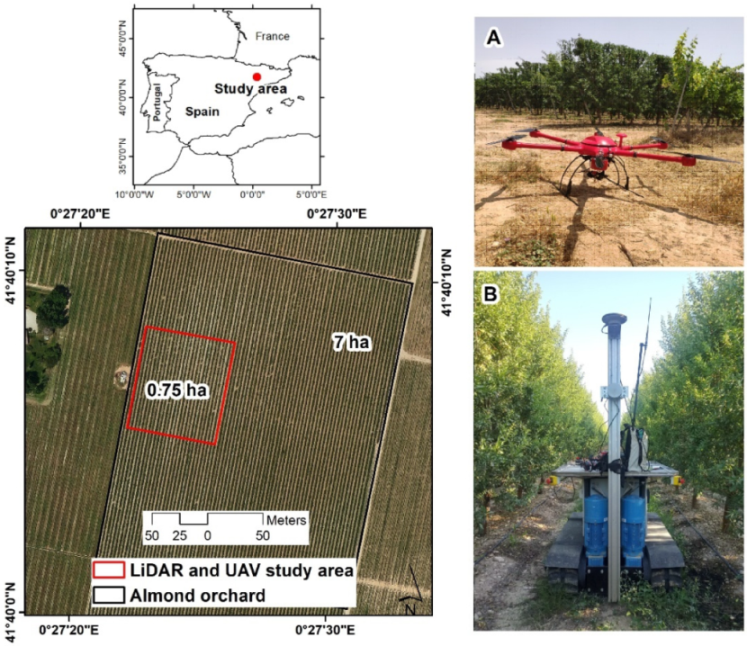
A 0.75 ha block of an almond orchard (
Prunus dulcis ‘Lauranne Avijo’) located in Raimat (Catalonia, Spain) (Lat 41°40′05″, Long 0°27′30″ WGS84) was selected as the experimental area (
Figure 1). This orchard has a pattern of 3.2 m × 1.5 m (2800 trees ha
−1, with the trees forming hedgerows (
Figure 1). Data were acquired in June 2019, after mechanical pruning in the spring.
2.2. Methodological Procedure
The methodological procedure used was as follows. First, LiDAR data were acquired along the almond hedgerows to characterize the tree architecture with geometrical parameters such as width, height and cross-sectional surface. In addition, porosity (related to foliar density) was measured from LiDAR data as the ratio between the number of impacts and the number of emitted laser beams. Different vegetation indices were then calculated from a UAV image in order to analyze their ability to estimate these parameters and to define potential MZs. For this purpose, simple and canonical correlation analyses were performed. Subsequently, a protocol to summarize vegetation index data and to interpolate a continuous map from which to derive classes for the case of a hedgerow orchard was also developed. Finally, the geometric and structural canopy parameters were tested for potential MZ differentiation by means of ANOVA tests.
2.3. LiDAR Data Acquisition and Processing
LiDAR data were acquired on 22nd June 2019, using a VLP-16 sensor (Velodyne Lidar Inc., San José, CA, USA). This device emits 16 simultaneous laser beams, with a 360° scanning window and a 30° field of view, providing ~300,000 points per second. The sensor has dual return capability and a range of 100 m. To georeference these data, a GPS 1200 GNSS-RTK system (Leica, Wetzlar, Germany) was used. As shown in
Figure 1, the LiDAR was mounted on a mobile platform which had a constant speed of 2 km h
−1.
Twenty-four tree rows (each 84 m long) were scanned during the LiDAR survey. This represented a total number of 469 million points. This point cloud was processed by means of an R code developed by the authors and described in [
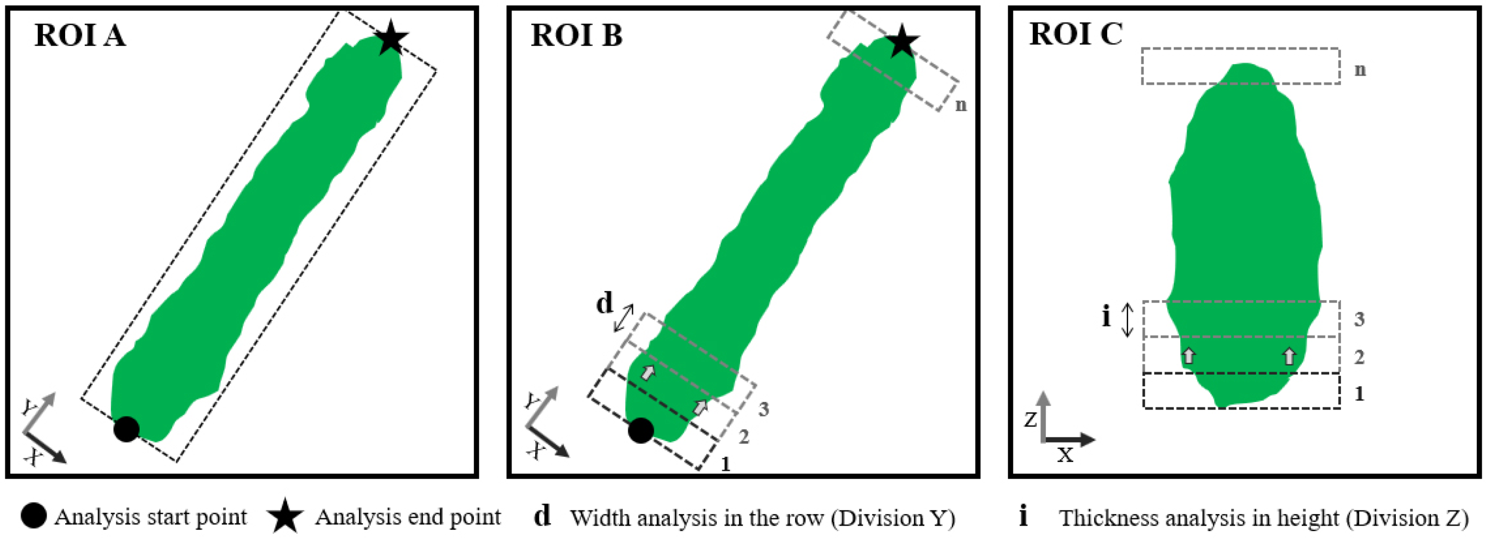
27], using RStudio (Version 1.2.5001 with R version 3.6.1). This served to extract structural and geometric parameters of the canopy every 0.5 m along the tree rows. For that (see
Figure 2), first, the coordinates of the beginning and end of each ROI-A (region of interest A) were determined. Then, the algorithm was run according to ROIs of 0.5 m increments along the
Y axis (ROI-B) and 0.10 m increments along the
Z axis (ROI-C). Due to the huge amount of data acquired, only the points generated by the central LiDAR beam were used.
Table 1 presents the structural and geometric parameters extracted with this method.
Table 1.
Structural and geometric canopy parameters extracted from the LiDAR point cloud every 0.5 m along the tree rows. See representation in
Figure 3.
Table 1.
Structural and geometric canopy parameters extracted from the LiDAR point cloud every 0.5 m along the tree rows. See representation in
Figure 3.
| Parameter | Description |
|---|
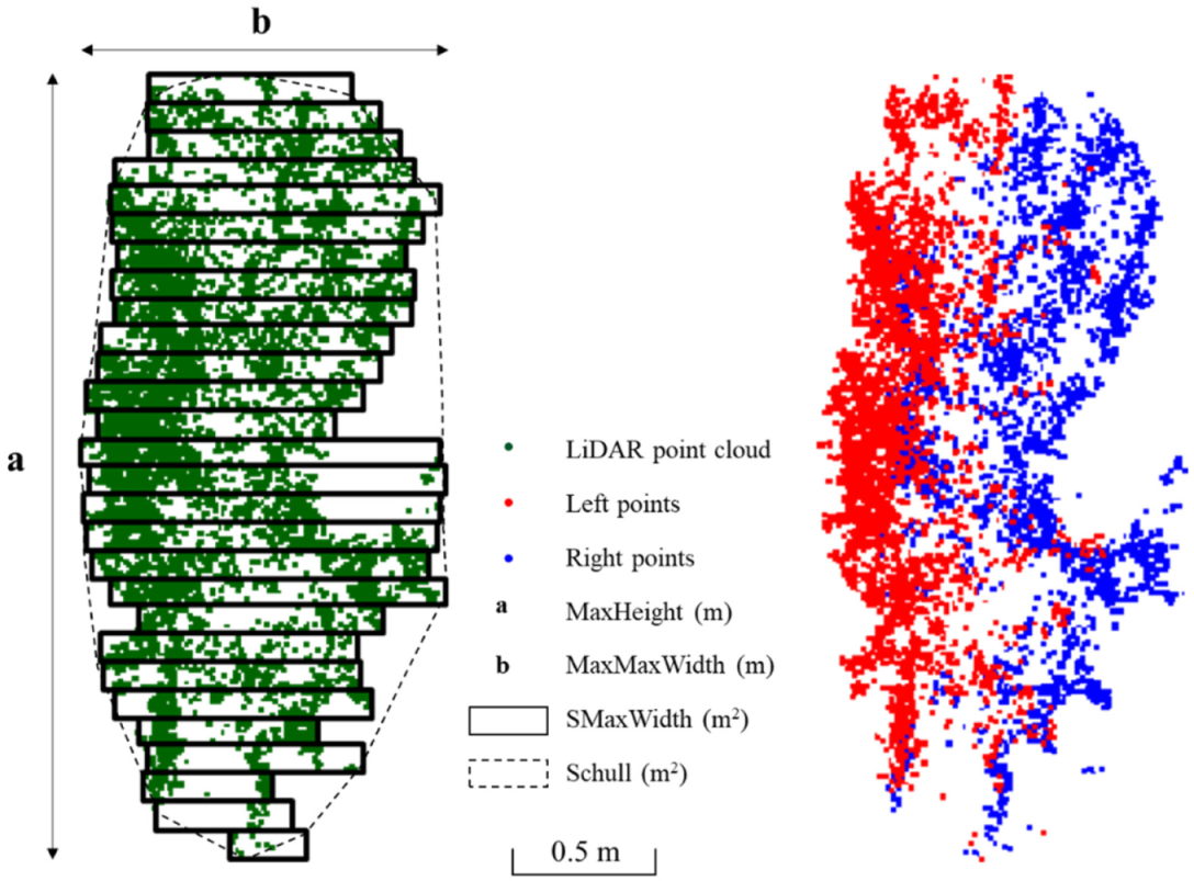
| MaxWidth (m) | Average width of the vegetation: calculated taking into account the maximum widths in each ROI-B along the Z axis (ROI-C of 0.1 m). |
| MaxHeight (m) | Maximum height of the canopy along the Z axis. Parameter “a” in Figure 3. |
| Schull (m2) | Canopy section in each ROI-B: calculated using the convex hull method (function of grDevices package in R). Surface inside the dotted line in Figure 3. |
| SMaxWidth (m2) | Sum of the rectangular cross-sections along the Z axis: calculated according to the maximum width measured at each 0.1 m along the Z axis. |
| Porosity from the Left, from the Right and Average (%) | Calculated as the ratio between LiDAR beams crossing the canopy and the beams emitted by the sensor. The average is calculated from the left and right porosity values. |
2.4. UAV Image Acquisition and Vegetation Indices
On June 26th, 2019, a multispectral image was acquired by means of a UAV. The UAV, a DroneHexa (DroneTools, Sevilla, Spain), was operated by MDrone (Barcelona, Spain). The mounted camera was a RedEdge-MTM (Micasense, Seattle, WA, USA). This camera acquires five bands: blue (475 ± 20 nm), green (560 ± 20 nm), red (668 ± 10 nm), red edge (717 ± 10 nm) and near-IR (840 ± 40 nm). The total number of photographs acquired was 306, with a resolution of 0.07 m per pixel. For the radiometric calibration, Micasense reflectance panels were used. Absolute reflectance comprised between 0.0 and 1.0, in the range of 400–850 nm. The images were processed and built in a mosaic using OpenDroneMap (Cleveland Metroparks, Cleveland, OH, USA).
Five vegetation indices were selected because of their use in the characterization of vegetation and of the possibility of being computed from the acquired multispectral images: the canopy chlorophyll content index (CCCI), the normalized difference red-edge index (NDRE) [
28], the normalized difference vegetation index (NDVI) [
10], the green normalized vegetation index (GNDVI) [
29] and the wide dynamic range vegetation index (WDRVI) [
30]. The CCCI is calculated as the ratio between the NDRE and the NDVI, with the NDRE being an estimator of N concentration [
28] and the NDVI being sensitive to low chlorophyll concentrations, to the fraction of vegetation cover and, as a result, to the absorbed photosynthetically active solar radiation [
31]. However, the NDVI does not have a linear relationship with higher chlorophyll concentrations, approaching saturation asymptotically under conditions of moderate-to-high aboveground biomass [
30]. For that reason, the GNDVI, with a better correlation between the reflectance at 550 nm and the chlorophyll concentration than when using the reflectance at 675 nm, was also considered. The sensitivity of the NDVI to high biomass conditions can be enhanced by introducing a weighting coefficient that increases the correlation with vegetation fraction by linearizing the relationship. This modification to the WDRVI was introduced by Gitelson [
30] and was incorporated in the present work. More detailed information on these indices can be found at
https://www.indexdatabase.de (accessed 22 December 2021).
2.5. UAV Image ROIs for the Comparison of Vegetation Indices with Structural and Geometric Orchard Parameters from LiDAR-Derived Data
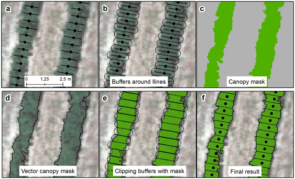
To compare the structural and geometric orchard parameters derived from LiDAR data with the vegetation indices, the following protocol was applied (see
Figure 4):
- (1)
First, and every 0.5 m along the hedge tree rows, perpendicular straight lines were generated. The lines passed by the LiDAR summary points;
- (2)
Buffer areas of 0.25 m radius were created around each line;
- (3)
A mask of the projected hedgerow canopy was created by means of supervised classification of the multispectral image;
- (4)
The mask of the projected canopy was vectorized;
- (5)
The previous buffers were clipped by the mask of the projected canopy;
- (6)
The clipped buffers were used as zones to summarize the vegetation indices;
- (7)
The areas of the clipped buffers were used to normalize the mean values of the indices in those areas. This normalization consisted of multiplying each mean vegetation index value by the area of each adjusted buffer. The normalized indices were named nCCCI, nGNDVI, nNDRE, nNDVI and nWDRVI.
2.6. Statistical Analysis
A variety of statistical methods were used to assess the relationship between vegetation indices and LiDAR-derived geometrical and structural orchard parameters: (a) an exploratory analysis of the variables by means of descriptive statistics; (b) a multivariate descriptive analysis to obtain the matrix of Pearson’s linear correlation coefficients; (c) a canonical correlation analysis to study the relationship between the two sets of variables (LiDAR-derived orchard parameters and vegetation indices); (d) a geostatistical interpolation to create the continuous spatial distribution of selected vegetation indices; (e) a cluster analysis of the continuous vegetation indices maps; and finally, (f) an analysis of variance (ANOVA) to check if classes arising from the clustering of vegetation indices allowed for effective MZs in terms of differentiating the foliar canopy in almond trees.
JMP Pro 15 (SAS Institute Inc., Cary, NC, USA), RStudio 1.4.1717 with R version 4.1.1, ArcGIS Desktop 10.8 (ESRI, Redlands, CA, USA), PAT-Precision Agricultural Tools [
32] integrated in QGIS 3.16 and VESPER [
33] software were used to carry out all these analyses.
The canonical correlation analysis, the geostatistical interpolation, the clustering and the ANOVA are explained in more detail in the following sections.
2.6.1. Canonical Correlation Analysis
To study the relationship between the two sets of variables (LiDAR-derived parameters and vegetation indices) a canonical correlation analysis was performed. A canonical correlation analysis is a generalization of multiple regression in which several Y variables are simultaneously related to several X variables [
34]. In the present case, the analyzed datasets were set X, formed by the seven geometrical and structural orchard parameters, and set Y, formed by the five normalized vegetation indices. The objective of this analysis was to detect latent relationships that could not directly be observed. Canonical correlation analysis creates an internal structure which is useful in analyzing the strength of association between the two sets of variables.
2.6.2. Geostatistical Interpolation of Vegetation Index Values
From the previous correlation analyses, the vegetation index with the best performance was selected to create a continuous surface with the objective of establishing different classes from which to distinguish zones with differentiated geometric and/or structural canopy properties. For that, a geostatistical interpolation was first performed using local block kriging implemented in the PAT-Precision Agricultural Tools [
32] integrated in QGIS 3.16, in combination with VESPER software.
First, an empty block raster grid of 2 × 2 m, onto which the variable was interpolated, was created. This is the recommended resolution to interpolate variables measured in row crops [
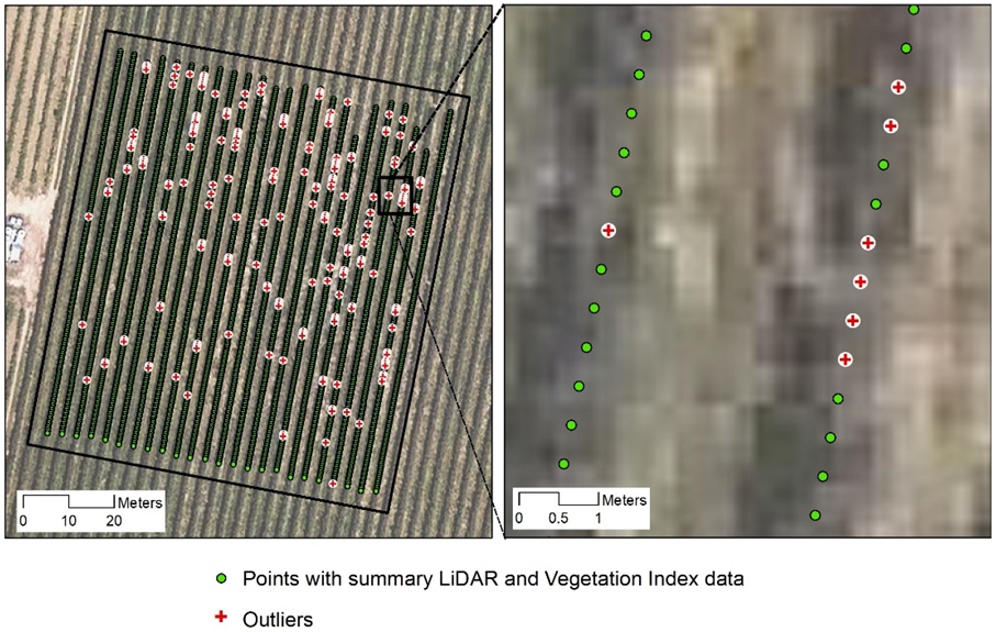
32]. Then, the point dataset with the selected vegetation index was cleaned and normalized. For that, and according to the criteria proposed by Taylor et al. [
35], the normalized data were trimmed to ±2.5 standard deviations in an iterative process to remove outliers (
Figure 5). This process removed 204 points (centroids of the ROI-B areas) out of the total 4027 original points.
From the cleaned set of points, block kriging with local variograms was applied. According to the criteria of Ratcliff et al. [
32], a block size of 10 m (five times the pixel resolution) was considered.
2.6.3. Clustering and Analysis of Variance for the Definition of Potential Management Zones
After the interpolation, the resulting vegetation index map was clustered in two and three classes using the k-means algorithm [
36] implemented in the PAT-Precision Agriculture Tools plugin for QGIS. This algorithm assigns each pixel to the nearest cluster mean (cluster centers). This tool creates clusters which minimize variability within clusters while maximizing variability between them. If significant differences between clusters are observed, then the clustered results can be used as potential MZs [
32]. Then, to check for significant differences in structural and geometric orchard parameters according to clusters, an ANOVA was carried out. For that, each centroid point where those parameters were referred to was classified according to its spatial location, assigning to it the cluster number where the point was included. In the present case, the ANOVA provided a statistical test of whether 2 or 3 population means were equal. In the case that the null hypothesis was rejected, a Student’s t-test (in the case of 2 clusters) or a Tukey’s HSD (honestly significant difference) test (in the case of 3 clusters) was performed in order to compare the means and check for statistical differences between the average values of the geometric and structural orchard parameters. JMP Pro 15 software was used to perform this analysis.
4. Discussion and Conclusions
The objective of the present work was to contrast the hypothesis of the existence of significant relationships between structural and geometric parameters of hedgerow almond orchards with vegetation indices derived from UAV-acquired images. If confirmed, this could serve as a basis for the delineation of MZs.
As reviewed in the Introduction, very few studies have been published about the delineation of differential MZs in orchards, and none in relation to LiDAR-acquired data. In this work, we have confirmed the existence of significant relationships in a hedgerow almond orchard by means of different statistical analyses, which opens the possibility to delineate MZs on the basis of vegetation index data.
Methodologically, this article introduces a protocol to summarize and interpolate vegetation indices in hedgerow fruit tree orchards, as in the case study example. This method is different from that previously used by Uribeetxebarria et al. [
2], who summarized and interpolated vegetation indices from individual trees in a peach orchard. In addition, the indices were calculated from an airborne image as opposed to a UAV image. Nevertheless, in the present case, as well as in Uribeetxebarria et al. [
2], the projected canopy area served to normalize the values of the vegetation indices, otherwise small but vigorous trees would have the same weight as bigger trees with similar vigor. Another difference with respect to other studies working on the delineation of MZs in orchards was that the present proposed method is exclusively based on weighted vegetation indices. This is different from the approaches of Aggelopooulou et al. [
4] or Oldoni et al. [
5], who based the delineation of MZs on soil and crop (yield and quality) data in an apple and a pear orchard, respectively. Other authors combined the clustering of individual trees by means of the Getis–Ord Gi* statistic algorithm with
k-means multivariate clustering [
7], with this method being more suitable for orchards with traditional plantation patterns.
Regarding the correlation analysis between structural and geometric orchard parameters and the normalized vegetation indices, the highest correlations (r ≥ 0.70) were found between MaxWidth and SMaxWidth and nNDVI (r = 0.70 and 0.73, respectively), and between SmaxWidth and nGNDVI (r = 0.70). These are logical relationships, because the UAV image offers a zenithal view of the tree rows which contrasts with soil reflectance between the rows, clearly defining the tree row width in each section. This is consistent with the findings of different authors who characterized geometrical properties by means of either RGB or multispectral images from UAVs extracted by photogrammetric processes [
20,
21,
37], among others.
Negative correlations (up to r < −0.50) were found between porosity and the normalized vegetation indices. Porosity is an important structural variable that can be used to describe radiation penetration through the tree. The results in the present study confirmed its high variability (between 6.28% and 67.13% on average, CV = 0.33,
Table 3). Other different studies which quantified tree crown porosity found similar results [
38,
39]. However, the geometric properties presented much lower coefficients of variation (between 0.04 and 0.14), probably due to the mechanical pruning of the orchard, which aims to constrain the tree canopy in a rectangular parallelepiped. This was particularly the case of MaxHeight, which showed no correlation with either the other geometrical variables or the vegetation indices.
The results of the canonical correlation analyses confirmed the above-mentioned relationships, with a preference for the nNDVI as the index with the highest correlation with geometrical and structural parameters (
Table 3). This modified vegetation index presented a Cambardella index (CI) [
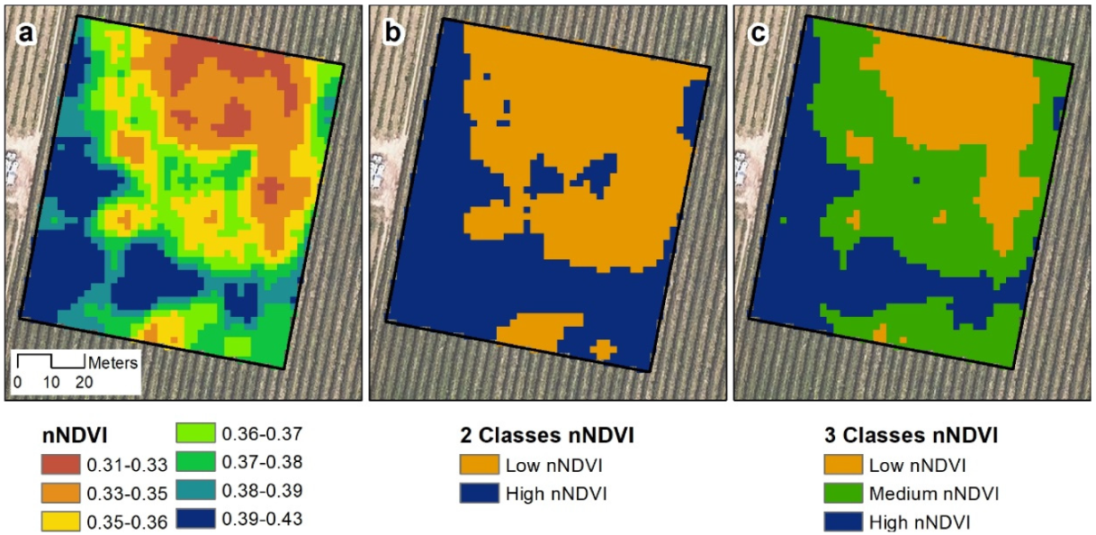
40] of 23.5%, indicating a high degree of spatial autocorrelation within the plot. From this index, two and three nNDVI classes were created, reflecting a clear spatial pattern (
Figure 6). In the case of two classes, all the variables were differentiated in distinct groups, but not all in the case of three classes. In the latter case, only the MaxHeight, Schull and SMaxWidth properties, which had the highest correlation with nNDVI, presented differentiation in the three classes, i.e., two-zone differentiation of geometrical and structural orchard parameters could be better than three-zone differentiation. These results agree with experiences in other 3D row crops such as grapevine in the same study area [
41]. These authors found that differentiation into two vigor zones was preferable because of occasional ambiguity when classifying the medium/moderate-vigor zone. In the present case, this occurred with MaxWidth and Porosity, which only showed a clear differentiation in two classes. Nevertheless, those parameters presented a logical gradation of the average values in the three classes, although with total differentiation. Thus, and according to Ratcliff et al. [
32], the classes delimited by the cluster analysis could be used as potential MZs, with a preference for delineating two MZs instead of three in the present case.
Although significant differences in the structural and geometric parameters were found between the nNDVI classes (
Table 7), the average values of the classes were very close: a few centimeters in the case of width and height, or between 1.27 and 1.33 percentual values in the case of porosity. Further studies are required to determine the extent to which these small differences in structural and geometric properties of the canopy can result in differences in orchard productivity. These small but significant differences could have been influenced by the timing of the study (after pruning). Nevertheless, the results highlight the necessity to work on two additional lines: (i) the introduction of productive and/or quality analyses to determine the extent to which the differences are agronomically significant; and (ii) determination of the optimal spatial resolution on which to base the data acquired within the plantations. It also remains to be answered whether such vast quantities of data at very high resolution are required for optimal orchard management.
Vegetation indices from either UAV multispectral images have mainly been used to estimate leaf chlorophyll and other biophysical parameters, such as the LAI to monitor tree vigor, disease detection or to predict yield in orchards [
8,
25,
37,
42,
43]. Nevertheless, and according to [
25], the use of UAVs is largely underutilized in orchard management. In this respect, the results of the present research expand the possibilities of using multispectral images in orchard management and, in particular, in hedgerow plantations. Therefore, orchards of species other than almonds, such as apples, pears, peaches, apricots, plums and even olives (among others) arranged in hedgerow patterns could benefit from the methodology presented in this article. In addition, this methodology can be useful to extend MZ delineation to large orchards where the huge amount of data generated by MTLS sensors could be a bottleneck for its practical applications.


 ,
, 


