Article

Evaluation of NASA POWER Reanalysis Products to Estimate Daily Weather Variables in a Hot Summer Mediterranean Climate

by
Gonçalo C. Rodrigues
1,2,* and
Ricardo P. Braga
1,2
1
LEAF—Linking Landscape, Environment, Agriculture and Food—Research Center, Instituto Superior de Agronomia, Universidade de Lisboa, Tapada da Ajuda, 1349-017 Lisboa, Portugal
2
Instituto Superior de Agronomia, Universidade de Lisboa, Tapada da Ajuda, 1349-017 Lisboa, Portugal
*
Author to whom correspondence should be addressed.
Agronomy 2021, 11(6), 1207; https://doi.org/10.3390/agronomy11061207
Submission received: 11 May 2021 / Revised: 7 June 2021 / Accepted: 11 June 2021 / Published: 14 June 2021
(This article belongs to the Special Issue Water Saving in Irrigated Agriculture)

Abstract

:
This study aims to evaluate NASA POWER reanalysis products for daily surface maximum (Tmax) and minimum (Tmin) temperatures, solar radiation (Rs), relative humidity (RH) and wind speed (Ws) when compared with observed data from 14 distributed weather stations across Alentejo Region, Southern Portugal, with a hot summer Mediterranean climate. Results showed that there is good agreement between NASA POWER reanalysis and observed data for all parameters, except for wind speed, with coefficient of determination (R2) higher than 0.82, with normalized root mean square error (NRMSE) varying, from 8 to 20%, and a normalized mean bias error (NMBE) ranging from –9 to 26%, for those variables. Based on these results, and in order to improve the accuracy of the NASA POWER dataset, two bias corrections were performed to all weather variables: one for the Alentejo Region as a whole; another, for each location individually. Results improved significantly, especially when a local bias correction is performed, with Tmax and Tmin presenting an improvement of the mean NRMSE of 6.6 °C (from 8.0 °C) and 16.1 °C (from 20.5 °C), respectively, while a mean NMBE decreased from 10.65 to 0.2%. Rs results also show a very high goodness of fit with a mean NRMSE of 11.2% and mean NMBE equal to 0.1%. Additionally, bias corrected RH data performed acceptably with an NRMSE lower than 12.1% and an NMBE below 2.1%. However, even when a bias correction is performed, Ws lacks the performance showed by the remaining weather variables, with an NRMSE never lower than 19.6%. Results show that NASA POWER can be useful for the generation of weather data sets where ground weather stations data is of missing or unavailable.

1. Introduction

Weather variables are regarded as one of most significant factors affecting decision making in agriculture. In many regions around the world, weather variables are not observed, are of poor quality due to lacking quality control, or are not available for free. Reanalysis and gridding meteorological data from global atmospheric models are considered as one of weather data sources that can be used to compensate lack of observation, quality, or availability [1].
Reanalysis of the observations, with more complete data, improved quality control, and with constant state-of-the-art assimilating models and analysis systems, greatly improves the homogeneity of the record and makes it useful for examining weather variations. This whole endeavor is now referred to as “reanalysis” [2]. The reanalysis products are constructed from numerical weather data assimilation systems that use a variety of atmospheric and sea surface observations to provide for long-term atmospheric and land surface variables [3]. However, some reanalysis products may require corrections using observation-based datasets in order to amend for anomalies that arise from land surface modelling [4].
There are several historical reanalysis datasets available, such as the Climate Forecast System Reanalysis (CFSR) [5], the ERA-Interim reanalysis products [6], provided by the European Centre for Medium-Range Weather Forecasts (ECMWF), the Japanese Meteorological Agency (JRA-55), [7], the National Center for Environmental Prediction/National Center for Atmospheric Research (NCEP/NCAR) [8], the NASA Modern Era Retrospective-Analysis for Research and Applications (MERRA) [9] and NASA Prediction of Worldwide Energy Resource (NASA POWER) [10]. The latter, available for a resolution of 0.5° latitude by 0.5° longitude at the NASA POWER’s website (https://power.larc.nasa.gov/, accessed on 1 November 2020), provides daily data of near surface air temperature, relative humidity, rainfall, solar radiation and wind speed and direction. All datasets derive from using simulations of numerical weather prediction models based on a set of meteorological observations. However, the ease of use of NASA POWER allows to easily access data since it is available as a single point, providing regional and global coverage with daily, interannual and climatological temporal averages. By selecting a single point, a time series of data is made available based on the registered coordinate—single latitude and longitude. The regional endpoint produces a time series dataset based on a bounding box of latitude and longitude coordinates defined by the user. The global endpoint returns long-term climatological averages for the entire globe. If data proves to be accurate, its user-friendly interface allows any end-user to easily have access to near-real time sound weather data from anywhere around the globe.
Many studies evaluated the accuracy of most weather variables from the available reanalysis datasets such the CFSR [11,12,13,14], the ERA-Interim [11,15,16,17], the JRA-55 [14,17,18], the NCEP/NCAR [11,19,20] and the MERRA [14,21,22]. Nevertheless, few studies aimed to evaluate the performance of NASA POWER data.
White et al. [23] compared daily temperature from NASA POWER in the continental USA, concluding that the reanalysis data showed good agreement with a root mean square error (RMSE) of 4.1 °C for maximum temperature and 3.7 °C for minimum temperature. Additionally, they recommended that data could be improved by adjusting for elevation effects, reducing seasonal bias, and refining estimation of actual maximum and minimum temperatures in diurnal cycles. Bai et al. [24] assessed NASA POWER’s daily maximum and minimum temperatures and solar radiation in China. They concluded that there is a close relation between NASA POWER and the observed data with a RMSE of 4.0 °C, 3.2 °C and 3.4 MJ m–2 d–1 for maximum and minimum temperatures, and solar radiation, respectively. Negm et al. [25] assessed the suitability of NASA POWER to estimate reference evapotranspiration through daily maximum, minimum and average air temperatures, relative humidity, global solar radiation and wind speed, in Sicily, Italy. Results showed a RMSE for those variables, respectively of 3.6 °C, 5.0 °C, 3.2 °C, 12.2%, 2.7 MJ m–2 d–1 and 2.4 m s−1, allowing them to conclude that NASA POWER had agreement with the corresponding measured values on ground weather stations. However, inaccurate estimations of relative air humidity occurred for the coastal weather stations. Monteiro et al. [26], performed a similar study in Brazil, found similar agreement for the same variables. Aboelkhair et al. [1] evaluated NASA POWER reanalysis data for surface monthly average maximum, minimum, average and dew point temperatures, and relative humidity in comparison the observed data in Egypt. The results showed that there is a significant correlation between NASA POWER reanalysis and observed data for all temperature parameters (RMSE lower than 5 °C) but failed to accurately simulate relative humidity (with an average RMSE of 11.6%). However, none of those previous studies evaluated the impact of bias correction on reanalysis products.
Using daily meteorological NASA POWER reanalysis data and observations from 14 weather stations in Alentejo region, Southern Portugal, the objectives of this study are: (1) assess the accuracy of NASA POWER maximum and minimum temperatures, solar radiation, relative humidity and wind speed when compared to local observations; (2) assess the performance of alternative bias correction procedures to improve reanalysis accuracy.

2. Materials and Methods
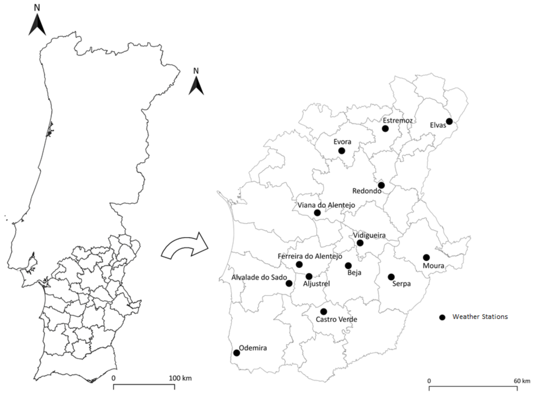
2.1. Study Area

This study was conducted in Alentejo Region, Southern Portugal. The region has a Köppen–Geiger Csa climate, and is characterized by a semi-arid Mediterranean climate of hot and dry season in the summer and mild temperature associated to annual rainfall in winter. This region was selected due to its characteristics, being semi-arid and prone to desertification, where water availability is crucial to achieve farming sustainability and profitability. Additionally, and due to recurrent water scarcity, this agricultural area is prone to several risks associated with weather.
Daily meteorological data from 14 ground weather stations were obtained from the Irrigation Operation and Technology Center (COTR). The number and location of the selected weather stations allow to evaluate the performance of the reanalysis data at the regional level, and to better understand the spatial–temporal trends of the series. All weather data are validated every day by a team of experienced technicians, assuring its quality and feasibility. Figure 1 and Table 1 present, respectively, the geographical position of the weather data locations, their coordinates and period of observation.

2.2. Agroclimatic Data

The annual mean and standard deviation for the selected weather variables—maximum and minimum temperature, solar radiation, relative humidity and wind speed—are shown in Table 2. These data were interpolated between stations to cover all Alentejo region, as illustrated in Figure 2, using kriging algorithm. Due to the specific nature of the atmospheric processes leading to rainfall, we left the evaluation of this variable to a dedicated study. The same weather parameters for the same period of observations were collected from NASA POWER from the nearest grid point of the target location.
Figure 2 shows that the Atlantic Ocean (and somewhat the proximity the Mediterranean Sea) plays a significant role in the temperature, humidity and wind speed variations across the region. The locations closer to the sea (e.g., Odemira) present lower temperature amplitudes (with lower maximum and higher minimum average temperatures) and higher relative humidity and wind speed. On the other hand, at more inland locations (e.g., Moura), temperature tends to present higher maximums and lower minimums, with lower relative humidity and wind speed. Therefore, there is an inverse relationship between average temperature and relative humidity. Solar radiation tends to increase with lower latitudes.

2.3. Evaluation Criteria

The estimation accuracy of each variable was assessed through the metrics listed below, where Oi and Pi (i = 1, 2, …, n) represent pairs of values of each variable using locally collected data and the NASA POWER estimated data, respectively, and   O ¯   and   P ¯   are the respective mean values and n is the number of samples of each variable:
  • The coefficients of regression and determination, relating the observed and simulated data, b and R2, respectively, are defined as:
b = i = 1 n O i P i i = 1 n O i 2
R 2 = i = 1 n O i     O ¯ P i     P ¯   i = 1 n O i O ¯ 2 0.5 i = 1 n P i P ¯ 2 0.5 2
Henseler et al. [27] defines that R2 values of 0.25, 0.50 and 0.75 match weakly, moderately and significantly fit, respectively.
  • The root mean square error, RMSE, and its normalization, NRMSE, which characterizes the variance of the estimation error:
RMSE = i = 1 n O i     P i 2 n 0 . 5
NRMSE   = RMSE O ¯ × 100 %
RMSE measures overall discrepancies between observed and estimated values and the smaller, the better accuracy. NRMSE is dimensionless, allowing to compare its values for different variables, assuming a good goodness of fit with a normalization below 15%.
  • The mean bias error, MBE, and its normalization, NMBE, that measures the systematic error between the predicted and observed values:
MBE = i = 1 n P i O i n
NMBE = MBE O ¯ × 100 %
The MBE and NMBE measure if the predicted data is over or under estimation with its positive or negative values, respectively. MBE intends to indicate the average interpolation bias [28].
  • The Nash and Sutcliffe [29] modelling efficiency, EF, that is the ratio of the mean square error to the variance in the observed data, subtracted from unity:
EF = 1 . 0 i = 1 n O i P i 2 i = 1 n O i O ¯ 2
As suggested by Legates and McCabe [30], if the square of the differences between model simulations and observations is as large as the variability in the observed data, then EF tends toward 0.0 and the O mean,   O ¯ , is as good a predictor as the model, while negative values indicate that   O ¯ , is an even better predictor than the model. EF can vary between −∞ and 1.

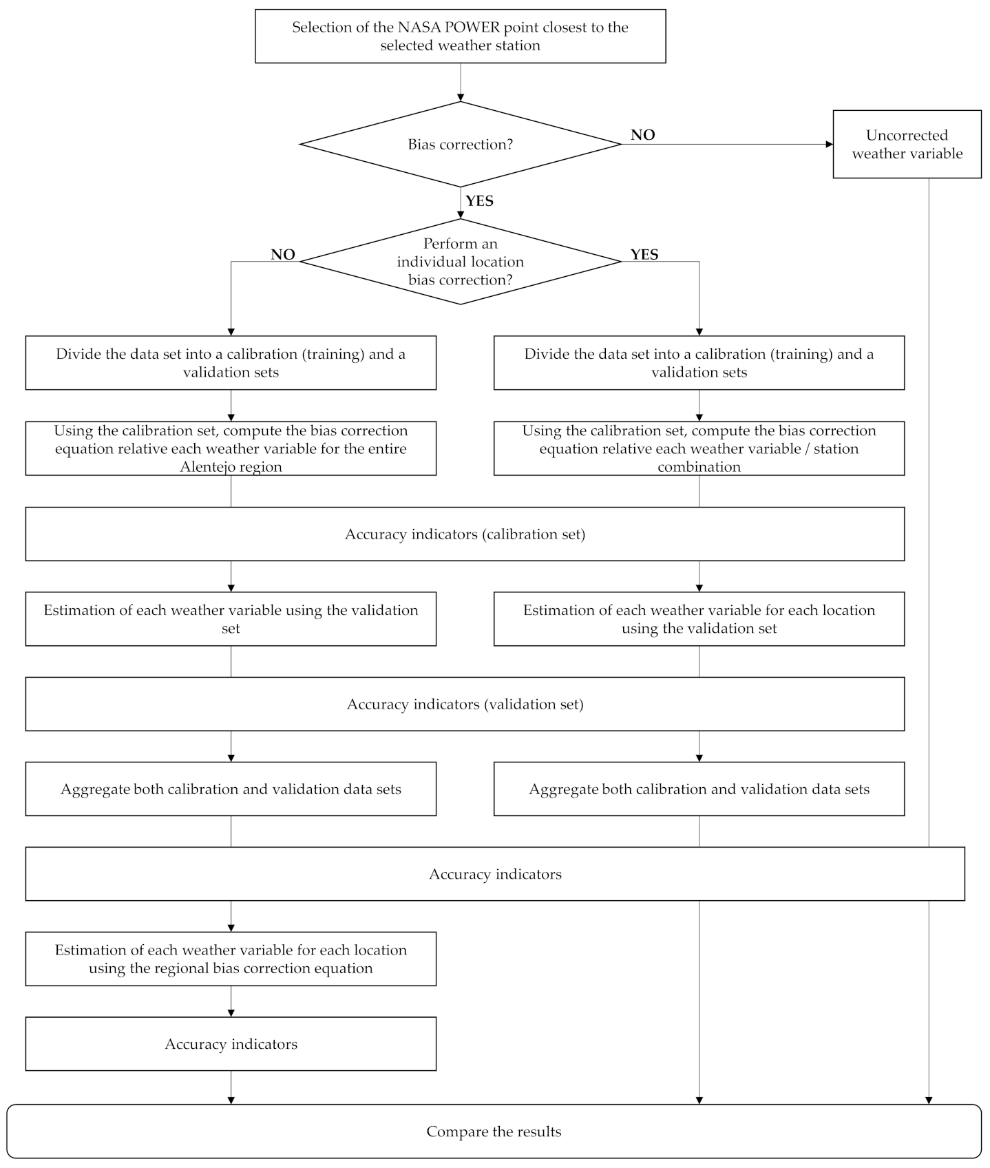
2.4. Correction of Bias

Bias correction seeks to reduce the differences between the NASA POWER data and the observed data, since forecast products are often biased due to errors in the host weather forecast models [31]. To find an accurate yet simple bias correction procedure, the approach proposed by Leander and Buishand [32], where the correction of bias only involves shifting and scaling to adjust the mean and variance, was used. Two bias corrections schemes were carried out for each variable (Figure 3): (1) for the Alentejo Region as a whole, hereby defined as a regional bias correction, where all data was treated as one set; (2) for each location individually, defined onwards as a local bias correction.
For each scheme, the corrected daily weather variable X’ was obtained as:
X = X Obs   ¯ + σ X Obs σ X NASA ×   ( X NASA   -   X Obs ¯ )   +   ( X Obs ¯   -   X NASA ¯ )
where XNASA is the uncorrected NASA POWER’s daily weather variable and Xobs is the observed daily weather variable. In the equation an overbar denotes the average over the considered period and σ the standard deviation. The ratio of the standard deviation performs the scaling while the difference of the averages performs the shifting of bias.
A major uncertainty of bias correction refers to how well it performs for conditions different from those used at calibration. Thus, a validation procedure was applied, consisting in providing a validation of model fit with a set of data that is independent of the model fitting set. In the present study, the models were fitted individually for each weather station location and validated on independent data sets for the same location. The validation procedure consisted in dividing each data set into two subsets of the same size, randomly chosen from the dataset (e.g., Paredes et al. [16]). For each iteration, the first set was used for calibration and the second was used for validation (Figure 3). Equation (1) parameters were obtained from the calibration dataset, and then used with the validation dataset. The assessment of the performance of each bias correction procedure was performed on the calibration and validation sets. When comparing the accuracy metrics of bias corrected calibration and validation datasets with the bias corrected full datasets, no evidence of overfitting was found, with the estimated parameters only showing residual differences (Supplementary Tables S1–S5). Thus, in order to test the validity of the procedure when applied to long sets, the approach to bias correct the full dataset was hereby adopted.

3. Results

3.1. Bias Correction Equations

The resulting calibrated and validated bias correction equations, following the procedure presented in Figure 3, are presented in Table 3. The results obtained when adopting each equation are presented int the following Sections. Full results for all locations, with and without bias corrections, are presented in Supplementary Tables S1–S5.

3.2. Evaluation of Maximum Temperature Accuracy

Table 4 presents the mean and range values of the accuracy metrics relative to NASA POWER maximum temperature with and without bias correction. Results show that NASA POWER successfully simulate maximum temperature data, with an excellent accuracy, even if no bias correction is performed, with a R2 and EF higher than 0.82 and 0.68, respectively, a mean NRMSE of 7.59% and an average NMBE equal to −2.56%. If a regional bias correction is applied, results show a slightly better performance: mean b increases by 2.2% (to 1.00), while the average RMSE decreases 9.2% (1.74 °C day–1), and the mean MBE increases 104.4% (to 0.03 °C day–1). Similarly, if a local bias correction is adopted, the accuracy metrics tend to improve with the mean RMSE, MBE and EF: the mean root mean square error decreases 17.0% (RMSE = 1.59 °C day–1), the average mean bias error decreases 97.5% (MBE = −0.02 °C day–1) and the mean modelling efficiency increases by 2.8% (EF = 0.95).
Results (Supplementary Table S1 and Figure S1) show that only 14% of the weather stations show an NRMSE ≤ 6.5% if no bias correction, contrasting with the results obtained when a local bias correction is performed where 57% of the weather stations present an NRMSE ≤ 6.5%. When no bias correction is performed, 28% of the weather stations show an NMBE ranging −2.5 to 2.5%; however, when a correction is applied, for the same NMBE range, the frequency increases to 71 and 100%, for regional and local bias correction, respectively. Additionally, if Tmax is locally bias corrected, an EF higher that 0.95 is obtained for 79% of all locations; if no bias correction is performed, only 29% of the location perform equally.

3.3. Evaluation of Minimum Temperature

Mean and range values of the accuracy metrics relative to minimum temperature (Table 5) show that NASA POWER can successfully estimate daily Tmin data with a R2 higher than 0.85, showing an excellent accuracy of NASA POWER when compared with observed data. These results were obtained when adopting the calibrated and validated bias correction equations presented in Table 3. If no bias correction is performed, minimum temperature can be estimated with an EF averaging 0.84, with a mean RMSE of 2.01 °C day–1 and a mean MBE of 1.03 °C day–1. Results tend to improve when a bias correction is applied: for a regional correction, mean b decreases by 8.9% (to 0.99), while the mean RMSE and MBE show a decrease of 16.4% (to 1.68 day–1) and 105.2% (to −0.05 °C day–1), respectively; if a local bias correction is applied, the average RMSE is even lower (with a decrease of 21.3% to 1.58 °C day–1) with mean MBE equal to −0.02 °C day–1, representing a decrease of 101.8% when compared with raw data. The modelling efficiency tends to increase on both correction schemes to an average 0.89 and 0.90 for regional and local bias correction, respectively.
If no bias correction is performed, 86% of the weather stations show an NRMSE higher than 18%. If the bias of Tmin is regionally corrected, the most frequent NRMSE ranges from 22 to 26% (36% of all weather stations), while when a local bias correction is performed 57% of the weather stations present an NRMSE ≤ 18%. When no bias correction is performed, 14% of the weather stations show an NMBE ranging −5 to 5%, while if a local bias correction is applied, Tmin is estimated with an NMBE lower than ±5% for all locations. If Tmin is locally bias corrected, an EF higher that 0.84 is obtained for all locations. Full results of the accuracy metrics for minimum temperature are presented in Supplementary Table S2 and Figure S2.

3.4. Evaluation of Solar Radiation

Solar radiation (Table 6) was the most accurate NASA POWER weather variable evaluated. All stations present a R2 value higher than 0.91, as high as 0.97 for Redondo and Vidigueira (Table S3), representing an excellent accuracy. NASA POWER Rs present a RMSE lower than 2.73 MJ m–2 d–1 with a normalization of 16.12% and a mean EF of 0.93. NASA POWER tends to slight overestimate solar radiation (MBE averaging 0.65 MJ m–2 d–1). If NASA POWER Rs bias is regionally corrected, all accuracy metrics tend to increase resulting in a b, RMSE, MBE and EF averaging 1.00, 1.99 MJ m−2 day−1, −0.01 MJ m−2 day−1 and 0.94, respectively. For all locations, the accuracy metrics show an even better goodness of fit and agreement between the observed and simulated solar radiation when the bias is locally corrected with mean RMSE decreasing 10.2% (RMSE = 2.10 MJ m−2 day−1), mean MBE decreases 98.6% (MBE = 0.01 MJ m−2 day−1) and a modelling efficiency improving by 1.5% (EF = 0.94).
Therefore, errors are relatively small for Rs, with more frequent (Supplementary Figure S3) NRMSE lower than 13.5%, even without a bias correction. Additionally, the most frequent EF is higher than 0.93 for 93% of all locations, when the bias is both regionally and locally corrected; also, the most frequent NMBE ranges from −4.0 to 4.0 with and without a bias correction, showing low under or overestimation of Rs data.

3.5. Evaluation of Relative Humidity

Accuracy metrics for NASA POWER relative humidity as compared to local observations is shown in Table 7. Results, when adopting the calibrated and validated bias correction equations shown in Table 3, present a mean R2 of 0.82 (as high as 0.88). However, for Odemira (Table S4) the coefficient of determination is equal to 0.40, showing low correlation and with fit between observed and simulated RH; this may be due to the station closeness to the sea, and the influence of both Atlantic Ocean and Mediterranean Sea. The EF values average 0.61 and range from –0.08 to 0.79. Additionally, for raw NASA POWER RH data, the RMSE averages 9.24% day–1 (with an NRMSE of 13.00%), with MBE averaging –5.17% day–1(with an NMBE of –7.27%). However, the bias is corrected, results improve significantly with both correction schemes showing an increase of the mean b of 7.7% (to 1.01) and a mean EF increasing by 30.7% 8 to 0.80). The mean RMSE decreases to 28.8 and 30.0% for a regional and local bias correction, respectively, with normalizations below 9.25%. The most frequent EF (Supplementary Figure S4) for both schemes is higher than 0.80, with more than 93% of all stations having an NMBE between −1.0 and 1.0%.

3.6. Evaluation of Wind Speed

Among all the weather variables evaluated, NASA POWER’s wind speed is the least accurate. When using the calibrated and validated wind speed bias correction equations (Table 3), the maximum value of R2 (0.79) was recorded for Beja while the minimum values of R2 (0.52) was obtained for Elvas (Table S5), showing a moderate to high fit between reanalysis and observed wind speed data. Results for the uncorrected NASA POWER wind speed data (Table 8) show a mean coefficient of regression of 1.40, with an average RMSE of 1.10 m s−1, a mean NRMSE equal to 62.50% and an average modelling efficiency of −0.88. Wind speed is overestimated by NASA POWER for all weather stations, with an MBE that varies from 0.12 to 1.44 m s–1. Bias correction increases the accuracy of NASA POWER wind speed estimation significantly. The mean EF increased to 0.40 (an improvement of 146.3%), for a regional correction, and to 0.53 (an increase of 160.7%), when locally correcting the bias. The RMSE decreased 37.4% (to 0.69 m s−1), for the former, and 45.7% (to 0.60 m s−1*, for the latter. The most frequent (Supplementary Figure S5) NMBE and EF for the raw NASA POWER wind speed data is higher than 60% (42% of all locations) a lower than 0 (71% of all locations), respectively; however, if the dataset is locally bias corrected, the most frequent NMBE ranging −10.0 to 10.0%, with more than 60% of the stations showing an EF higher than 0.50.

4. Discussion

Based on the results presented we can conclude that NASA POWER is capable of predicting most weather variables accurately for the Alentejo Region. Table 9 presents the mean and standard deviation values of all the accuracy metrics relative to NASA POWER weather variables, with and without bias correction. NASA POWER’s raw maximum and minimum temperature and solar radiation show to be accurate with the high agreement and goodness of fit, with very little under and over estimations, when compared to the observations. When performing a bias correction, results tend to improve. In average, MBE values improve from −0.64 and 1.03 to −0.02 °C day–1 for Tmax and for Tmin, and from 0.65 to 0.01 MJ m−2 day−1 for Rs. Additionally, a local bias correction of NASA POWER Tmax, Tmin and Rs improved the mean RMSE values from 1.91 °C, 2.01 °C and 2.10 MJ m−2 day−1 to 1.59 °C, 1.58 °C and 1.89 MJ m−2 d−1, respectively. Similar results for those variables were found by Bai et al. [24] in China, by Monteiro et al. [26] in Brazil and by Negm et al. [25] in Italy. White el al. [23], for continental USA, and Aboelkhair et al. [1], for Egypt, also reported similar results and concluded that NASA POWER can accurately estimate maximum and minimum temperature. Therefore, the presented results show that NASA POWER can simulate maximum, minimum temperatures and solar radiation with a high goodness of fit and agreement, when compared with observed data.
NASA POWER’s relative humidity also shows good accuracy for inland locations when compared with observed data with, after bias correction, an average RMSE and MBE of 6.47% day–1 and 0.78% day–1, respectively. This represent an improvement from raw RH data, where a mean RMSE of 9.24% day–1 and a mean MBE of −5.71% day–1 were found. However, for coastal stations the estimation still needs improvement. Similar conclusions were drawn by Negm et al. [25], Monteiro et al. [26] and Aboelkhair et al. [1]. Nonetheless, one can conclude that NASA POWER can simulate RH with good accuracy, when compared with observed data.
Among all weather variables, NASA POWER’s wind speed is the one that performs the worst. Raw data show RMSE and MBE values averaging 1.10 and 0.85 m s−1 with a coefficient of regression equal to 1.40. Results tend to improve with a bias correction; however, the lowest NRMSE is of 19.6%, thus one can conclude that wind speed lacks the performance showed by the remaining weather variables. Previous studies [25,26,32] also found that NASA POWER fails to estimate wind speed with acceptable accuracy. Despite the improvements if a bias correction is performed, the NASA POWER wind speed reanalysis data show unsatisfactory correlation and does not agree with most of the ground observations and still needs improvement.

5. Conclusions

Weather data is one of the key elements for crop and water management. However, the quality or availability of data in remote regions is questionable. Therefore, evaluating the potential of using daily reanalysis data—such the data provided by NASA POWER—as an alternative to ground observations is needed.
The results presented in this study demonstrated that NASA POWER is capable of estimating most weather data—maximum and minimum temperatures, solar radiation—with high accuracy for Alentejo Region, Southern Portugal. Though, for wind speed and coastal relative humidity, NASA POWER estimations still need improvements. However, we suggest a local bias correction of all variables, allowing improvement to the accuracy of the estimated data. It can be concluded that NASA POWER could be useful for generation of weather data sets where ground weather stations data is missing or unavailable, improving weather information for a better decision making. Nonetheless, additional studies are recommended to better assess the use of such data for the estimation of derived products such as yield and water requirements estimations, and weather impacts on crop management and practices.

Supplementary Materials

The following are available online at https://www.mdpi.com/article/10.3390/agronomy11061207/s1: Table S1: Accuracy metrics relative to NASA POWER maximum temperature with and without bias correction for all 14 locations, Table S2: Accuracy metrics relative to NASA POWER minimum temperature with and without bias correction for all 14 locations, Table S3: Accuracy metrics relative to NASA POWER solar radiation with and without bias correction for all 14 locations, Table S4: Accuracy metrics relative to NASA POWER relative humidity with and without bias correction for all 14 locations, Table S5: Accuracy metrics relative to NASA POWER wind speed with and without bias correction for all 14 locations, Figure S1: Frequency (%) distribution of the accuracy metrics measuring the performance of NASA POWER maximum temperature (Tmax) without bias correction compared with adopting a regional bias correction and a local bias correction, Figure S2: Frequency (%) distribution of the accuracy metrics measuring the performance of NASA POWER minimum temperature (Tmin) without bias correction compared with adopting a regional bias correction and a local bias correction, Figure S3: Frequency (%) distribution of the accuracy metrics measuring the performance of NASA POWER solar radiation (Rs) without bias correction compared with adopting a regional bias correction and a local bias correction, Figure S4: Frequency (%) distribution of the accuracy metrics measuring the performance of NASA POWER relative humidity (RH) without bias correction compared with adopting a regional bias correction and a local bias correction, Figure S5: Frequency (%) distribution of the accuracy metrics measuring the performance of NASA POWER wind speed (Ws) without bias correction compared with adopting a regional bias correction and a local bias correction.

Author Contributions

Conceptualization, G.C.R. and R.P.B.; methodology, G.C.R. and R.P.B.; Data analysis, G.C.R.; Writing—Original draft preparation, G.C.R.; Writing—Review and editing, G.C.R. and R.P.B. All authors have read and agreed to the published version of the manuscript.

Funding

This work is funded by national funds through FCT –Fundação para a Ciência e a Tecnologia, I.P., in the scope of the project Linking Landscape, Environment, Agriculture and Food Research Centre (Ref. UIDB/04129/2020).

Institutional Review Board Statement

Not applicable.

Informed Consent Statement

Not applicable.

Data Availability Statement

Weather data was obtained from COTR and are available at http://www.cotr.pt/servicos/sagranet.php (accessed on 1 October 2020) with the permission of COTR.

Acknowledgments

Authors thanks COTR—Irrigation Operation and Technology Center for the data provided for this study.

Conflicts of Interest

The authors declare no conflict of interest.

References

  1. Aboelkhair, H.; Mostafa, M.; El Afandi, G. Assessment of agroclimatology NASA POWER reanalysis datasets for temperature types and relative humidity at 2 m against ground observations over Egypt. Adv. Space Res. 2019, 64, 129–142. [Google Scholar] [CrossRef]
  2. Trenberth, K.E.; Toshio, K.; Kazutoshi, O. Progress and prospects for reanalysis for weather and climate. Eos Trans. Am. Geophys. Union 2008, 89, 234–235. [Google Scholar] [CrossRef]
  3. Sheffield, J.; Gopi, G.; Eric, F.W. Development of a 50-year high-resolution global dataset of meteorological forcings for land surface modeling. J. Clim. 2006, 19, 3088–3111. [Google Scholar] [CrossRef] [Green Version]
  4. Sheffield, J.; Ziegler, A.D.; Wood, E.F.; Chen, Y. Correction of the high-latitude rain day anomaly in the NCEP–NCAR reanalysis for land surface hydrological modeling. J. Clim. 2004, 17, 3814–3828. [Google Scholar] [CrossRef] [Green Version]
  5. Schneider, D.P.; Deser, C.; Fasullo, J.; Trenberth, K.E. Climate data guide spurs discovery and understanding. Eos Trans. Am. Geophys. Union 2013, 94, 121–122. [Google Scholar] [CrossRef]
  6. Dee, D.P.; Uppala, S.M.; Simmons, A.J.; Berrisford, P.; Poli, P.; Kobayashi, S.; Andrae, U.; Balmaseda, M.A.; Balsamo, G.; Bauer, P.; et al. The ERA-Interim reanalysis: Configuration and performance of the data assimilation system. Q. J. R. Meteorol. Soc. 2011, 137, 553–597. [Google Scholar] [CrossRef]
  7. Kobayashi, S.; Yukinari, O.T.A.; Harada, Y.; Ebita, A.; Moriya, M.; Onoda, H.; Onogi, K.; Kamahori, H.; Kobayashi, C.; Miyaoka, K.; et al. The JRA-55 reanalysis: General specifications and basic characteristics. J. Meteorol. Soc. Jpn. Ser. II 2015, 93, 5–48. [Google Scholar] [CrossRef] [Green Version]
  8. Kanamitsu, M.; Ebisuzaki, W.; Woollen, J.; Yang, S.K.; Hnilo, J.J.; Fiorino, M.; Potter, G.L. Ncep–doe amip-ii reanalysis (r-2). Bull. Am. Meteorol. Soc. 2002, 83, 1631–1644. [Google Scholar] [CrossRef]
  9. Rienecker, M.M.; Suarez, M.J.; Gelaro, R.; Todling, R.; Bacmeister, J.; Liu, E.; Bosilovich, M.G.; Schubert, S.D.; Takacs, L.; Kim, G.K.; et al. MERRA: NASA’s modern-era retrospective analysis for research and applications. J. Clim. 2011, 24, 3624–3648. [Google Scholar] [CrossRef]
  10. Chandler, W.S.; Stackhouse, P.W., Jr.; Hoell, J.M.; Westberg, D.; Zhang, T. NASA prediction of worldwide energy resource high resolution meteorology data for sustainable building design. In Proceedings of the Solar 2013 Conference of American Solar Energy Society, Baltimore, Maryland, 16–20 April 2013. [Google Scholar]
  11. Bao, X.; Zhang, F. Evaluation of NCEP–CFSR, NCEP–NCAR, ERA-interim, and ERA-40 reanalysis datasets against independent sounding observations over the Tibetan Plateau. J. Clim. 2013, 26, 206–214. [Google Scholar] [CrossRef] [Green Version]
  12. Dile, Y.T.; Srinivasan, R. Evaluation of CFSR climate data for hydrologic prediction in data-scarce watersheds: An application in the Blue Nile River Basin. J. Am. Water Resour. Assoc. 2014, 50, 1226–1241. [Google Scholar] [CrossRef]
  13. Liu, J.; Shanguan, D.; Liu, S.; Ding, Y. Evaluation and hydrological simulation of CMADS and CFSR reanalysis datasets in the Qinghai-Tibet Plateau. Water 2018, 10, 513. [Google Scholar] [CrossRef] [Green Version]
  14. Chen, S.; Gan, T.Y.; Tan, X.; Shao, D.; Zhu, J. Assessment of CFSR, ERA-Interim, JRA-55, MERRA-2, NCEP-2 reanalysis data for drought analysis over China. Clim. Dyn. 2019, 53, 737–757. [Google Scholar] [CrossRef]
  15. Solman, S.A.; Sanchez, E.; Samuelsson, P.; Da Rocha, R.P.; Li, L.; A Marengo, J.; Pessacg, N.L.; Remedio, A.R.; Chou, S.C.; Berbery, H.; et al. Evaluation of an ensemble of regional climate model simulations over South America driven by the ERA-Interim reanalysis: Model performance and uncertainties. Clim. Dyn. 2013, 41, 1139–1157. [Google Scholar] [CrossRef]
  16. Paredes, P.; Martins, D.S.; Pereira, L.S.; Cadima, J.; Pires, C. Accuracy of daily estimation of grass reference evapotranspiration using ERA-Interim reanalysis products with assessment of alternative bias correction schemes. Agric. Water Manag. 2018, 210, 340–353. [Google Scholar] [CrossRef]
  17. Chen, G.; Iwasaki, T.; Qin, H.; Sha, W. Evaluation of the warm-season diurnal variability over East Asia in recent reanalyses JRA-55, ERA-Interim, NCEP CFSR, and NASA MERRA. J. Clim. 2014, 27, 5517–5537. [Google Scholar] [CrossRef]
  18. Tsujino, H.; Urakawa, S.; Nakano, H.; Small, R.J.; Kim, W.M.; Yeager, S.G.; Danabasoglu, G.; Suzuki, T.; Bamber, J.L.; Bentsen, M.; et al. JRA-55 based surface dataset for driving ocean–sea-ice models (JRA55-do). Ocean Model. 2018, 130, 79–139. [Google Scholar] [CrossRef]
  19. Trenberth, K.E.; Guillemot, C.J. Evaluation of the atmospheric moisture and hydrological cycle in the NCEP/NCAR reanalyses. Clim. Dyn. 1998, 14, 213–231. [Google Scholar] [CrossRef]
  20. Maurer, E.P.; O’Donnell, G.M.; Lettenmaier, D.P.; Roads, J.O. Evaluation of the land surface water budget in NCEP/NCAR and NCEP/DOE reanalyses using an off-line hydrologic model. J. Geophys. Res. Atmos. 2001, 106, 17841–17862. [Google Scholar] [CrossRef] [Green Version]
  21. Reichle, R.H.; Draper, C.S.; Liu, Q.; Girotto, M.; Mahanama, S.P.; Koster, R.D.; De Lannoy, G.J. Assessment of MERRA-2 land surface hydrology estimates. J. Clim. 2017, 30, 2937–2960. [Google Scholar] [CrossRef] [Green Version]
  22. Draper, C.S.; Reichle, R.H.; Koster, R.D. Assessment of MERRA-2 land surface energy flux estimates. J. Clim. 2018, 31, 671–691. [Google Scholar] [CrossRef]
  23. White, J.W.; Hoogenboom, G.; Stackhouse, P.W.; Hoell, J.M. Evaluation of NASA satellite- and assimilation model-derived longterm daily temperature data over the continental US. Agric. For. Meteorol. 2008, 148, 1574–1584. [Google Scholar] [CrossRef] [Green Version]
  24. Bai, J.; Chen, X.; Dobermann, A.; Yang, H.; Cassman, K.; Zhang, F. Evaluation of NASA satellite- and model-derived weather data for simulation of maize yield potential in China. Agron. J. 2010, 102, 9–16. [Google Scholar] [CrossRef]
  25. Negm, A.; Jabro, J.; Provenzano, G. Assessing the suitability of American National Aeronautics and Space Administration (NASA) agro-climatology archive to predict daily meteorological variables and reference evapotranspiration in Sicily, Italy. Agric. For. Meteorol. 2017, 244–245, 111–121. [Google Scholar] [CrossRef]
  26. Monteiro, A.L.; Sentelhas, P.C.; Pedra, G.U. Assessment of NASA/POWER satellite-based weather system for Brazilian conditions and its impact on sugarcane yield simulation. Int. J. Climatol. 2018, 38, 1571–1581. [Google Scholar] [CrossRef]
  27. Henseler, J.; Ringle, C.; Sinkovics, R. The use of partial least squares path modeling in international marketing. Adv. Int. Mark. 2009, 20, 277–320. [Google Scholar]
  28. Willmott, C.J.; Matsuura, K. On the use of dimensioned measures of error to evaluate the performance of spatial interpolators. Int. J. Geogr. Inf. Sci. 2006, 20, 89–102. [Google Scholar] [CrossRef]
  29. Nash, J.E.; Sutcliffe, J.V. River flow forecasting through conceptual models part I—A discussion of principles. J. Hydrol. 1970, 10, 282–290. [Google Scholar] [CrossRef]
  30. Legates, D.R.; McCabe, G.J., Jr. Evaluating the use of goodness-of-fit measures in hydrologic and hydroclimatic model validation. Water Resour. Res. 1999, 35, 233–241. [Google Scholar] [CrossRef]
  31. Berg, A.A.; Famiglietti, J.S.; Walker, J.P.; Houser, P.R. Impact of bias correction to reanalysis products on simulations of North American soil moisture and hydrological fluxes. J. Geophys. Res. 2003, 108, 4490. [Google Scholar] [CrossRef] [Green Version]
  32. Leander, R.; Buishand, T.A. Resampling of regional climate model output for the simulation of extreme river flows. J. Hydrol. 2007, 332, 487–496. [Google Scholar] [CrossRef]
Figure 1. Weather station locations in the Alentejo region of Portugal.
Agronomy 11 01207 g001
Figure 2. Annual climate of maximum (a) and minimum (b) temperatures, mean relative humidity (c), solar radiation (d) and mean wind speed (e) over Alentejo.
Agronomy 11 01207 g002aAgronomy 11 01207 g002b
Figure 3. Flow chart presenting the procedures to correct the bias of NASA POWER data and comparing with observations using two bias correction methods.
Agronomy 11 01207 g003
Table 1. Weather stations coordinates, elevation, distance to the sea and date ranges of the weather data series.
Weather StationLatitude (N)Longitude (W)Elevation (m)Date Range
Aljustrel37° 58′ 17′′08° 11′ 25′′104Sep/2001–Sep/2020
Alvalade do Sado37° 55′ 44′′08° 20′ 45′′79Sep/2001–Sep/2020
Beja38° 02′ 15′′07° 53′ 06′′206Sep/2001–Sep/2020
Castro Verde37° 45′ 21′′08° 04′ 35′′200Oct/2001–Sep/2020
Elvas38° 54′ 56′′07° 05′ 56′′202Sep/2001–Sep/2020
Estremoz38° 52′ 20′′07° 35′ 49′′404Feb/2006–Sep/2020
Évora38° 44′ 16′′07° 56′ 10′′246Feb/2002–Sep/2020
Ferreira do Alentejo38° 02′ 42′′08° 15′ 59′′74Sep/2001–Sep/2020
Moura38° 05′ 15′′07° 16′ 39′′172Sep/2001–Sep/2020
Odemira37° 30′ 06′′08° 45′ 12′′92Jul/2002–Sep/2020
Redondo38° 31′ 41′′07° 37′ 40′′236Sep/2001–Sep/2020
Serpa37° 58′ 06′′07° 33′ 03′′190May/2004–Sep/2020
Viana do Alentejo38° 21′ 39′′08° 07′ 32′′138Mar/2006–Sep/2020
Vidigueira38° 10′ 37′′07° 47′ 35′′155Nov/2007–Sep/2020
Table 2. Annual mean and standard deviation of maximum (Tmax) and minimum (Tmin) temperatures, mean relative humidity (RH), solar radiation (Rs) and mean wind speed (Ws) at the selected weather stations.
Weather StationT Max (°C)T Min (°C)RH (%)Rs (MJ m–2 day−1)Ws (m s–1)
Aljustrel24.5 (±7.5)9.9 (±5.1)72.3 (±14.8)16.4 (±7.7)1.9 (±0.9)
Alvalade do Sado24.8 (±7.3)10.3 (±5.1)73.1 (±13.2)16.9 (±8.1)2.1 (±0.9)
Beja24.0 (±7.8)10.4 (±4.8)70.2 (±15.8)18.1 (±8.6)2.0 (±0.8)
Castro Verde24.2 (±7.7)9.9 (±4.9)72.3 (±16.1)17.5 (±8.0)2.7 (±1.2)
Elvas24.5 (±8.4)9.5 (±5.7)67.9 (±18.0)16.9 (±8.1)1.8 (±0.9)
Estremoz22.5 (±8.1)9.4 (±4.9)70.2 (±17.3)16.9 (±8.5)1.4 (±0.7)
Évora23.8 (±7.9)9.0 (±5.3)71.3 (±14.7)16.0 (±7.7)2.0 (±1.3)
Ferreira do Alentejo24.8 (±7.4)9.8 (±5.2)72.4 (±14.3)16.7 (±7.9)1.6 (±0.7)
Moura25.0 (±8.2)8.5 (±6.0)69.1 (±17.7)16.4 (±7.8)1.3 (±0.7)
Odemira21.3 (±4.8)11.1 (±3.9)76.7 (±10.9)17.9 (±8.0)2.0 (±0.9)
Redondo24.2 (±8.1)10.4 (±5.2)68.4 (±16.8)16.5 (±7.9)2.5 (±1.3)
Serpa25.2 (±7.9)10.5 (±5.1)69.4 (±15.7)16.8 (±8.1)1.4 (±0.8)
Viana do Alentejo23.7 (±7.8)10.0 (±4.7)72.3 (±16.1)16.8 (±7.9)2.2 (±0.9)
Vidigueira25.0 (±7.9)10.0 (±5.2)69.0 (±16.9)17.3 (±8.3)1.6 (±0.8)
Table 3. Calibrated and validated bias correction equations for NASA POWER maximum (Tmax) and minimum (Tmin) temperatures, solar radiation (Rs), mean relative humidity (RH) and mean wind speed (Ws).
LocationEquation
AlentejoTmax’ = 0.96 × Tmax + 1.56Tmin’ = 0.95 × Tmin − 0.57Rs’ = 0.99 × Rs − 0.44RH’ = 0.85 × RH + 16.01Ws’ = 0.88 × Ws − 0.64
AljustrelTmax’ = 0.97 × Tmax + 1.89Tmin’ = 1.01 × Tmin − 1.35Rs’ = 0.97 × Rs − 1.06RH’ = 0.82 × RH + 17.88Ws’ = 0.78 × Ws − 0.57
AlvaladeTmax’ = 0.95 × Tmax + 2.51Tmin’ = 0.99 × Tmin − 0.76Rs’ = 1.01 × Rs − 1.25RH’ = 0.74 × RH + 24.87Ws’ = 0.81 × Ws − 0.45
BejaTmax’ = 0.94 × Tmax + 1.60Tmin’ = 0.86 × Tmin + 1.09Rs’ = 1.04 × Rs + 0.08RH’ = 0.82 × RH + 18.01Ws’ = 0.73 × Ws − 0.05
Castro VerdeTmax’ = 1.00 × Tmax + 0.59Tmin’ = 0.98 × Tmin − 1.06Rs’ = 1.02 × Rs − 0.72RH’ = 0.91 × RH + 11.54Ws’ = 1.02 × Ws − 0.23
ElvasTmax’ = 0.96 × Tmax + 2.36Tmin’ = 0.95 × Tmin − 0.28Rs’ = 0.99 × Rs − 0.18RH’ = 0.87 × RH + 12.62Ws’ = 0.83 × Ws − 0.44
EstremozTmax’ = 0.97 × Tmax − 0.36Tmin’ = 0.89 × Tmin + 0.06Rs’ = 1.03 × Rs − 1.22RH’ = 0.91 × RH + 11.54Ws’ = 0.62 × Ws − 0.62
ÉvoraTmax’ = 0.95 × Tmax + 1.82Tmin’ = 0.93 × Tmin − 0.63Rs’ = 0.93 × Rs − 0.28RH’ = 0.76 × RH + 22.88Ws’ = 1.07 × Ws − 0.75
Ferreira do AlentejoTmax’ = 0.95 × Tmax + 2.41Tmin’ = 1.02 × Tmin − 1.31Rs’ = 0.96 × Rs + 0.01RH’ = 0.82 × RH + 19.02Ws’ = 0.70 × Ws − 0.73
MouraTmax’ = 0.95 × Tmax + 2.52Tmin’ = 1.01 × Tmin − 2.38Rs’ = 0.94 × Rs + 0.19RH’ = 0.86 × RH + 15.85Ws’ = 0.67 × Ws − 0.81
OdemiraTmax’ = 0.79 × Tmax + 3.95Tmin’ = 0.92 × Tmin − 0.82Rs’ = 1.00 × Rs − 0.11RH’ = 0.86 × RH + 15.09Ws’ = 0.67 × Ws − 0.78
RedondoTmax’ = 0.97 × Tmax + 1.56Tmin’ = 0.94 × Tmin + 0.77Rs’ = 0.96 × Rs + 0.00RH’ = 0.87 × RH + 12.07Ws’ = 1.23 × Ws − 0.70
SerpaTmax’ = 0.96 × Tmax + 1.78Tmin’ = 0.91 × Tmin + 0.34Rs’ = 1.03 × Rs − 1.51RH’ = 0.80 × RH + 19.47Ws’ = 0.69 × Ws − 0.67
Viana do AlentejoTmax’ = 1.01 × Tmax − 0.28Tmin’ = 0.92 × Tmin − 0.39Rs’ = 0.97 × Rs − 0.18RH’ = 0.93 × RH + 11.12Ws’ = 0.80 × Ws − 0.13
VidigueiraTmax’ = 0.95 × Tmax + 2.17Tmin’ = 0.94 × Tmin − 0.02Rs’ = 1.02 × Rs − 0.39RH’ = 0.89 × RH + 12.63Ws’ = 0.77 × Ws − 0.67
X’—bias corrected NASA POWER X weather variable.
Table 4. Mean and range values of the accuracy metrics relative to NASA POWER maximum temperature with and without bias correction for the full data set of all 14 locations.
Bias Correction SchemebR2RMSENRMSE
MeanSt. Dev.RangeMeanSt. Dev.RangeMeanSt. Dev.RangeMeanSt. Dev.Range
No Bias Correction0.980.020.95 to 1.030.950.040.82 to 0.971.910.311.36 to 2.677.951.535.73 to 12.55
Regional Bias Correction1.000.030.97 to 1.060.950.040.82 to 0.971.740.341.38 to 2.87.251.815.70 to 13.12
Local Bias Correction1.000.000.98 to 1.000.950.040.82 to 0.971.590.181.36 to 2.046.601.005.64 to 9.59
Bias Correction SchemeMBENMBEEF
MeanSt. Dev.RangeMeanSt. Dev.RangeMeanSt. Dev.Range
No Bias Correction−0.640.65−1.40 to 0.57−2.562.69−5.71 to 2.680.920.070.68 to 0.97
Regional Bias Correction0.030.65−0.72 to 1.300.222.84−2.93 to 6.120.930.080.65 to 0.97
Local Bias Correction−0.020.12−0.42 to 0.08−0.080.52−1.85 to 0.310.950.040.81 to 0.97
St. Dev.—standard deviation; b—coefficient of regression; R2—coefficient of determination; RMSE—root mean square error; NRMSE—normalized root mean square error; MBE—mean bias error; NMBE—normalized mean bias error; EF—modelling efficiency.
Table 5. Mean and range values of the accuracy metrics relative to NASA POWER minimum temperature with and without bias correction for the full data set of all 14 locations.
Bias Correction SchemebR2RMSENRMSE
MeanSt. Dev.RangeMeanSt. Dev.RangeMeanSt. Dev.RangeMeanSt. Dev.Range
No Bias Correction1.080.040.99 to 1.150.900.020.85 to 0.932.010.381.57 to 3.1720.515.2814.98 to 37.05
Regional Bias Correction0.990.030.90 to 1.050.900.020.85 to 0.931.680.281.28 to 2.5017.103.9012.93 to 29.2
Local Bias Correction0.990.010.98 to 1.000.900.020.85 to 0.931.580.251.29 to 2.2516.123.5312.36 to 26.35
Bias Correction SchemeMBENMBEEF
MeanSt. Dev.RangeMeanSt. Dev.RangeMeanSt. Dev.Range
No Bias Correction1.030.54−0.15 to 2.2410.656.05−1.41 to 26.220.840.070.65 to 0.91
Regional Bias Correction−0.050.53−1.20 to 1.16−0.355.52−11.52 to 13.590.890.030.82 to 0.93
Local Bias Correction−0.020.05−0.15 to 0.08−0.190.52−1.33 to 0.760.900.030.84 to 0.93
St. Dev.—standard deviation; b—coefficient of regression; R2—coefficient of determination; RMSE—root mean square error; NRMSE—normalized root mean square error; MBE—mean bias error; NMBE—normalized mean bias error; EF—modelling efficiency.
Table 6. Mean and range values of the accuracy metrics relative to NASA POWER solar radiation with and without bias correction for the full data set of all 14 locations.
Bias Correction SchemebR2RMSENRMSE
MeanSt. Dev.RangeMeanSt. Dev.RangeMeanSt. Dev.RangeMeanSt. Dev.Range
No Bias Correction1.030.030.95 to 1.080.940.020.91 to 0.972.100.311.51 to 2.7312.441.928.75 to 16.12
Regional Bias Correction1.000.030.92 to 1.050.940.020.91 to 0.971.990.301.48 to 2.5311.721.648.92 to 14.87
Local Bias Correction1.000.000.99 to 1.010.940.020.91 to 0.971.890.271.43 to 2.5011.151.538.62 to 14.73
Bias Correction SchemeMBENMBEEF
MeanSt. Dev.RangeMeanSt. Dev.RangeMeanSt. Dev.Range
No Bias Correction0.650.59−0.84 to 1.623.933.51−0.65 to 9.860.930.020.89 to 0.97
Regional Bias Correction−0.010.59−1.49 to 0.960.063.39−8.24 to 5.840.940.020.9 to 0.96
Local Bias Correction0.010.07−0.11 to 0.160.050.44−0.68 to 0.970.940.020.9 to 0.97
St. Dev.—standard deviation; b—coefficient of regression; R2—coefficient of determination; RMSE—root mean square error; NRMSE—normalized root mean square error; MBE—mean bias error; NMBE—normalized mean bias error; EF—modelling efficiency.
Table 7. Mean and range values of the accuracy metrics relative to NASA POWER relative humidity with and without bias correction for the full data set of all 14 locations.
Bias correction schemebR2RMSENRMSE
MeanSt. Dev.RangeMeanSt. Dev.RangeMeanSt. Dev.RangeMeanSt. Dev.Range
No Bias Correction0.930.010.92 to 0.960.820.120.40 to 0.889.240.847.81 to 11.1813.000.9811.41 to 14.57
Regional Bias Correction1.010.010.99 to 1.040.820.120.40 to 0.886.580.925.50 to 9.249.251.187.60 to 12.04
Local Bias Correction1.010.011.00 to 1.020.820.120.40 to 0.886.470.995.44 to 9.309.101.267.45 to 12.12
Bias Correction SchemeMBENMBEEF
MeanSt. Dev.RangeMeanSt. Dev.RangeMeanSt. Dev.Range
No Bias Correction−5.170.88−6.23 to −2.93−7.271.22−9.02 to −4.280.610.21−0.08 to 0.79
Regional Bias Correction0.740.90−0.17 to 3.041.071.33−0.24 to 4.450.800.150.26 to 0.88
Local Bias Correction0.780.410.09 to 1.511.090.570.13 to 2.070.800.150.25 to 0.88
St. Dev.—standard deviation; b—coefficient of regression; R2—coefficient of determination; RMSE—root mean square error; NRMSE—normalized root mean square error; MBE—mean bias error; NMBE—normalized mean bias error; EF—modelling efficiency.
Table 8. Mean and range values of the accuracy metrics relative to NASA POWER wind speed with and without bias correction for the full data set of all 14 locations.
Bias Correction SchemebR2RMSENRMSE
MeanSt. Dev.RangeMeanSt. Dev.RangeMeanSt. Dev.RangeMeanSt. Dev.Range
No Bias Correction1.400.240.96 to 1.790.670.070.52 to 0.791.100.290.62 to 1.6362.5025.9323.08 to 105.62
Regional Bias Correction0.950.170.65 to 1.20.670.070.52 to 0.790.690.170.52 to 1.1436.606.9227.22 to 46.37
Local Bias Correction0.860.100.64 to 0.980.670.080.51 to 0.790.600.110.4 to 0.7932.518.4119.59 to 50.46
Bias Correction SchemeMBENMBEEF
MeanSt. Dev.RangeMeanSt. Dev.RangeMeanSt. Dev.Range
No Bias Correction0.850.390.12 to 1.4449.8628.014.54 to 94.54−0.881.21−3.03 to 0.71
Regional Bias Correction−0.120.38−0.84 to 0.38−2.8518.26−33.15 to 22.750.410.140.23 to 0.67
Local Bias Correction−0.200.17−0.5 to 0.04−12.2510.50−32.68 to 2.030.530.170.16 to 0.73
St. Dev.—standard deviation; b—coefficient of regression; R2—coefficient of determination; RMSE—root mean square error; NRMSE—normalized root mean square error; MBE—mean bias error; NMBE—normalized mean bias error; EF—modelling efficiency.
Table 9. Mean and standard deviation values of all the accuracy metrics relative to NASA POWER weather variables, with and without bias correction.
VariableBias CorrectionAccuracy Metric
bRMSENRMSEMBENMBEEF
Maximum Temp.No Bias Correction0.98 (±0.02)1.91 (±0.31)7.95 (±1.53)−0.64 (±0.65)−2.56 (±2.69)0.92 (±0.07)
Regional Bias Correction1.00 (±0.03)1.74 (±0.34)7.25 (±1.81)0.03 (±0.65)0.22 (±2.84)0.93 (±0.08)
Local Bias Correction1.00 (±0.00)1.59 (±0.18)6.60 (±1.00)−0.02 (±0.12)−0.08 (±0.52)0.95 (±0.04)
Minimum Temp.No Bias Correction1.08 (±0.04)2.01 (±0.38)20.51 (±5.28)1.03 (±0.54)10.65 (±6.05)0.84 (±0.07)
Regional Bias Correction0.99 (±0.03)1.68 (±0.28)17.10 (±3.9)−0.05 (±0.53)−0.35 (±5.52)0.89 (±0.03)
Local Bias Correction0.99 (±0.01)1.58 (±0.25)16.12 (±3.53)−0.02 (±0.05)−0.19 (±0.52)0.90 (±0.03)
SolarRadiationNo Bias Correction1.03 (±0.03)2.10 (±0.31)12.44 (±1.92)0.65 (±0.59)3.93 (±3.51)0.93 (±0.02)
Regional Bias Correction1.00 (±0.03)1.99 (±0.30)11.72 (±1.64)−0.01 (±0.59)0.06 (±3.39)0.94 (±0.02)
Local Bias Correction1.00 (±0.00)1.89 (±0.27)11.15 (±1.53)0.01 (±0.07)0.05 (±0.44)0.94 (±0.02)
Relative HumidityNo Bias Correction0.93 (±0.01)9.24 (±0.84)13.00 (±0.98)−5.17 (±0.88)−7.27 (±1.22)0.61 (±0.21)
Regional Bias Correction1.01 (±0.01)6.58 (±0.92)9.25 (±1.18)0.74 (±0.9)1.07 (±1.33)0.80 (±0.15)
Local Bias Correction1.01 (±0.01)6.47 (±0.99)9.10 (±1.26)0.78 (±0.41)1.09 (±0.57)0.8 (±0.15)
Wind SpeedNo Bias Correction1.40 (±0.24)1.10 (±0.29)62.50 (±25.93)0.85 (±0.39)49.86 (±28.01)−0.88 (±1.21)
Regional Bias Correction0.95 (±0.17)0.69 (±0.17)36.60 (±6.92)−0.12 (±0.38)−2.85 (±18.26)0.41 (±0.14)
Local Bias Correction0.86 (±0.10)0.60 (±0.11)32.51 (±8.41)−0.20 (±0.17)−12.25 (±10.5)0.53 (±0.17)
Publisher’s Note: MDPI stays neutral with regard to jurisdictional claims in published maps and institutional affiliations.

