
Remote and Proximal Sensing-Derived Spectral Indices and Biophysical Variables for Spatial Variation Determination in Vineyards


 ,
,
Abstract
:1. Introduction
2. Materials and Methods
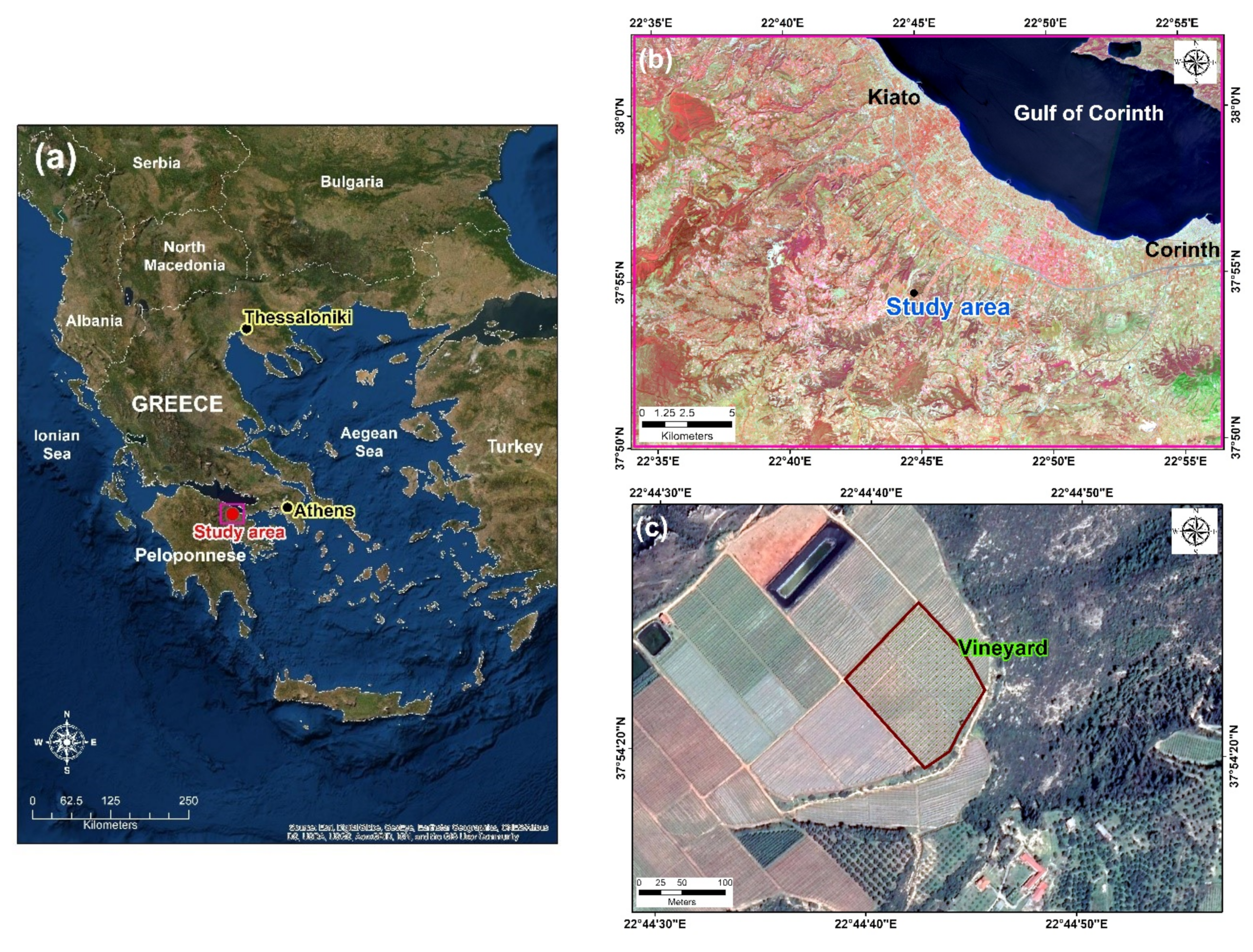
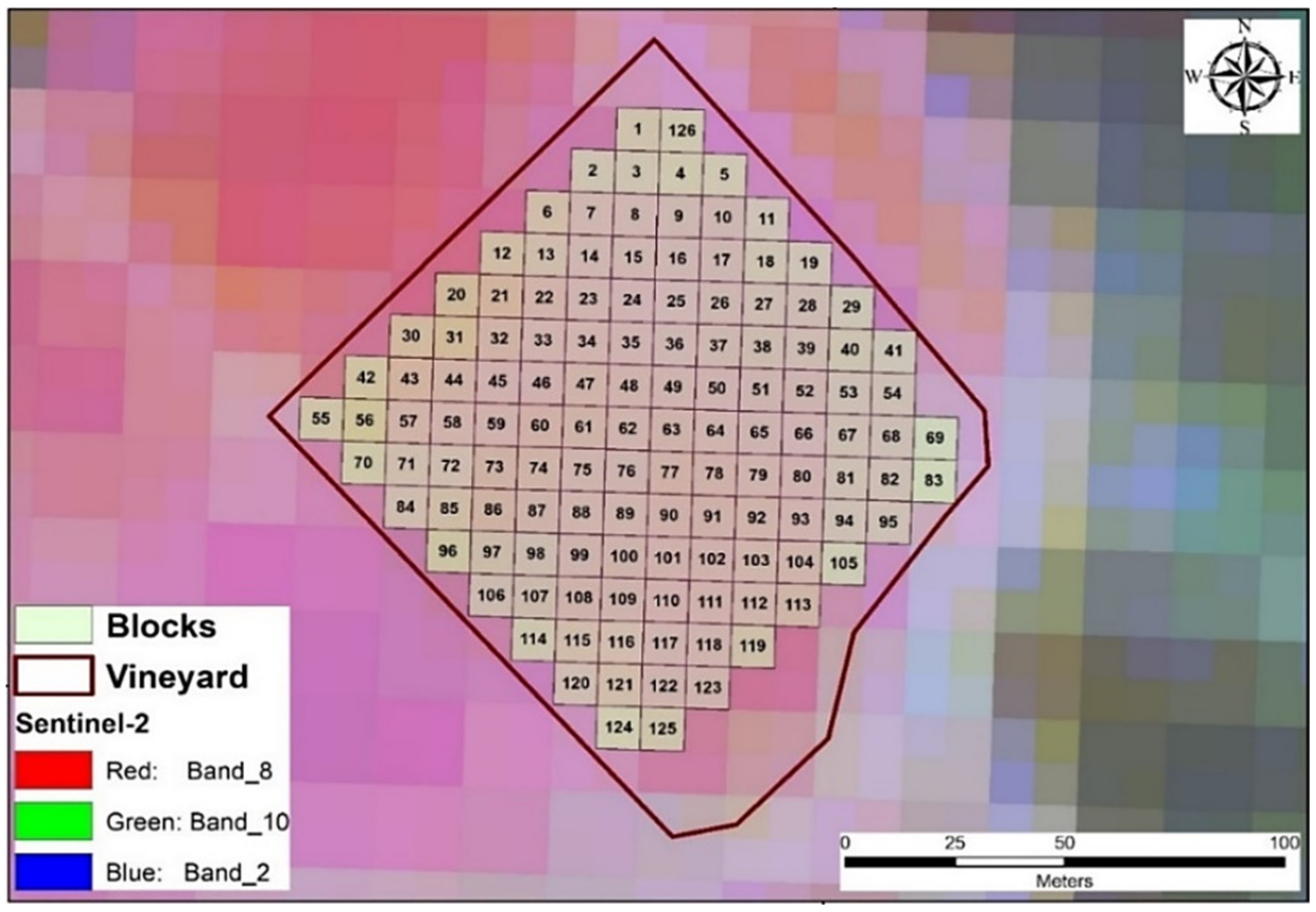
2.1. Study Area
2.2. Datasets and Methodology
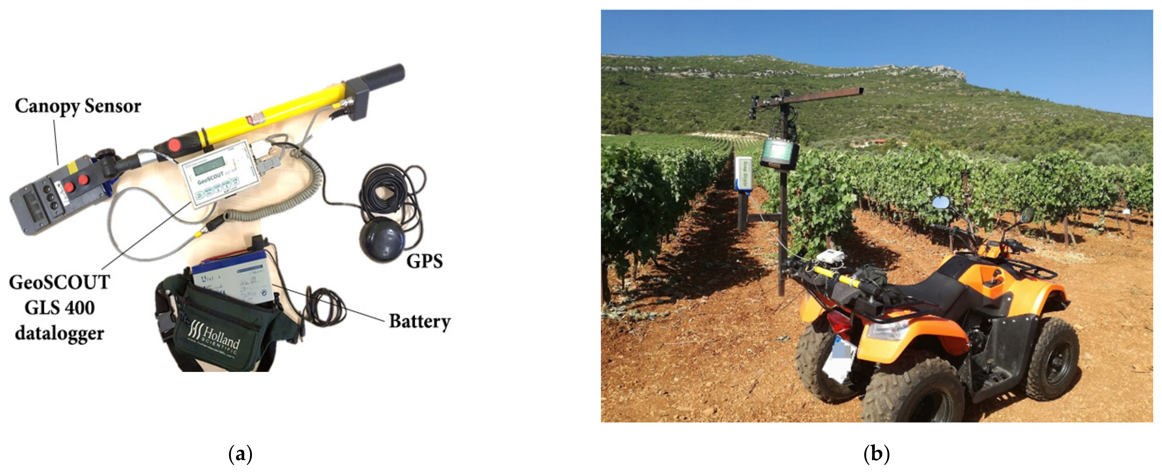
2.2.1. Proximal and Remote-Sensing Data
2.2.2. Spectral Characteristics of Vegetation Indices and Vegetation Biophysical Variables
2.2.3. Yield Estimation and Statistical Analysis
2.2.4. Processing and Statistical Analysis Software
3. Results
3.1. Descriptive Statistics
3.2. Satellite and Proximal Based NDVI and NDRE Comparison
3.3. Vegetation Indices and Yield Measurements
4. Discussion
4.1. Proximal- and Remote-Sensing Multi-Seasonal Comparison
4.2. VIs–VBVs and Yield Correlation
5. Conclusions
Author Contributions
Funding
Institutional Review Board Statement
Informed Consent Statement
Data Availability Statement
Acknowledgments
Conflicts of Interest
References
- Cunha, M.; Marçal, A.R.S.; Silva, L. Very early prediction of wine yield based on satellite data from Vegetation. Int. J. Remote Sens. 2010, 31, 3125–3142. [Google Scholar] [CrossRef]
- Matese, A.; Di Gennaro, S.F. Technology in precision viticulture: A state of the art review. Int. J. Wine Res. 2015, 7, 69. [Google Scholar] [CrossRef] [Green Version]
- Hall, A.; Lamb, D.W.; Holzapfel, B.; Louis, J. Optical remote sensing applications in viticulture—A review. Aust. J. Grape Wine Res. 2002, 8, 36–47. [Google Scholar] [CrossRef]
- Belmonte, A.C.; Jochum, A.M.; García, A.C.; Rodríguez, A.M.; Fuster, P.L. Irrigation management from space: Towards user-friendly products. Irrig. Drain. Syst. 2005, 19, 337–353. [Google Scholar] [CrossRef]
- Anastasiou, E.; Tsiropoulos, Z.; Balafoutis, T.; Fountas, S.; Templalexis, C.; Lentzou, D.; Xanthopoulos, G. Spatiotemporal stability of management zones in a table grapes vineyard in Greece. Adv. Anim. Biosci. 2017, 8, 510–514. [Google Scholar] [CrossRef]
- Arnó, J.; Martínez-Casasnovas, J.A.; Ribes-Dasi, M.; Rosell, J.R. Review. Precision Viticulture. Research topics, challenges and opportunities in site-specific vineyard management. Span. J. Agric. Res. 2009, 7, 779–790. [Google Scholar] [CrossRef] [Green Version]
- Campos, I.; González-Gómez, L.; Villodre, J.; Calera, M.; Campoy, J.; Jiménez, N.; Plaza, C.; Sánchez-Prieto, S.; Calera, A. Mapping within-field variability in wheat yield and biomass using remote sensing vegetation indices. Precis. Agric. 2019, 20, 214–236. [Google Scholar] [CrossRef]
- Pallottino, F.; Biocca, M.; Nardi, P.; Figorilli, S.; Menesatti, P.; Costa, C. Science mapping approach to analyze the research evolution on precision agriculture: World, EU and Italian situation. Precis. Agric. 2018, 19, 1011–1026. [Google Scholar] [CrossRef]
- Khaliq, A.; Comba, L.; Biglia, A.; Ricauda Aimonino, D.; Chiaberge, M.; Gay, P. Comparison of Satellite and UAV-Based Multispectral Imagery for Vineyard Variability Assessment. Remote Sens. 2019, 11, 436. [Google Scholar] [CrossRef] [Green Version]
- Di Gennaro, S.F.; Matese, A.; Gioli, B.; Toscano, P.; Zaldei, A.; Palliotti, A.; Genesio, L. Multisensor approach to assess vineyard thermal dynamics combining high-resolution unmanned aerial vehicle (UAV) remote sensing and wireless sensor network (WSN) proximal sensing. Sci. Hortic. (Amst.) 2017, 221, 83–87. [Google Scholar] [CrossRef]
- Kavvadias, A.; Psomiadis, E.; Chanioti, M.; Tsitouras, A.; Toulios, L.; Dercas, N. Unmanned Aerial Vehicle (UAV) data analysis for fertilization dose assessment. In Proceedings of the SPIE—The International Society for Optical Engineering, Warsaw, Poland, 2 November 2017; Volume 10421. [Google Scholar]
- Hall, A.; Wilson, M.A. Object-based analysis of grapevine canopy relationships with winegrape composition and yield in two contrasting vineyards using multitemporal high spatial resolution optical remote sensing. Int. J. Remote Sens. 2013, 34, 1772–1797. [Google Scholar] [CrossRef]
- Psomiadis, E.; Dercas, N.; Dalezios, N.R.; Spiropoulos, N. Evaluation and cross-comparison of vegetation indices for crop monitoring from sentinel-2 and worldview-2 images. In Proceedings of the Remote Sensing for Agriculture, Ecosystems, and Hydrology XIX, Warsaw, Poland, 12–14 September 2017; Neale, C.M., Maltese, A., Eds.; SPIE-International Society for Optics and Photonics: Warsaw, Poland, 2017; Volume 10421, p. 79. [Google Scholar]
- Fountas, S.; Espejo-Garcia, B.; Kasimati, A.; Mylonas, N.; Darra, N. The Future of Digital Agriculture: Technologies and Opportunities. IT Prof. 2020, 22, 24–28. [Google Scholar] [CrossRef]
- Fountas, S.; Aggelopoulou, K.; Bouloulis, C.; Nanos, G.D.; Wulfsohn, D.; Gemtos, T.A.; Paraskevopoulos, A.; Galanis, M. Site-specific management in an olive tree plantation. Precis. Agric. 2011, 12, 179–195. [Google Scholar] [CrossRef]
- De Benedetto, D.; Castrignano, A.; Diacono, M.; Rinaldi, M.; Ruggieri, S.; Tamborrino, R. Field partition by proximal and remote sensing data fusion. Biosyst. Eng. 2013, 114, 372–383. [Google Scholar] [CrossRef]
- Mulla, D.J. Twenty five years of remote sensing in precision agriculture: Key advances and remaining knowledge gaps. Biosyst. Eng. 2013, 114, 358–371. [Google Scholar] [CrossRef]
- Lamb, D.W.; Weedon, M.M.; Bramley, R.G.V. Using remote sensing to predict grape phenolics and colour at harvest in a Cabernet Sauvignon vineyard: Timing observations against vine phenology and optimising image resolution. Aust. J. Grape Wine Res. 2008, 10, 46–54. [Google Scholar] [CrossRef] [Green Version]
- Meggio, F.; Zarco-Tejada, P.J.; Núñez, L.C.; Sepulcre-Cantó, G.; González, M.R.; Martín, P. Grape quality assessment in vineyards affected by iron deficiency chlorosis using narrow-band physiological remote sensing indices. Remote Sens. Environ. 2010, 114, 1968–1986. [Google Scholar] [CrossRef] [Green Version]
- Mouazen, A.M.; Alexandridis, T.; Buddenbaum, H.; Cohen, Y.; Moshou, D.; Mulla, D.; Nawar, S.; Sudduth, K.A. Monitoring. In Agricultural Internet of Things and Decision Support for Precision Smart Farming; Elsevier Inc.: Amsterdam, The Netherlands, 2020; pp. 35–138. ISBN 9780128183731. [Google Scholar]
- Chatziantoniou, A.; Petropoulos, G.P.; Psomiadis, E. Co-Orbital Sentinel 1 and 2 for LULC mapping with emphasis on wetlands in a mediterranean setting based on machine learning. Remote Sens. 2017, 9, 1259. [Google Scholar] [CrossRef] [Green Version]
- Psomiadis, E.; Soulis, K.X.; Efthimiou, N. Using SCS-CN and earth observation for the comparative assessment of the hydrological effect of gradual and abrupt spatiotemporal land cover changes. Water 2020, 12, 1386. [Google Scholar] [CrossRef]
- Belgiu, M.; Csillik, O. Sentinel-2 cropland mapping using pixel-based and object-based time-weighted dynamic time warping analysis. Remote Sens. Environ. 2018, 204, 509–523. [Google Scholar] [CrossRef]
- Di Gennaro, S.; Dainelli, R.; Palliotti, A.; Toscano, P.; Matese, A. Sentinel-2 Validation for Spatial Variability Assessment in Overhead Trellis System Viticulture Versus UAV and Agronomic Data. Remote Sens. 2019, 11, 2573. [Google Scholar] [CrossRef] [Green Version]
- Esch, T.; Metz, A.; Marconcini, M.; Keil, M. Combined use of multi-seasonal high and medium resolution satellite imagery for parcel-related mapping of cropland and grassland. Int. J. Appl. Earth Obs. Geoinf. 2014, 28, 230–237. [Google Scholar] [CrossRef]
- Löw, F.; Michel, U.; Dech, S.; Conrad, C. Impact of feature selection on the accuracy and spatial uncertainty of per-field crop classification using Support Vector Machines. ISPRS J. Photogramm. Remote Sens. 2013, 85, 102–119. [Google Scholar] [CrossRef]
- Fountas, S.; Anastasiou, E.; Balafoutis, A.; Koundouras, S.; Theoharis, S.; Theodorou, N. The influence of vine variety and vineyard management on the effectiveness of canopy sensors to predict winegrape yield and quality. In Proceedings of the International Conference of Agricultural Engineering, Zurich, Switzerland, 6–10 July 2014; p. 8. [Google Scholar]
- Lamb, D.W.; Trotter, M.G.; Schneider, D.A. Ultra low-level airborne (ULLA) sensing of crop canopy reflectance: A case study using a CropCircleTM sensor. Comput. Electron. Agric. 2009, 69, 86–91. [Google Scholar] [CrossRef]
- Anastasiou, E.; Castrignanò, A.; Arvanitis, K.; Fountas, S. A multi-source data fusion approach to assess spatial-temporal variability and delineate homogeneous zones: A use case in a table grape vineyard in Greece. Sci. Total Environ. 2019, 684, 155–163. [Google Scholar] [CrossRef] [PubMed]
- Cao, Q.; Miao, Y.; Feng, G.; Gao, X.; Li, F.; Liu, B.; Yue, S.; Cheng, S.; Ustin, S.L.; Khosla, R. Active canopy sensing of winter wheat nitrogen status: An evaluation of two sensor systems. Comput. Electron. Agric. 2015, 112, 54–67. [Google Scholar] [CrossRef]
- Stamatiadis, S.; Taskos, D.; Tsadila, E.; Christofides, C.; Tsadilas, C.; Schepers, J.S. Comparison of passive and active canopy sensors for the estimation of vine biomass production. Precis. Agric. 2010, 11, 306–315. [Google Scholar] [CrossRef] [Green Version]
- Bramley, R.G.V.; Trought, M.C.T.; Praat, J.-P. Vineyard variability in Marlborough, New Zealand: Characterising variation in vineyard performance and options for the implementation of Precision Viticulture. Aust. J. Grape Wine Res. 2011, 17, 72–78. [Google Scholar] [CrossRef]
- Taskos, D.G.; Koundouras, S.; Stamatiadis, S.; Zioziou, E.; Nikolaou, N.; Karakioulakis, K.; Theodorou, N. Using active canopy sensors and chlorophyll meters to estimate grapevine nitrogen status and productivity. Precis. Agric. 2014, 16, 77–98. [Google Scholar] [CrossRef]
- Yao, Y.; Miao, Y.; Jiang, R.; Khosla, R.; Gnyp, M.L.; Bareth, G. Evaluating different active crop canopy sensors for estimating rice yield potential. In Proceedings of the 2013 2nd International Conference on Agro-Geoinformatics: Information for Sustainable Agriculture, Agro-Geoinformatics 2013, Fairfax, VI, USA, 12–16 August 2013; pp. 538–542. [Google Scholar]
- Li, F.; Miao, Y.; Feng, G.; Yuan, F.; Yue, S.; Gao, X.; Liu, Y.; Liu, B.; Ustin, S.L.; Chen, X. Improving estimation of summer maize nitrogen status with red edge-based spectral vegetation indices. Field Crop. Res. 2014, 157, 111–123. [Google Scholar] [CrossRef]
- Cao, Q.; Miao, Y.; Li, F.; Gao, X.; Liu, B.; Lu, D.; Chen, X. Developing a new Crop Circle active canopy sensor-based precision nitrogen management strategy for winter wheat in North China Plain. Precis. Agric. 2017, 18, 2–18. [Google Scholar] [CrossRef]
- Matese, A.; Di Gennaro, S.F.; Miranda, C.; Berton, A.; Santesteban, L.G. Evaluation of spectral-based and canopy-based vegetation indices from UAV and Sentinel 2 images to assess spatial variability and ground vine parameters. Adv. Anim. Biosci. 2017, 8, 817–822. [Google Scholar] [CrossRef]
- Anastasiou, E.; Balafoutis, A.; Darra, N.; Psiroukis, V.; Biniari, A.; Xanthopoulos, G.; Fountas, S. Satellite and Proximal Sensing to Estimate the Yield and Quality of Table Grapes. Agriculture 2018, 8, 94. [Google Scholar] [CrossRef] [Green Version]
- Kavvadias, A.; Psomiadis, E.; Chanioti, M.; Gala, E.; Michas, S. Precision agriculture—Comparison and evaluation of innovative very high resolution (UAV) and LandSat data. In Proceedings of the CEUR Workshop Proceedings, Brussels, Belgium, 27 March 2015; Volume 1498. [Google Scholar]
- Bellvert, J.; Zarco-Tejada, P.J.; Marsal, J.; Girona, J.; González-Dugo, V.; Fereres, E. Vineyard irrigation scheduling based on airborne thermal imagery and water potential thresholds. Aust. J. Grape Wine Res. 2016, 22, 307–315. [Google Scholar] [CrossRef] [Green Version]
- Hall, A.; Louis, J.P.; Lamb, D.W. Low-resolution remotely sensed images of winegrape vineyards map spatial variability in planimetric canopy area instead of leaf area index. Aust. J. Grape Wine Res. 2008, 14, 9–17. [Google Scholar] [CrossRef]
- Xue, J.; Su, B. Significant remote sensing vegetation indices: A review of developments and applications. J. Sens. 2017, 2017, 1353691. [Google Scholar] [CrossRef] [Green Version]
- Rouse, J.W.; Haas, R.H.; Schell, J.A.; Deering, W.D. Monitoring vegetation systems in the Great Plains with ERTS. In Proceedings of the Third Earth Resources Technology Satellite–1 Symposium, Washington, DC, USA, 10–14 December 1973; Freden, S.C., Mercanti, E.P., Becker, M., Eds.; NASA: Washington, DC, USA, 1974; pp. 309–317. [Google Scholar]
- Hatfield, J.L.; Gitelson, A.A.; Schepers, J.S.; Walthall, C.L. Application of spectral remote sensing for agronomic decisions. Agron. J. 2008, 100, S-117–S-131. [Google Scholar] [CrossRef] [Green Version]
- Magarreiro, C.; Gouveia, C.; Barroso, C.; Trigo, I. Modelling of Wine Production Using Land Surface Temperature and FAPAR—The Case of the Douro Wine Region. Remote Sens. 2019, 11, 604. [Google Scholar] [CrossRef] [Green Version]
- Borgogno-Mondino, E.; de Palma, L.; Novello, V. Investigating Sentinel 2 Multispectral Imagery Efficiency in Describing Spectral Response of Vineyards Covered with Plastic Sheets. Agronomy 2020, 10, 1909. [Google Scholar] [CrossRef]
- Stroppiana, D.; Pepe, M.; Boschetti, M.; Crema, A.; Candiani, G.; Giordan, D.; Baldo, M.; Allasia, P.; Monopoli, L. Estimating Crop Density From Multi-Spectral Uav Imagery in Maize Crop. Int. Arch. Photogramm. Remote Sens. Spat. Inf. Sci. 2019, XLII-2/W13, 619–624. [Google Scholar] [CrossRef] [Green Version]
- Morlin Carneiro, F.; Angeli Furlani, C.E.; Zerbato, C.; Candida de Menezes, P.; da Silva Gírio, L.A.; Freire de Oliveira, M. Comparison between vegetation indices for detecting spatial and temporal variabilities in soybean crop using canopy sensors. Precis. Agric. 2020, 21, 979–1007. [Google Scholar] [CrossRef]
- Peloponnese Wine Region, Greece|Winetourism. Available online: https://www.winetourism.com/wine-region/peloponnese/ (accessed on 24 March 2021).
- Dobrowski, S.Z.; Ustin, S.; Wolpert, J.A. Remote estimation of vine canopy density in vertically shoot-positioned vineyards: Determining optimal vegetation indices. Aust. J. Grape Wine Res. 2002, 8, 117–125. [Google Scholar] [CrossRef]
- Ballesteros, R.; Intrigliolo, D.S.; Ortega, J.F.; Ramírez-Cuesta, J.M.; Buesa, I.; Moreno, M.A. Vineyard yield estimation by combining remote sensing, computer vision and artificial neural network techniques. Precis. Agric. 2020, 21, 1242–1262. [Google Scholar] [CrossRef]
- Kottek, M.; Grieser, J.; Beck, C.; Rudolf, B.; Rubel, F. World map of the Köppen-Geiger climate classification updated. Meteorol. Z. 2006, 15, 259–263. [Google Scholar] [CrossRef]
- Psomiadis, E.; Diakakis, M.; Soulis, K.X. Combining SAR and Optical Earth Observation with Hydraulic Simulation for Flood Mapping and Impact Assessment. Remote Sens. 2020, 12, 3980. [Google Scholar] [CrossRef]
- Taylor, J.; Tisseyre, B.; Praat, J.-P. Information and Technology for Sustainable Fruit and Vegetable Production Bottling Good Information: Mixing Tradition and Technology in vineyards. In Proceedings of the Information and Technology for Sustainable Fruit and Vegetable Production, Montpellier, France, 12–16 September 2005; pp. 719–736. [Google Scholar]
- Bonilla, I.; Martínez, D.; Toda, F.; Martínez-Casasnovas, J.A. Grape quality assessment by airborne remote sensing over three years. Precis. Agric. 2013, 611–615. [Google Scholar] [CrossRef]
- Kazmierski, M.; Glemas, P.; Rousseau, J.; Tisseyre, B. Temporal stability of within-field patterns of ndvi in non irrigated mediterranean vineyards. J. Int. Sci. Vigne Vin. 2011, 45, 61–73. [Google Scholar] [CrossRef]
- Sozzi, M.; Kayad, A.; Marinello, F.; Taylor, J.; Tisseyre, B. Comparing vineyard imagery acquired from Sentinel-2 and Unmanned Aerial Vehicle (UAV) platform. OENO One 2020, 54, 189–197. [Google Scholar] [CrossRef] [Green Version]
- Piragnolo, M.; Lusiani, G.; Pirotti, F. Comparison of Vegetation Indices from RPAS and Sentinel-2 Imagery for Detecting Permanent Pastures. ISPRS Int. Arch. Photogramm. Remote Sens. Spat. Inf. Sci. 2018, XLII-3, 1381–1387. [Google Scholar] [CrossRef] [Green Version]
- Tagarakis, A.; Liakos, V.; Fountas, S.; Koundouras, S.; Gemtos, T.A. Management zones delineation using fuzzy clustering techniques in grapevines. Precis. Agric. 2013, 14, 18–39. [Google Scholar] [CrossRef]
- Efthimiou, N.; Psomiadis, E.; Panagos, P. Fire severity and soil erosion susceptibility mapping using multi-temporal Earth Observation data: The case of Mati fatal wildfire in Eastern Attica, Greece. Catena 2020, 187, 104320. [Google Scholar] [CrossRef]
- Barnes, E.M.; Clarke, T.R.; Richards, S.E.; Colaizzi, P.D.; Haberland, J.; Kostrzewski, M.; Waller, P.; Choi, C.; Riley, E.; Thompson, T. Coincident detection of crop water stress, nitrogen status and canopy density using ground-based multispectral data. In Proceedings of the Fifth International Conference on Precision Agriculture and Other Resource Management, Bloom, MN, USA, 16–19 July 2000. [Google Scholar]
- Lu, J.; Miao, Y.; Shi, W.; Li, J.; Yuan, F. Evaluating different approaches to non-destructive nitrogen status diagnosis of rice using portable RapidSCAN active canopy sensor. Sci. Rep. 2017, 7, 14073. [Google Scholar] [CrossRef]
- Bonfil, D.J. Wheat phenomics in the field by RapidScan: NDVI vs. NDRE. Isr. J. Plant Sci. 2017, 64, 41–54. [Google Scholar] [CrossRef]
- Qi, J.; Chehbouni, A.; Huete, A.R.; Kerr, Y.H.; Sorooshian, S. A modified soil adjusted vegetation index. Remote Sens. Environ. 1994, 48, 119–126. [Google Scholar] [CrossRef]
- Gao, B.C. NDWI—A normalized difference water index for remote sensing of vegetation liquid water from space. Remote Sens. Environ. 1996, 58, 257–266. [Google Scholar] [CrossRef]
- Gitelson, A.A.; Kaufman, Y.J.; Stark, R.; Rundquist, D. Novel algorithms for remote estimation of vegetation fraction. Remote Sens. Environ. 2002, 80, 76–87. [Google Scholar] [CrossRef] [Green Version]
- Carlson, T.N.; Gillies, R.R.; Perry, E.M. A method to make use of thermal infrared temperature and NDVI measurements to infer surface soil water content and fractional vegetation cover. Remote Sens. Rev. 1994, 9, 161–173. [Google Scholar] [CrossRef]
- Pickett-Heaps, C.A.; Canadell, J.G.; Briggs, P.R.; Gobron, N.; Haverd, V.; Paget, M.J.; Pinty, B.; Raupach, M.R. Evaluation of six satellite-derived Fraction of Absorbed Photosynthetic Active Radiation (FAPAR) products across the Australian continent. Remote Sens. Environ. 2014, 140, 241–256. [Google Scholar] [CrossRef]
- Qin, J.; Zhao, L.; Chen, Y.; Yang, K.; Yang, Y.; Chen, Z.; Lu, H. Inter-comparison of spatial upscaling methods for evaluation of satellite-based soil moisture. J. Hydrol. 2015, 523, 170–178. [Google Scholar] [CrossRef]
- Minasny, B.; McBratney, A.B.; Whelan, B.M. VESPER Version 1.6; Sydney University Press: Sydney, Austalia, 2005. [Google Scholar]
- Fiorillo, E.; Crisci, A.; De Filippis, T.; Di Gennaro, S.F.; Di Blasi, S.; Matese, A.; Primicerio, J.; Vaccari, F.P.; Genesio, L. Airborne high-resolution images for grape classification: Changes in correlation between technological and late maturity in a Sangiovese vineyard in Central Italy. Aust. J. Grape Wine Res. 2012, 18, 80–90. [Google Scholar] [CrossRef]
- Taylor, J.A.; Bates, T.R. A discussion on the significance associated with Pearson’s correlation in precision agriculture studies. Precis. Agric. 2013, 14, 558–564. [Google Scholar] [CrossRef]
- STATGRAPHICS Version 16. Available online: http://www.statvision.com/version16.htm (accessed on 21 December 2020).
- Ayalew, L.; Yamagishi, H. The application of GIS-based logistic regression for landslide susceptibility mapping in the Kakuda-Yahiko Mountains, Central Japan. Geomorphology 2005, 65, 15–31. [Google Scholar] [CrossRef]
- Youssef, A.M.; Al-Kathery, M.; Pradhan, B. Landslide susceptibility mapping at Al-Hasher area, Jizan (Saudi Arabia) using GIS-based frequency ratio and index of entropy models. Geosci. J. 2015, 19, 113–134. [Google Scholar] [CrossRef]
- Akgun, A.; Sezer, E.A.; Nefeslioglu, H.A.; Gokceoglu, C.; Pradhan, B. An easy-to-use MATLAB program (MamLand) for the assessment of landslide susceptibility using a Mamdani fuzzy algorithm. Comput. Geosci. 2012, 38, 23–34. [Google Scholar] [CrossRef]
- Gatti, M.; Squeri, C.; Kleshcheva, E.; Garavani, A.; Vincini, M.; Poni, S. Studying spatial and temporal variability of a “Barbera” vineyard with traditional and precision approaches. Acta Hortic. 2020, 1279, 247–254. [Google Scholar] [CrossRef]
- Reynolds, A.G.; Lee, H.-S.; Dorin, B.; Brown, R.; Jollineau, M.; Shemrock, A.; Crombleholme, M.; Jobin Poirier, E.; Zheng, W.; Gasnier, M.; et al. Mapping Cabernet Franc vineyards by unmanned aerial vehicles (UAVs) for variability in vegetation indices, water status, and virus titer. E3S Web Conf. 2018, 50, 02010. [Google Scholar] [CrossRef]
- Primicerio, J.; Di Gennaro, S.F.; Fiorillo, E.; Genesio, L.; Lugato, E.; Matese, A.; Vaccari, F.P. A flexible unmanned aerial vehicle for precision agriculture. Precis. Agric. 2012, 13, 517–523. [Google Scholar] [CrossRef]
- Henry, D.; Aubert, H.; Veronese, T. Proximal Radar Sensors for Precision Viticulture. IEEE Trans. Geosci. Remote Sens. 2019, 57, 4624–4635. [Google Scholar] [CrossRef]
- Stamatiadis, S.; Taskos, D.; Tsadilas, C.; Christofides, C.; Tsadila, E.; Schepers, J.S. Relation of Ground-Sensor Canopy Reflectance to Biomass Production and Grape Color in Two Merlot Vineyards. Am. J. Enol. Vitic. 2006, 57, 415–422. [Google Scholar]
- Martínez-Beltrán, C.; Jochum, M.A.O.; Calera, A.; Meliá, J. Multisensor comparison of NDVI for a semi-arid environment in Spain. Int. J. Remote Sens. 2009, 30, 1355–1384. [Google Scholar] [CrossRef]
- Mathews, A.J. Object-based spatiotemporal analysis of vine canopy vigor using an inexpensive unmanned aerial vehicle remote sensing system. J. Appl. Remote Sens. 2014, 8, 085199. [Google Scholar] [CrossRef]
- Acevedo-Opazo, C.; Tisseyre, B.; Guillaume, S.; Ojeda, H. The potential of high spatial resolution information to define within-vineyard zones related to vine water status. Precis. Agric. 2008, 9, 285–302. [Google Scholar] [CrossRef] [Green Version]
- Sun, L.; Gao, F.; Anderson, M.; Kustas, W.; Alsina, M.; Sanchez, L.; Sams, B.; McKee, L.; Dulaney, W.; White, W.; et al. Daily Mapping of 30 m LAI and NDVI for Grape Yield Prediction in California Vineyards. Remote Sens. 2017, 9, 317. [Google Scholar] [CrossRef] [Green Version]
- Johnson, L.F. Temporal stability of an NDVI-LAI relationship in a Napa Valley vineyard. Aust. J. Grape Wine Res. 2003, 9, 96–101. [Google Scholar] [CrossRef]
- Kotsaki, E.; Reynolds, A.G.; Brown, R.; Jollineau, M.; Lee, H.S.; Aubie, E. Proximal sensing and relationships to soil and vine water status, yield, and berry composition in ontario vineyards. Am. J. Enol. Vitic. 2020, 71, 114–131. [Google Scholar] [CrossRef]
- Costa, B.R.S.; Oldoni, H.; Rocha, R.C.; Bassoi, L.H. Delimitation of homogeneous zones in vineyards using geostatistics and multivariate analysis of different vegetation indices. Eng. Agric. 2019, 39, 13–22. [Google Scholar] [CrossRef]
- Matese, A.; Toscano, P.; Di Gennaro, S.; Genesio, L.; Vaccari, F.; Primicerio, J.; Belli, C.; Zaldei, A.; Bianconi, R.; Gioli, B. Intercomparison of UAV, Aircraft and Satellite Remote Sensing Platforms for Precision Viticulture. Remote Sens. 2015, 7, 2971–2990. [Google Scholar] [CrossRef] [Green Version]
- Erena, M.; Montesinos, S.; Portillo, D.; Alvarez, J.; Marin, C.; Fernandez, L.; Henarejos, J.M.; Ruiz, L.A. Configuration and Specifications of an Unmanned Aerial Vehicle for Precision Agriculture. In Proceedings of the International Archives of the Photogrammetry, Remote Sensing and Spatial Information Sciences—XXIII ISPRS Congress, Prague, Chech Republic, 12–19 July 2016; pp. 809–816. [Google Scholar]
- Spachos, P.; Gregori, S. Integration of Wireless Sensor Networks and Smart UAVs for Precision Viticulture. IEEE Internet Comput. 2019, 23, 8–16. [Google Scholar] [CrossRef]
- García-Estévez, I.; Quijada-Morín, N.; Rivas-Gonzalo, J.C.; Martínez-Fernández, J.; Sánchez, N.; Herrero-Jiménez, C.M.; Escribano-Bailón, M.T. Relationship between hyperspectral indices, agronomic parameters and phenolic composition of Vitis vinifera cv Tempranillo grapes. J. Sci. Food Agric. 2017, 97, 4066–4074. [Google Scholar] [CrossRef] [Green Version]


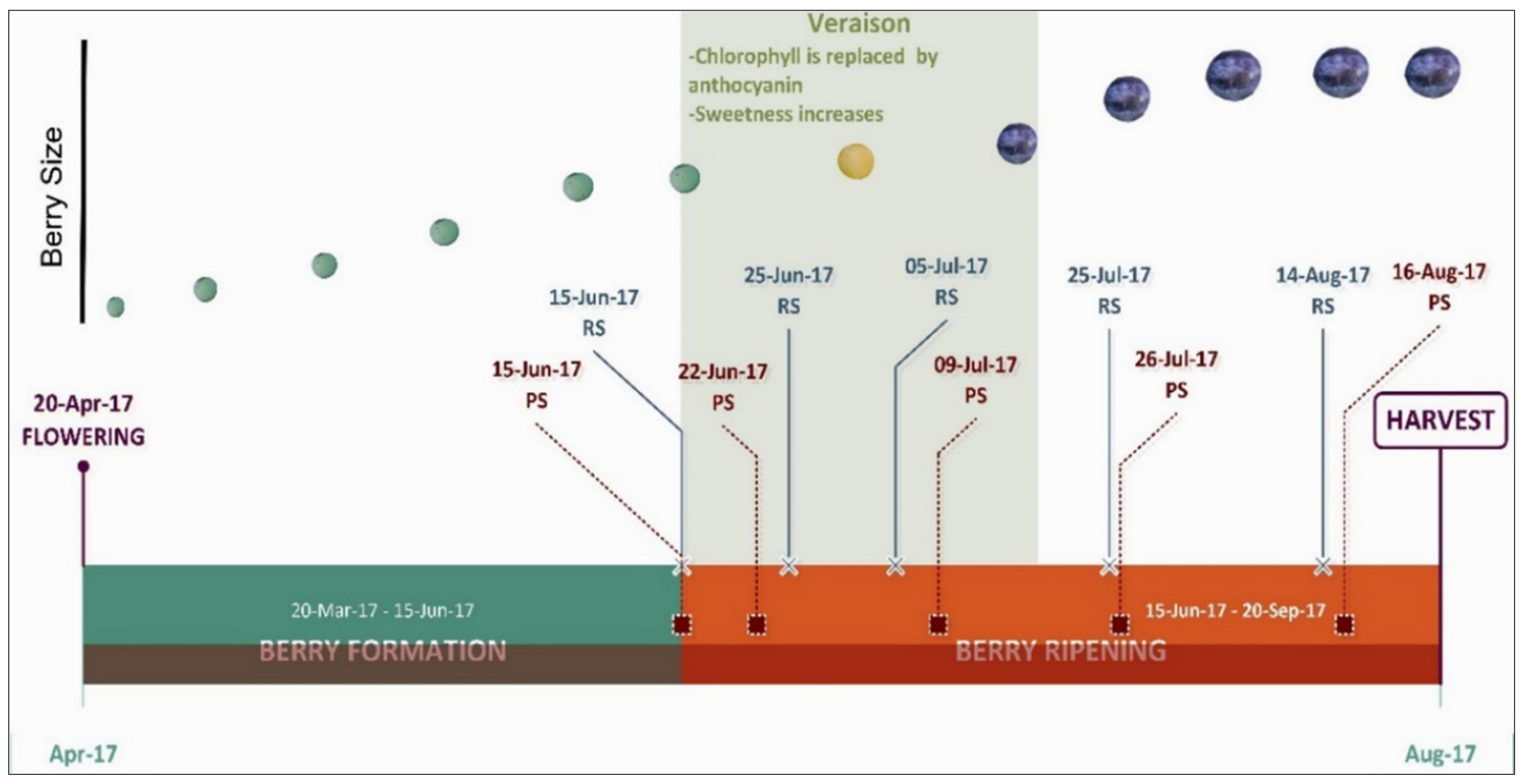
| Growth Stages | Proximal-Sensing Dates | Satellite-Sensing Dates |
|---|---|---|
| SV | 15 June 2017 | 15 June 2017 |
| MV-1 | 22 June 2017 | 25 June 2017 |
| MV-2 | 09 July 2017 | 05 July 2017 |
| H-1 | 26 July 2017 | 25 July 2017 |
| H-2 | 16 August 2017 | 14 August 2017 |
| Sensor–VI–Growing Stage | Mean | Min | Max | SD | CV (%) |
|---|---|---|---|---|---|
| SV: CCNDVI/SNDVI | 0.66/0.61 | 0.61/0.39 | 0.71/0.69 | 0.02/0.05 | 3.23/8.31 |
| MV-1: CCNDVI/SNDVI | 0.60/0.62 | 0.57/0.41 | 0.63/0.71 | 0.01/0.05 | 2.15/8.67 |
| MV-2: CCNDVI/SNDVI | 0.65/0.63 | 0.60/0.34 | 0.67/0.71 | 0.02/0.06 | 2.53 |
| H-1: CCNDVI/SNDVI | 0.64/0.67 | 0.61/0.33 | 0.67/0.75 | 0.01/0.07 | 1.60/10.75 |
| H-2: CCNDVI/SNDVI | 0.61/0.74 | 0.54/0.41 | 0.64/0.84 | 0.02/0.08 | 3.03/10.31 |
| SV: CCNDRE/SNDRE | 0.53/0.42 | 0.50/0.24 | 0.55/0.46 | 0.01/0.03 | 1.93/8.31 |
| MV-1: CCNDRE/SNDRE | 0.44/0.46 | 0.22/0.32 | 0.62/0.52 | 0.09/0.04 | 19.71/8.00 |
| MV-2: CCNDRE/SNDRE | 0.36/0.45 | 0.32/0.32 | 0.40/0.50 | 0.02/0.04 | 4.65/8.61 |
| H-1: CCNDRE/SNDRE | 0.51/0.48 | 0.34/0.30 | 0.63/0.54 | 0.06/0.05 | 11.23/10.81 |
| H-2: CCNDRE/SNDRE | 0.45/0.53 | 0.30/0.25 | 0.64/0.60 | 0.10/0.06 | 21.39/11.80 |
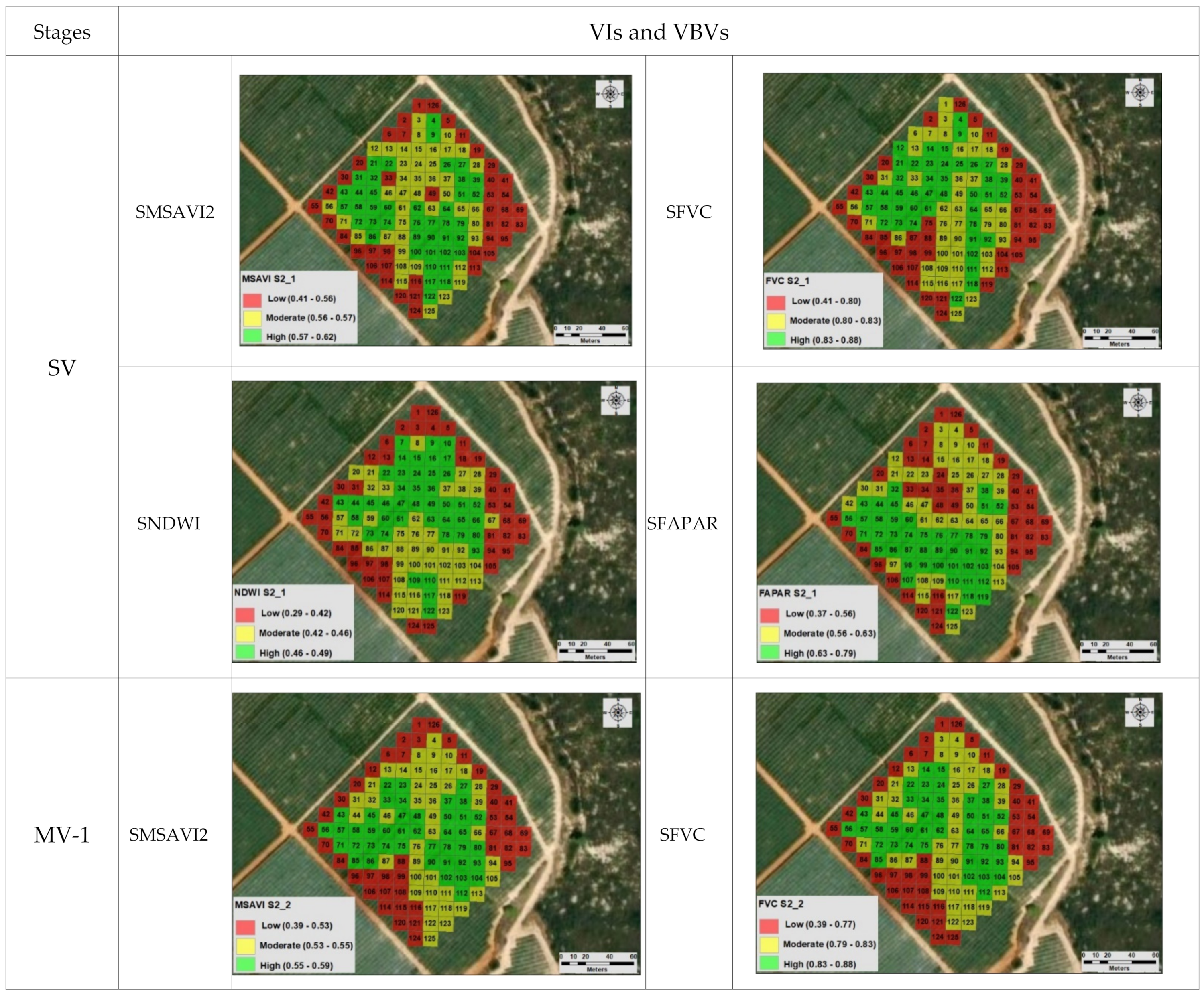
| SV: SMSAVI2 | 0.55 | 0.41 | 0.62 | 0.04 | 6.85 |
| MV-1: SMSAVI2 | 0.53 | 0.39 | 0.59 | 0.04 | 6.60 |
| MV-2: SMSAVI2 | 0.52 | 0.34 | 0.57 | 0.04 | 7.50 |
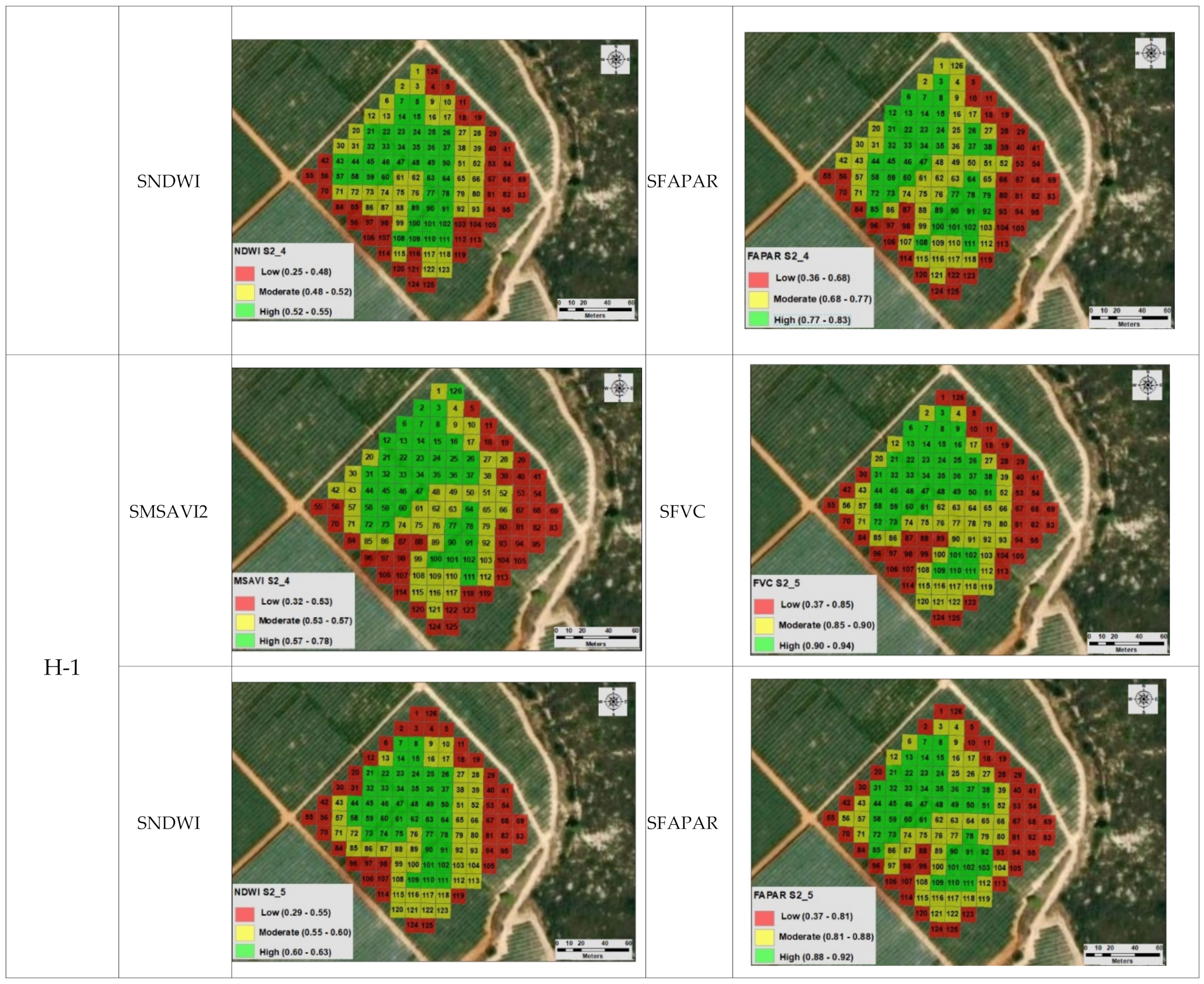
| H-1: SMSAVI2 | 0.54 | 0.32 | 0.78 | 0.06 | 10.99 |
| H-2: SMSAVI2 | 0.60 | 0.37 | 0.70 | 0.06 | 10.43 |
| SV: SNDWI | 0.44 | 0.29 | 0.49 | 0.04 | 8.62 |
| MV-1: SNDWI | 0.44 | 0.29 | 0.49 | 0.04 | 8.74 |
| MV-2: SNDWI | 0.47 | 0.28 | 0.52 | 0.05 | 10.48 |
| H-1: SNDWI | 0.49 | 0.25 | 0.55 | 0.06 | 11.87 |
| H-2: SNDWI | 0.55 | 0.29 | 0.63 | 0.07 | 12.02 |
| SV: SFVC | 0.79 | 0.41 | 0.88 | 0.08 | 10.59 |
| MV-1: SFVC | 0.79 | 0.39 | 0.88 | 0.08 | 10.38 |
| MV-2: S FVC | 0.75 | 0.28 | 0.83 | 0.09 | 12.12 |
| H-1: S FVC | 0.77 | 0.29 | 0.87 | 0.11 | 14.59 |
| H-2: S FVC | 0.85 | 0.37 | 0.94 | 0.10 | 11.89 |
| SV: SFAPAR | 0.59 | 0.37 | 0.79 | 0.09 | 15.13 |
| MV-1: SFAPAR | 0.61 | 0.37 | 0.80 | 0.10 | 15.78 |
| MV-2: SFAPAR | 0.62 | 0.36 | 0.76 | 0.09 | 14.56 |
| H-1: SFAPAR | 0.70 | 0.36 | 0.83 | 0.12 | 16.57 |
| H-2: SFAPAR | 0.81 | 0.37 | 0.92 | 0.12 | 14.88 |
| Mean | Min | Max | SD | CV (%) | |
|---|---|---|---|---|---|
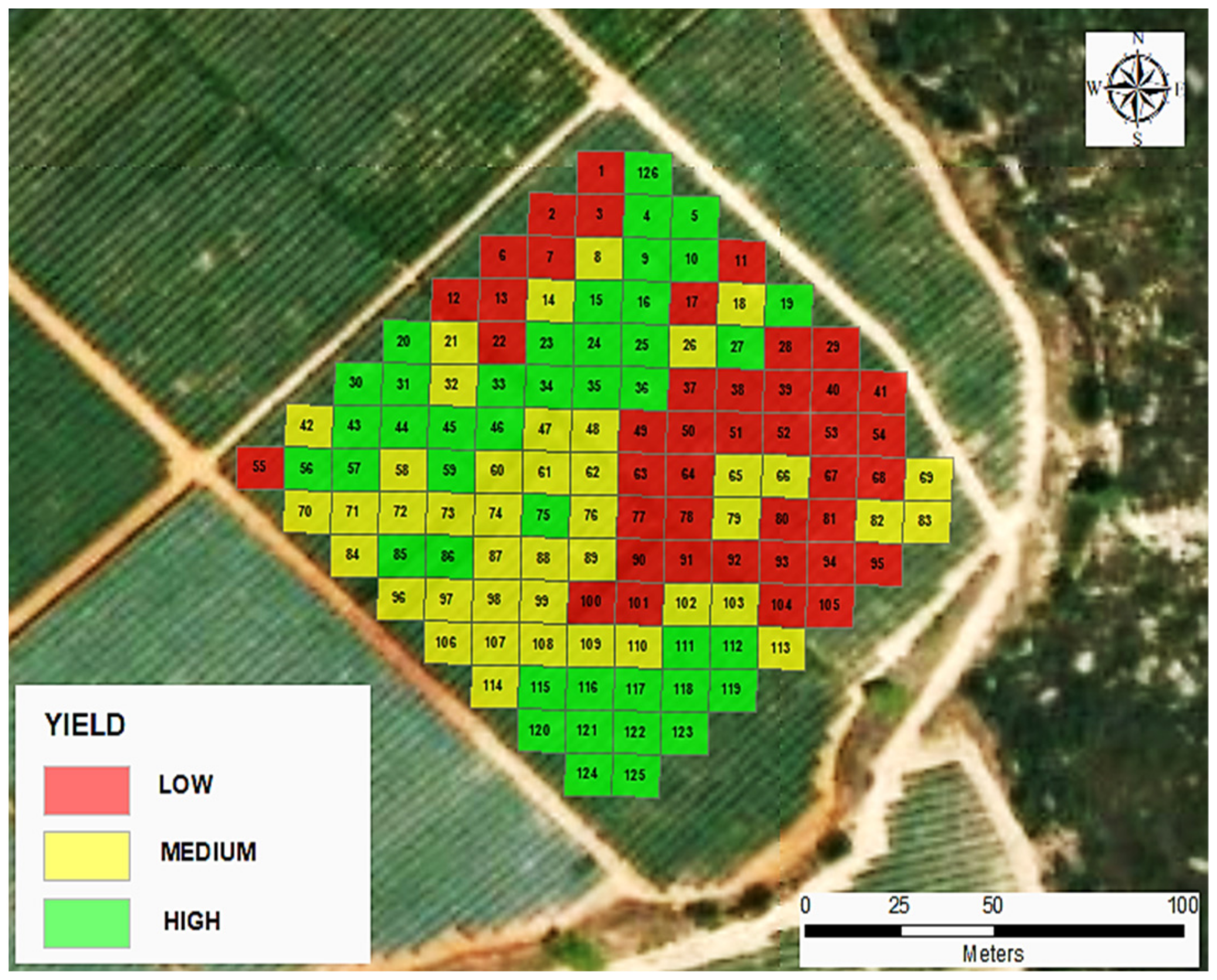
| Yield | 16.50 | 4.58 | 19.82 | 3.00 | 18.75 |
| Crop Circle ACS-470-NDVI | ||||||
|---|---|---|---|---|---|---|
| Sentinel-2 | GS | Correlation Coefficient Pearson-NDVI | Regression Model—NDVI | R-Squared (Adjusted for d.f.) (%) | MAE | p-Value |
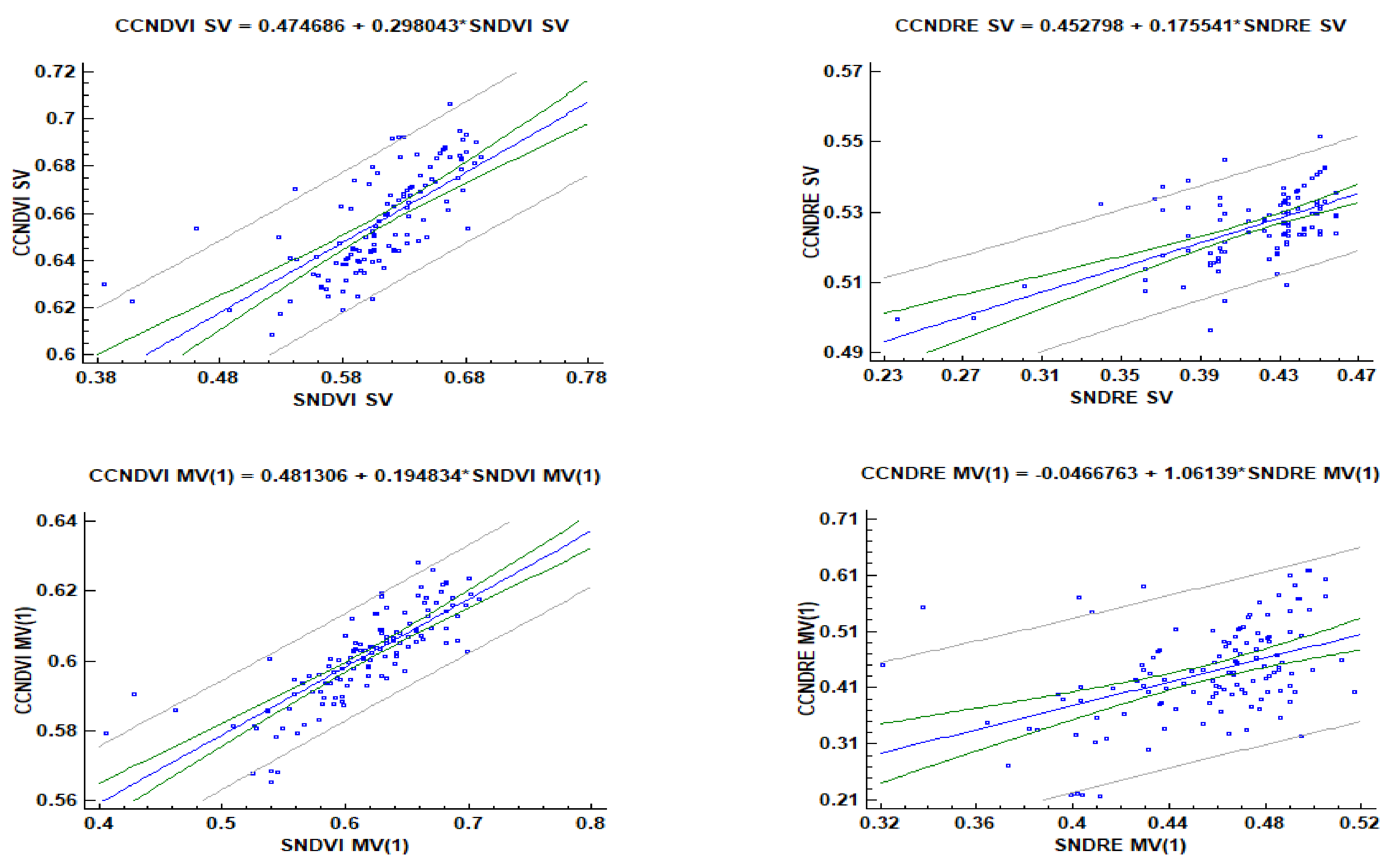
| SV | 0.71 | CCNDVI SV = 0.474686 + 0.298043 * SNDVI SV (5) | 50.39 | 0.0120 | 0.00 | |
| MV-1 | 0.80 | CCNDVI MV-1 = 0.481306 + 0.194834 * SNDVI MV-1 (6) | 64.36 | 0.0057 | 0.00 | |
| MV-2 | 0.70 | CCNDVI MV-2 = 0.524896 + 0.191779 * SNDVI MV-2 (7) | 48.85 | 0.0085 | 0.00 | |
| H-1 | 0.71 | CCNDVI H-1 = 0.571603 + 0.101303 * SNDVI H-1 (8) | 51.09 | 0.0051 | 0.00 | |
| H-2 | 0.79 | CCNDVI H(2) = 0.46648 + 0.192996*SNDVI H-2 (9) | 63.27 | 0.0085 | 0.00 | |
| Crop Circle ACS-470-NDRE | ||||||
| Sentinel-2 | GS | Correlation Coefficient Pearson-NDRE | Regression Model—NDRE | R-Squared (Adjusted for d.f.) | MAE | p-Value |
| SV | 0.60 | CCNDRE SV = 0.452798 + 0.175541 * SNDRE SV (10) | 35.50 | 0.0064 | 0.00 | |
| MV-1 | 0.45 | CCNDRE MV-1 = − 0.0466763 + 1.06139 * SNDRE MV-1 (11) | 19.58 | 0.0597 | 0.00 | |
| MV-2 | 0.55 | CCNDRE MV-2 = 0.252324 + 0.235186 * SNDRE MV-2 (12) | 29.35 | 0.0096 | 0.00 | |
| H-1 | 0.58 | CCNDRE H-1 = 0.204625 + 0.640423 * SNDRE H-1 (13) | 32.70 | 0.0370 | 0.00 | |
| H-2 | 0.37 | CCNDRE H-2 = 0.146509 + 0.573473 * SNDRE H-2 (14) | 13.16 | 0.0719 | 0.00 | |
| Growth Stages | Yield | |||
|---|---|---|---|---|
| CCNDVI | SNDVI | CCNDRE | SNDRE | |
| Pearson | ||||
| SV | 0.59 | 0.74 | 0.39 | 0.70 |
| MV-1 | 0.59 | 0.76 | 0.23 | 0.60 |
| MV-2 | 0.76 | 0.87 | 0.59 | 0.78 |
| H-1 | 0.50 | 0.65 | 0.30 | 0.60 |
| H-2 | 0.59 | 0.68 | 0.30 | 0.67 |
Publisher’s Note: MDPI stays neutral with regard to jurisdictional claims in published maps and institutional affiliations. |
© 2021 by the authors. Licensee MDPI, Basel, Switzerland. This article is an open access article distributed under the terms and conditions of the Creative Commons Attribution (CC BY) license (https://creativecommons.org/licenses/by/4.0/).
Share and Cite
Darra, N.; Psomiadis, E.; Kasimati, A.; Anastasiou, A.; Anastasiou, E.; Fountas, S. Remote and Proximal Sensing-Derived Spectral Indices and Biophysical Variables for Spatial Variation Determination in Vineyards. Agronomy 2021, 11, 741. https://doi.org/10.3390/agronomy11040741
Darra N, Psomiadis E, Kasimati A, Anastasiou A, Anastasiou E, Fountas S. Remote and Proximal Sensing-Derived Spectral Indices and Biophysical Variables for Spatial Variation Determination in Vineyards. Agronomy. 2021; 11(4):741. https://doi.org/10.3390/agronomy11040741
Chicago/Turabian StyleDarra, Nicoleta, Emmanouil Psomiadis, Aikaterini Kasimati, Achilleas Anastasiou, Evangelos Anastasiou, and Spyros Fountas. 2021. "Remote and Proximal Sensing-Derived Spectral Indices and Biophysical Variables for Spatial Variation Determination in Vineyards" Agronomy 11, no. 4: 741. https://doi.org/10.3390/agronomy11040741